Application of Response Surface Methodology for H2S Removal from Biogas by a Pilot Anoxic Biotrickling Filter


Department of Chemical Engineering and Food Technologies, Wine and Agrifood Research Institute (IVAGRO), Faculty of Sciences, University of Cádiz, 11510 Puerto Real (Cádiz), Spain
*
Authors to whom correspondence should be addressed.
ChemEngineering 2019, 3(3), 66; https://doi.org/10.3390/chemengineering3030066
Submission received: 13 May 2019
/
Revised: 4 July 2019
/
Accepted: 11 July 2019
/
Published: 13 July 2019
(This article belongs to the Special Issue Advances in Biogas Desulfurization)
Abstract
:In this study, a pilot biotrickling filter (BTF) was installed in a wastewater treatment plant to treat real biogas. The biogas flow rate was between 1 and 5 m3·h−1 with an H2S inlet load (IL) between 35.1 and 172.4 gS·m−3·h−1. The effects of the biogas flow rate, trickling liquid velocity (TLV) and nitrate concentration on the outlet H2S concentration and elimination capacity (EC) were studied using a full factorial design (33). Moreover, the results were adjusted using Ottengraf’s model. The most influential factors in the empirical model were the TLV and H2S IL, whereas the nitrate concentration had less influence. The statistical results showed high predictability and good correlation between models and the experimental results. The R-squared was 95.77% and 99.63% for the ‘C model’ and the ‘EC model’, respectively. The models allowed the maximum H2S IL (between 66.72 and 119.75 gS·m−3·h−1) to be determined for biogas use in a combustion engine (inlet H2S concentration between 72 and 359 ppmV). The ‘C model’ was more sensitive to TLV (–0.1579 (gS·m−3)/(m·h−1)) in the same way the ‘EC model’ was also more sensitive to TLV (4.3303 (gS·m−3)/(m·h−1)). The results were successfully fitted to Ottengraf’s model with a first-order kinetic limitation (R-squared above 0.92).
1. Introduction
Biogas, due to methane high combustion enthalpy, can be considered as an important renewable energy source. Nowadays, international laws such as the Directive of the European Parliament 2009/28/EC (April 23, 2009) recognize biogas as a source of vital energy that can reduce the European Union’s energy dependence. The aim of this directive is to increase consumption of renewable energy by 2020 by at least 20%. The longer-term goal is to achieve net-zero greenhouse emissions by 2050 and it will be necessary to increase investment in clean and energy-efficient technologies by 2.8% of Gross Domestic Product (GDP) (or around € 520–575 billion annually) [1]. Hydrogen sulfide (H2S) is one of the biggest pollutants in biogas. Therefore, it is necessary to reduce the generation of H2S in the digester and/or reduce its concentration for most uses of biogas. Apart from its harmful effects on health, the presence of H2S in biogas is not desirable because it is a corrosive gas. Desulfurization of biogas can be carried out by physical-chemical or biological processes. Physical-chemical processes have been commonly used but biological ones have proven to be a good competitor from economic and environmental points of view [2].
In biological processes the most widely used and studied microorganisms belong to the group of bacterial chemotrophic species, which use reduced sulfur compounds as an energy source and use oxygen (aerobic) or nitrate/nitrite (anoxic) as electron acceptors [3,4]. The biodesulfurization of biogas involves the use of technologies that facilitate appropriate contact between the gas and the liquid. There are several advantages in the use of anoxic biotrickling filters (BTFs) over aerobic ones, and these include reducing the risk of explosion, no dilution of biogas, and a lower limitation in the transfer of matter for nitrate when compared to the necessary oxygen absorption [5,6]. In contrast, the cost and availability of large amounts of nitrate can be limiting for the application of anoxic systems. Although ammonia-rich wastewater could be nitrified and used, Zeng et al. [3] used a biogas digestion slurry after nitrification to feed a BTF to achieve stable operation.
The H2S inlet load (IL) in BTFs is an important parameter in the design of this type of equipment. The IL and the elimination capacity (EC) describe the performance of the BTFs with respect to the removal efficiency (RE) of the contaminant and allow the design of the system, depending on the biogas flow rate that needs to be treated and the inlet H2S concentration. Values for a critical EC of between 100 and 130 gS·m−3·h−1 and a maximum EC between 140 and 280 gS·m−3·h−1 have been reported for both aerobic and anoxic biotrickling filters [5,7].
A model can be applied to relate input variables (pollutant inlet concentration, gas flow, electron acceptor concentration, etc.) and design variables (specific surface area of the support, equipment dimensioning, etc.) with the outputs (concentration of the pollutant at the outlet, production of biological reaction products, consumption of reagents, etc.). Empirical models (black box models) are characterized by a high predictive power, but their parameters lack physical significance [8]. They are based on statistically significant relationships between the input and output variables. Stationary-state models have been used to describe biofilters since the early 1980s [9,10,11]. Anoxic BTFs have been described by empirical [12,13] and dynamic [14,15] models. For instance, Soreanu et al. [13] proposed a second-order empirical model using a central composite design (CCD) and the biogas flow rate and the H2S concentration as input variables, with the H2S RE obtained as a response variable. Almenglo et al. [15] developed a model that considered the most relevant phenomena such as advection, absorption, diffusion and biodegration. Dynamic models provide a better understanding of the process, but their complexity means that they are seldom used for BTFs.
The aim of the work described here was to study the effects of gas (FG) and liquid (FL) flow rates and nitrate concentration ([N-NO3–]) along the packed bed on the outlet H2S concentration and the EC. Two empirical models were proposed to describe the outlet H2S concentration and the EC. Moreover, the H2S concentrations were measured along the bed and fitted using Ottengraf’s model [9].
2. Materials and Methods
2.1. Experimental Set-up
An anoxic BTF at pilot scale (Figure 1) was installed in the wastewater treatment plant (WWTP) ‘Bahía Gaditana’ (San Fernando, Spain) and it was fed with biogas from one of their sludge anaerobic digesters. The internal diameter was 0.5 m and the bed height was 0.85 m. The BTF was packed with open-pore polyurethane foam cubes (800 units, 25 kg·m−3, 600 m2·m−3) (Filtren TM25450, Recticel Iberica, Spain). The recirculation medium pH was kept at 7.4 and the temperature at 30 °C.
The nitrate feeding was done in batch mode and automatized by oxide reduction potential (ORP) (setpoint of −365 mV) [16]: when nitrate was exhausted a fixed liquid volume (25 L) was purged, then a nitrate solution (500 gNaNO3·L−1) was added to the recirculation medium and finally treated water from the WWTP was added to get a working volume. The nitrate depletion time (NDT) was the time between nitrate feedings, i.e., the time in which microorganisms consumed the nitrate added. NDT was dependent of IL and maximum nitrate concentration reached in the nitrate feeding cycle. The volume of the nitrate solution added was modified in concordance to maintain an NDT between 3 and 4 h. This volume ranged in a linear manner between 0.14 and 0.7 L for an H2S IL between 33.3 and 177 gS·m−3·h−1. During the nitrate depletion time the H2S concentrations in the outlet stream and along the bed height (0.2, 0.4, 0.6 and 0.8 m) were measured every 30 min, and samples of the recirculation medium were taken for nitrate, nitrite and sulfate measurement. Further information about the system can be found elsewhere [15,16]. A schematic representation of the experimental set-up is provided in Figure 2.
The H2S concentration in the biogas stream was measured using a gas chromatograph with a thermal conductivity detector (GC-450, Bruker, Germany) and a specific gas sensor (GAsBadge® Pro, Industrial Scientific, USA) was used for H2S concentrations below 500 ppmV. Sulfate, nitrite and nitrate were measured by a turbidimetric method (4-500-SO42− E), a colorimetric method (45000-NO2− B) and by an ultraviolet method (4500-NO3− B), respectively [17].
2.2. Experimental Design
A response surface model from a full factorial three-level three-factor design (33) was developed including two replicates at the central point. 33 design allows us to obtain a second-order polynomial using only three levels [18,19]. The three factors were gas flow rate (FG), liquid flow rate (FL) and nitrate concentration. The levels of the factor studied, and the values calculated for H2S IL (Equation (1)), trickling liquid velocity (TLV) (Equation (2)) and empty bed residence time (EBRT) (Equation (3)) are provided in Table 1.
where IL is the inlet load (gS·m−3·h−1), V is the bed volume (m3), [H2S]i is the inlet H2S concentration (gS·m−3), [H2S]o is the outlet H2S concentration (gS·m−3), RE is the removal efficiency, EC is the elimination capacity, TLV is the trickling liquid velocity (m·h−1), EBRT is the empty bed residence time (s) and A is the cross-sectional area of the bed (m2).
The experimental results were fitted with two empirical models. The first model, the concentration model (‘C model’), fitted the outlet H2S concentration as a response variable. The second model, the elimination capacity model (‘EC model’), fitted the EC as a response variable. In both models the independent variables were TLV, the H2S IL and the nitrate concentration (factors from Table 1). Instead of FG, H2S IL was chosen because the IL included the effect of the inlet H2S concentration (Equation (1)). In addition, TLV was used rather than FL because it allows a comparison with other BTFs. In both cases a second-order polynomial model was used to predict the outlet H2S concentration and the EC values. The data were analyzed using Statgraphics® Centurion XVIII (v.18.1.10).
2.3. Ottengraf’s Model
Ottengraf’s model [9,20] describes the concentration of pollutants in biofilters for steady-state processes. The analytical solution of the model was obtained in three ideal situations:
- There is no diffusion limitation and the biofilm is fully active, and hence the conversion rate is controlled by a zero-order reaction rate. The solution is described by Equation (6). K0 is a pseudo zero-order rate (g·m−3·s−1) and is proportional to the zero-order reaction rate constant (k0, Equation (7)).
- There is diffusion limitation and therefore the mass transfer rate to the biofilm is insufficient compared to biological substrate utilization rate. The solution is described by Equation (8).
- There is no diffusion limitation and the biofilm is fully active, and hence the conversion rate is controlled by a first-order reaction rate. The solution is described by Equation (6). K1 is a pseudo first-order rate constant (s−1) (Equation (10)) and is proportional to the first-order rate constant (k1, Equation (10)).
3. Results and Discussion
3.1. Empirical Model
The sulfate and nitrite concentrations were almost constant during the experiments; the sulfate concentration was 8.9 ± 1.6 gS-SO4·L−1 and nitrite concentration was between 0.1 and 10 mgN-NO2−·L−1. The H2S RE obtained during the experimentation carried out to obtain the empirical model is shown in Figure 3.
As expected, a high H2S RE was found at low FG (lower H2S IL). Therefore, the best results were for an FG of 1 m3·h−1, where the H2S IL was 35.1 ± 1.5 gS·m−3·h−1 and the RE between 97.3 and 99.5%. Under these conditions, the effects of the nitrate concentration and TLV were negligible. However, at higher biogas flow rates the decrease in the nitrate concentration led to a lower H2S RE. In anoxic biofiltration nitrate (or nitrite) is the electron acceptor, so its concentration must be a significant factor on the BTF performance, and this is even more important considering that the use of a nitrate feed controlled by ORP [16] leads to a decrease in the nitrate concentration until depletion.
The RE versus the TLV values for the three FG (EBRT of 600, 200 and 120 s) are listed in Table 2. When the nitrate concentration was not limiting, the TLV effect on H2S RE was only notable for an FG equal to or greater than 3 m3·h−1 (i.e. for H2S IL of 109.1 ± 11.7 and 172.4 ± 3.4 gS·m−3·h−1). Thus, for an FG of 3 m3·h−1, the H2S was between 84.7 and 97.6% and for 5 m3·h−1 the range was between 79.3 and 92.1%. The improvement observed could be explained by various effects: a higher wetted area [21], an increase in the hold-up liquid (6.4, 8.5 and 10.6 L for 5.1, 10.2 and 15.3 m·h−1) and a higher area in contact with the flowing liquid, as proposed by Almenglo et al. [15].
Consequently, the influence of the nitrate concentration in the recirculating liquid on the H2S RE was dependent of two factors: the H2S IL and the TLV. A higher TLV level supplies a higher nitrate availability in the biofilm. TLV has usually been kept constant in anoxic BTFs between 10 [22] and 15 [23] m·h−1, but for a high H2S IL it would be interesting to study the effect of this parameter. As in aerobic BTFs, where TLV is a key operational variable, in aerobic BTFs the regulation of TLV improves the oxygen mass transfer along the packed bed [24]. Fernández et al. [6] studied the effect of the TLV (2−20.5 m·h−1) on H2S RE in an anoxic BTF, for H2S ILs from 93 to 201 gS·m−3·h−1, packed with open pore polyurethane foam (the same support material as used in this study). It was found that there was no discernable influence for TLV values higher than 5 m·h−1 for H2S IL values below 157 gS·m−3·h−1. However, at an H2S IL of 201 gS·m−3·h−1 it was observed that TLV values below 15 m·h−1 produced a significant decrease in the H2S RE from 92 to 85% at 4.5 m·h−1. On using polypropylene Pall rings [25] the optimal TLV was also 15 m·h−1 at high H2S IL (>201 gS·m−3·h−1) although TLV did not have any effect at low H2S IL (< 78.4 gS·m−3·h−1). Zeng et al. [3] studied the effect of TLV between 2.63 an 9.47 m·h−1 (H2S IL < 86.92 gS·m−3·h−1) and achieved an efficient removal of H2S for the lowest TLV, probably due to the larger height-diameter (H/D) ratio (10.9) and the higher EBRT (342 s). A high H/D ratio and a low EBRT improve the gas-liquid mass transfer [26] but increase the installation cost due to the higher pressure drop [27] and the higher volume of the packed bed.
The statistical results for the ‘C model’ show the significance and high predictability of the regression model. The R-squared was 95.77%, the residual standard deviation was 0.1784 and the mean absolute error was 0.1224. The Durbin–Watson statistic was 1.00088 (p-value = 0.0001) and this shows a possible autocorrelation in the sample with a significance level of 5.0%. Moreover, the plot of residual versus predicted values (Figure 4a) does not show any patterns and we can assume a good correlation between the model prediction and the experimental results. The second-order polynomial model fitted with calibration data is represented by Equation (11).
As can be seen in Figure 4b, the most influential factor on the outlet H2S concentration was the H2S IL (p-value 2.26·10−8). Moreover, the TLV and nitrate concentration had a negative effect on the outlet H2S concentration with p-values of 5.26·10−14 and 5.34·10−4, respectively. It is interesting to note that the interaction AB (IL and TLV) was significant (p-value 1.18·10−5) and therefore the effect of one variable depended on the value of another. This behavior can be seen in Figure 3, where the TLV had an effect on the RE at high H2S IL but not at low ones.
The response surface for the ‘C model’ is shown in Figure 5. The model can be used to predict the factor limits to achieve a desired H2S outlet concentration. Depending on the combustion engine company, the inlet H2S limit is in the range 100–500 mg·Nm−3 (72–359 ppmV at 25 °C) [28]. Therefore, for a nitrate concentration of 35.5 mgN-NO3−·L−1 and TLV of 15.27 m h−1 the maximum H2S IL would be 66.72 and 119.75 gS·m−3·h−1 for outlet H2S concentrations of 72 and 359 ppmV, respectively.
The statistical results for the ‘EC model’ show a higher significance and predictability of the regression model when compared with the ‘C model’. The R-squared was 99.63%, the residual standard deviation was 2.545 and the mean absolute error was 1.646. The Durbin–Watson statistic was 1.7041 (p-value = 0.0626), although the p-value was higher than 5% there were no traces of autocorrelation—as verified by checking the residual plot (Figure 6a). The second-order polynomial model fitted with calibration data is represented by Equation (12).
As can be seen in Figure 6b, the most influential factor on the EC was the H2S IL (p-value 1.81·10−28). Moreover, the TLV and nitrate concentration had a positive effect on the EC with p-values of 2.37·10−11 and 1.38·10−5, respectively. In this case, the interactions AB (IL and TLV) and BC (IL and nitrate concentration) and the quadratic term (BB or IL2) were more significant than the nitrate concentration. Therefore, H2S IL and TLV had a greater effect on the EC than the nitrate concentration.
The response surface for the ‘EC model’ is shown in Figure 7. As expected, for high H2S IL (>109.1 ± 11.7 gS·m−3·h−1) or high biogas flow rate (FG > 3 m3·h−1) an increase in EC was observed when the nitrate concentration and TLV were increased.
A sensitivity analysis was performed by calculating the partial derivative in both models [29]. The maximum and minimum values for the variation of estimated variables corresponding to each factor are provided in Table 3. For the ‘C model’ the maximum negative effect corresponded to a TLV of –0.1579 (gS·m−3)/(m·h−1) and the maximum positive effect was for an H2S IL of 0.0177 (gS·m−3)/(gS·m−3·h−1). However for the ‘EC model’ the maximum effects were due to TLV values of –1.252 (gS·m−3)/(m·h−1) and 4.3303 (gS·m−3)/(m·h−1).
3.2. Ottengraf’s Model
The concentration profiles along the bed height were analyzed using Ottengraf’s model, without nitrate concentration limitations, for H2S IL values between 33 and 176 gS·m−3·h−1 and TLV values between 5.09 and 15.27 m·h−1. The linear adjustments are provided in Table 4 according to the following simplifications: controlled by zero-order diffusion, zero-order kinetic and first-order kinetic. The behavior of the concentration profile for 5.09 m·h−1 and 130 and 170 gS·m−3·h−1 could be explained using a zero-order simplification for diffusion or kinetic. However, for all other conditions the first-order kinetic simplification can be applied. The kinetic constant was in the range between 0.0025 and 0.0092 s−1.
To our knowledge, Ottengraf’s model has not be applied to biogas desulfurization, although studies on H2S removal from air have been modeled using Ottengraf’s model [30,31,32,33].
Jin et al. [32] found that the zero-order kinetic limitation described the outlet H2S concentration (TLV of 0.62 m·h−1 and a maximum H2S IL around 30 gS·m−3·h−1). Oyarzún et al. [30] applied zero-order diffusion equations for an inlet H2S concentration below Ks (Monod saturation constant) and zero-order kinetic equation and inlet concentration above Ks. The microbial kinetic of the biotrickling filter presented in this work can be described by a Haldane model [15], with an affinity constant for sulfide (Ks) of 8.4 gS·m−3 and a gas concentration in equilibrium of 1.28 gS·m−3. This concentration is considerably lower than the minimum inlet concentration employed in this work (5.55 gS·m−3). Therefore, the study was carried out at an inlet H2S concentration higher than Ks with a first-order kinetic as obtained by Oyarzún et al. [30].
4. Conclusions
The influence of the nitrate concentration was dependent on TLV and H2S IL, with its influence increasing for lower TLV and higher H2S IL. The empirical models obtained by the response surface methodology for the factorial design of three factors at three levels (33) were able to predict the outlet H2S concentration and the EC with a R-squared of 95.77% and 99.63% without autocorrelation. The most influential factors on the outlet H2S concentration and EC were the H2S IL and TLV, with the nitrate concentration being less significant. For biogas use in a CHP system the maximum H2S IL should be between 66.72 and 119.75 gS·m−3·h−1 (TLV of 15.27 m·h−1 and nitrate concentration of 35.5 mgN-NO3−·L−1). Moreover, Ottengraf’s model was applied successfully considering a first-order kinetic limitation simplification with an R-squared above 0.92.
Author Contributions
Research design, D.C. and M.R.; methodology, F.A. and M.R.; investigation, F.A.; writing—original draft preparation, F.A.; writing—review and editing, M.R.; supervision, D.C. and M.R.; funding acquisition, D.C. and M.R.
Funding
This research was funded by MINISTERIO DE ECONOMÍA Y COMPETITIVIDAD, grant number CTM2009-14338-C03-02 and the Research Result Transfer Office of the University of Cádiz, grant number PROTO-05-2010.
Acknowledgments
The authors wish to express sincere gratitude to the WWTP “UTE EDAR Bahía de Cádiz” for allowing us to install the biotrickling filter in their plant.
Conflicts of Interest
The authors declare no conflict of interest.
References
- European Commission. A Clean Planet for All a European Strategic Long-Term Vision for a Prosperous, Modern, Competitive and Climate Neutral Economy; COM (2018) 773 Final; European Commission: Brussels, Belgium, 2018; pp. 1–25.
- Cano, P.I.; Colón, J.; Ramírez, M.; Lafuente, J.; Gabriel, D.; Cantero, D. Life cycle assessment of different physical-chemical and biological technologies for biogas desulfurization in sewage treatment plants. J. Clean. Prod. 2018, 181, 663–674. [Google Scholar] [CrossRef]
- Zeng, Y.; Luo, Y.; Huan, C.; Shuai, Y.; Liu, Y.; Xu, L.; Ji, G.; Yan, Z. Anoxic biodesulfurization using biogas digestion slurry in biotrickling filters. J. Clean. Prod. 2019, 224, 88–99. [Google Scholar] [CrossRef]
- Valle, A.; Fernández, M.; Ramírez, M.; Rovira, R.; Gabriel, D.; Cantero, D. A comparative study of eubacterial communities by PCR-DGGE fingerprints in anoxic and aerobic biotrickling filters used for biogas desulfurization. Bioprocess Biosyst. Eng. 2018, 41, 1165–1175. [Google Scholar] [CrossRef] [PubMed]
- Montebello, A.M.; Fernández, M.; Almenglo, F.; Ramírez, M.; Cantero, D.; Baeza, M.; Gabriel, D. Simultaneous methylmercaptan and hydrogen sulfide removal in the desulfurization of biogas in aerobic and anoxic biotrickling filters. Chem. Eng. J. 2012, 200–202, 237–246. [Google Scholar] [CrossRef]
- Fernández, M.; Ramírez, M.; Gómez, J.; Cantero, D. Biogas biodesulfurization in an anoxic biotrickling filter packed with open-pore polyurethane foam. J. Hazard. Mater. 2014, 264, 529–535. [Google Scholar] [CrossRef] [PubMed]
- Fortuny, M.; Baeza, J.; Gamisans, X.; Casas, C.; Lafuente, J.; Deshusses, M.; Gabriel, D. Biological sweetening of energy gases mimics in biotrickling filters. Chemosphere 2008, 71, 10–17. [Google Scholar] [CrossRef]
- Wainwright, J.; Mulligan, M. Environmental Modelling: Finding Simplicity in Complexity, 2nd ed.; John Wiley & Sons, Inc.: Hoboken, NJ, USA, 2013; ISBN 978-0-470-74911-1. [Google Scholar]
- Ottengraf, S.; Rehm, H.; Reed, G. Exhaust gas purification. In Biotechnology—A Comprehensive Treatise; Verlag Chemie: Weinheum, Germany, 1986; Volume 8, pp. 426–452. [Google Scholar]
- Shareefdeen, Z.; Baltzis, B.; Oh, Y.; Bartha, R. Biofiltration of Methanol Vapor. Biotechnol. Bioeng. 1993, 41, 512–524. [Google Scholar] [CrossRef]
- Baltzis, B.; Wojdyla, S.; Zarook, S. Modeling biofiltration of VOC mixtures under steady-state conditions. J. Environ. Eng. 1997, 123, 599–605. [Google Scholar] [CrossRef]
- Soreanu, G. Insights into siloxane removal from biogas in biotrickling filters via process mapping-based analysis. Chemosphere 2016, 146, 539–546. [Google Scholar] [CrossRef]
- Soreanu, G.; Falletta, P.; Béland, M.; Edmonson, K.; Ventresca, B.; Seto, P. Empirical modelling and dual-performance optimisation of a hydrogen sulphide removal process for biogas treatment. Bioresour. Technol. 2010, 101, 9387–9390. [Google Scholar] [CrossRef]
- López, L.; Dorado, A.; Mora, M.; Gamisans, X.; Lafuente, J.; Gabriel, D. Modeling an aerobic biotrickling filter for biogas desulfurization through a multi-step oxidation mechanism. Chem. Eng. J. 2016, 294, 447–457. [Google Scholar] [CrossRef] [Green Version]
- Almenglo, F.; Ramírez, M.; Gómez, J.; Cantero, D.; Gamisans, X.; Dorado, A. Modeling and control strategies for anoxic biotrickling filtration in biogas purification. J. Chem. Technol. Biotechnol. 2016, 91, 1782–1793. [Google Scholar] [CrossRef]
- Almenglo, F.; Ramírez, M.; Gómez, J.; Cantero, D. Operational conditions for start-up and nitrate-feeding in an anoxic biotrickling filtration process at pilot scale. Chem. Eng. J. 2016, 285, 83–91. [Google Scholar] [CrossRef]
- Clesceri, L.S.; Greenberg, A.; Eaton, A. Standard Methods for the Examination of Water and Waste Water, 20th ed.; American Public Health Association, American Water Works Association, Water Environment Federation: Washington, DC, USA, 1999; ISBN 0875532357. [Google Scholar]
- Veljković, V.B.; Veličković, A.V.; Avramović, J.M.; Stamenković, O.S. Modeling of biodiesel production: Performance comparison of box–Behnken, face central composite or full factorial design. Chin. J. Chem. Eng. 2018. [Google Scholar] [CrossRef]
- Montgomery, D.C. Design and Analysis of Experiments, 5th ed.; John Wiley & Sons, Inc.: Hoboken, NJ, USA, 2001; p. 208. ISBN 0-471-31649-0. [Google Scholar]
- Ottengraf, S.; Oever, V.A. Kinetics of organic compound removal from waste gases with a biological filter. Biotechnol. Bioeng. 1983, 25, 3089–3102. [Google Scholar] [CrossRef] [PubMed] [Green Version]
- Onda, K.; Takeuchi, H.; Okumoto, Y. Mass transfer coefficients between gas and liquid phases in packed columns. J. Chem. Eng. Jpn. 1968, 1, 56–62. [Google Scholar] [CrossRef]
- López, L.R.; Brito, J.; Mora, M.; Almenglo, F.; Baeza, J.A.; Ramírez, M.; Lafuente, J.; Cantero, D.; Gabriel, D. Feedforward control application in aerobic and anoxic biotrickling filters for H2S removal from biogas. J. Chem. Technol. Biotechnol. 2018, 93, 2307–2315. [Google Scholar] [CrossRef]
- Brito, J.; Valle, A.; Almenglo, F.; Ramírez, M.; Cantero, D. Progressive change from nitrate to nitrite as the electron acceptor for the oxidation of H2S under feedback control in an anoxic biotrickling filter. Biochem. Eng. J. 2018, 139, 154–161. [Google Scholar] [CrossRef]
- López, L.R.; Bezerra, T.; Mora, M.; Lafuente, J.; Gabriel, D. Influence of trickling liquid velocity and flow pattern in the improvement of oxygen transport in aerobic biotrickling filters for biogas desulfurization. J. Chem. Technol. Biotechnol. 2016, 91, 1031–1039. [Google Scholar] [CrossRef]
- Fernández, M.; Ramírez, M.; Pérez, R.; Gómez, J.; Cantero, D. Hydrogen sulphide removal from biogas by an anoxic biotrickling filter packed with Pall rings. Chem. Eng. J. 2013, 225, 456–463. [Google Scholar] [CrossRef]
- Ordaz, A.; Figueroa-González, I.; San-Valero, P.; Gabaldón, C.; Quijano, G. Effect of the height-to-diameter ratio on the mass transfer and mixing performance of a biotrickling filter. J. Chem. Technol. Biotechnol. 2018, 93, 121–126. [Google Scholar] [CrossRef]
- Lebrero, R.; Gondim, A.; Pérez, R.; García-Encina, P.A.; Muñoz, R. Comparative assessment of a biofilter, a biotrickling filter and a hollow fiber membrane bioreactor for odor treatment in wastewater treatment plants. Water Res. 2014, 49, 339–350. [Google Scholar] [CrossRef] [PubMed]
- Ramírez, M.; Gómez, J.; Cantero, D.; Ramírez, M.; Gómez, J.; Cantero, D. Biogas: Sources, Purification and Uses. In Hydrogen and Other Technologies; Studium Press LLC: Houston, TX, USA, 2015; Volume 11, pp. 296–323. ISBN 978-1-626990-72-2. [Google Scholar]
- Koda, M.; Dogru, A.H.; Seinfeld, J.H. Sensitivity analysis of partial differential equations with application to reaction and diffusion processes. J. Comput. Phys. 1979, 30, 259–282. [Google Scholar] [CrossRef]
- Oyarzún, P.; Arancibia, F.; Canales, C.; Aroca, G.E. Biofiltration of high concentration of hydrogen sulphide using Thiobacillus thioparus. Process Biochem. 2003, 39, 165–170. [Google Scholar] [CrossRef]
- Jaber, M.; Couvert, A.; Amrane, A.; Rouxel, F.; Cloirec, P.; Dumont, E. Biofiltration of H2S in air—Experimental comparisons of original packing materials and modeling. Biochem. Eng. J. 2016, 112, 153–160. [Google Scholar] [CrossRef]
- Jin, Y.; Veiga, M.C.; Kennes, C. Effects of pH, CO2, and flow pattern on the autotrophic degradation of hydrogen sulfide in a biotrickling filter. Biotechnol. Bioeng. 2005, 92, 462–471. [Google Scholar] [CrossRef] [PubMed]
- Shareefdeen, Z.M.; Ahmed, W.; Aidan, A. Kinetics and Modeling of H2S Removal in a Novel Biofilter. Adv. Chem. Eng. Sci. 2011, 1, 72–76. [Google Scholar] [CrossRef]
Figure 1.
Photograph of the pilot scale anoxic biotrickling filter.

Figure 2.
Experimental set-up. GSP—Gas Sampling Port; LSP—Liquid Sampling Port. 1: Biotrickling filter; 2: biogas compressor; 3: rotameters (3.1: biogas and 3.2 liquid); 4: Cryostat Bath; 5: pumps (5.1 NaNO3; 5.2 NaOH; 5.3 recirculation pump).
Figure 2.
Experimental set-up. GSP—Gas Sampling Port; LSP—Liquid Sampling Port. 1: Biotrickling filter; 2: biogas compressor; 3: rotameters (3.1: biogas and 3.2 liquid); 4: Cryostat Bath; 5: pumps (5.1 NaNO3; 5.2 NaOH; 5.3 recirculation pump).
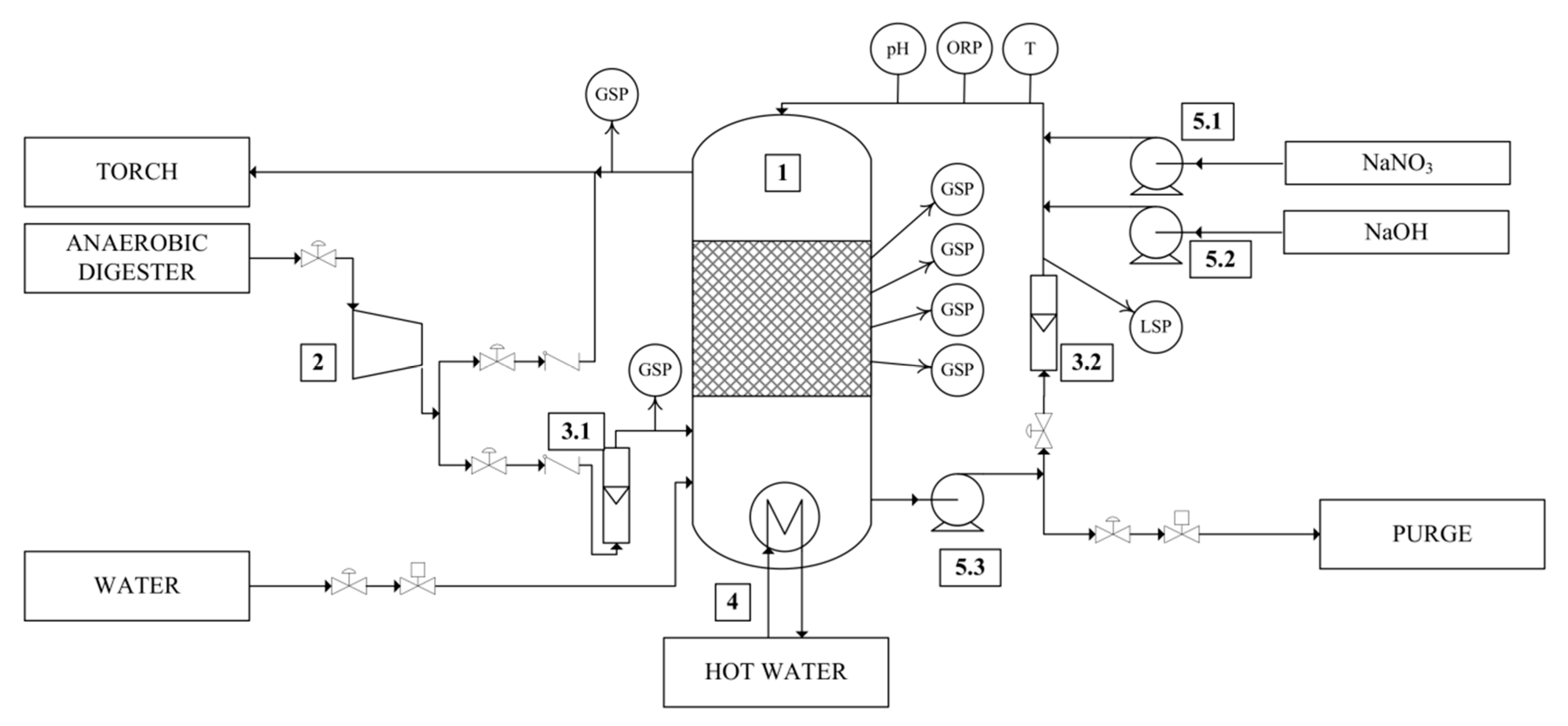
Figure 3.
Removal efficiency (RE) versus nitrate concentrations at different biogas (FG) and recirculation (FL) flow rates.
Figure 3.
Removal efficiency (RE) versus nitrate concentrations at different biogas (FG) and recirculation (FL) flow rates.
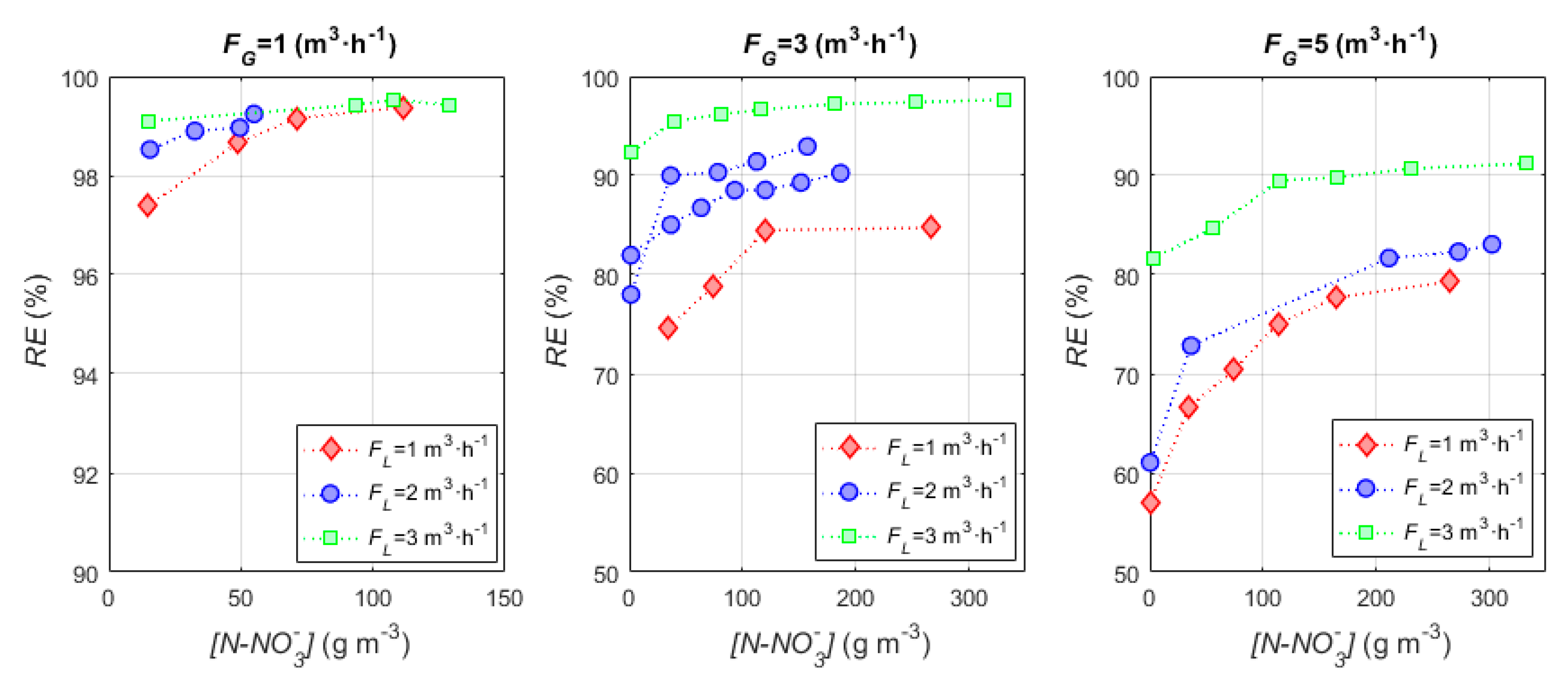
Figure 4.
Analysis for the ‘C model’: Residual versus predicted (a) and Pareto chart (b).
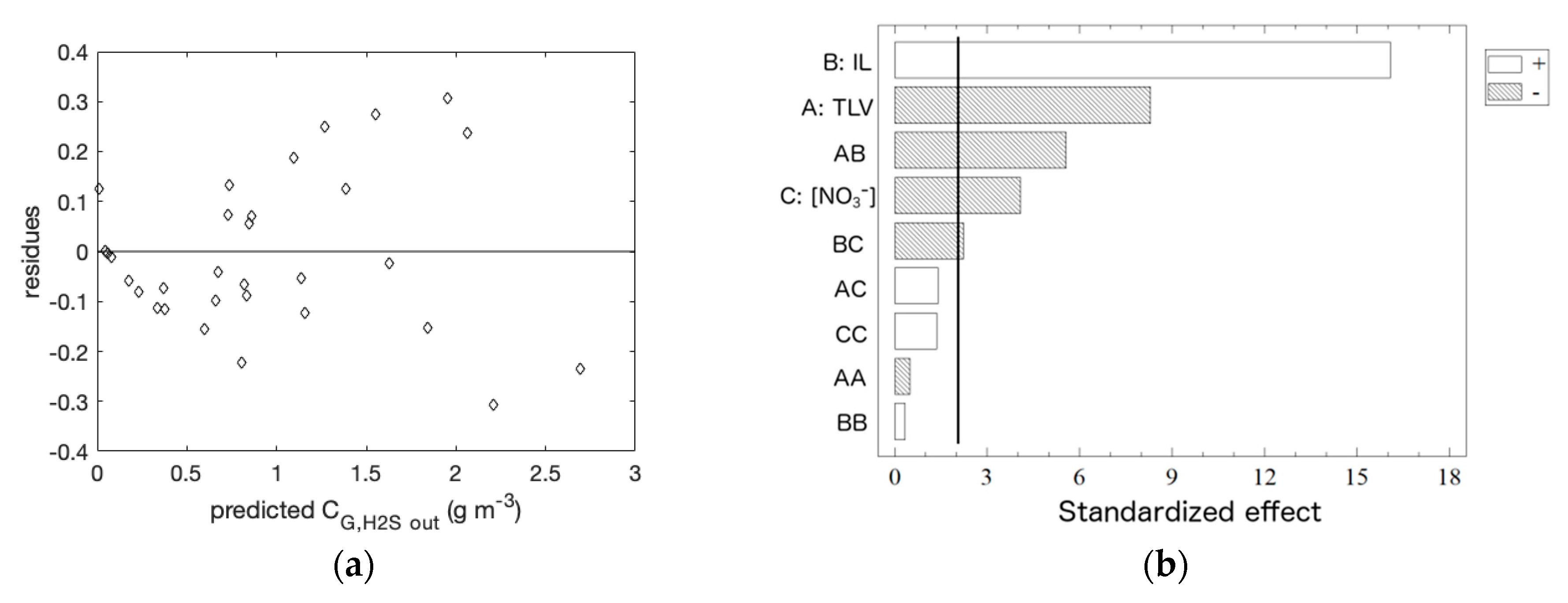
Figure 5.
Response surfaces for the ‘C model’.

Figure 6.
Analysis for the ‘elimination capacity (EC) model’: Residual versus predicted (a) and Pareto Chart (b).
Figure 6.
Analysis for the ‘elimination capacity (EC) model’: Residual versus predicted (a) and Pareto Chart (b).
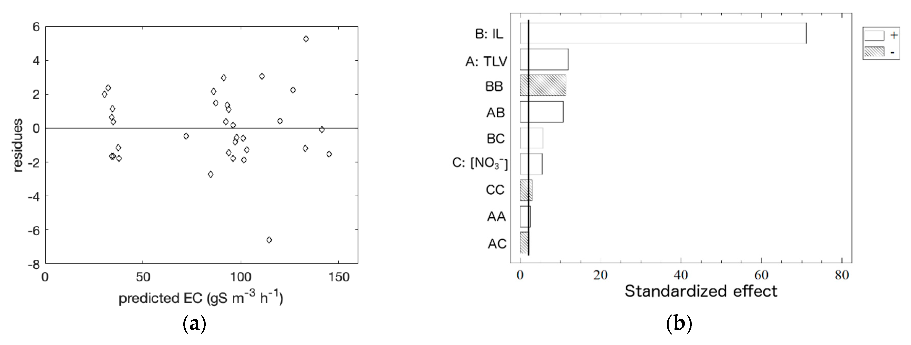
Figure 7.
Response surface for the ‘EC model’.


Table 1.
Levels of the factor tested in the experimental design (33).
| Factor | Levels of Factors | ||
|---|---|---|---|
| (–1) | (0) | (+1) | |
| FG (m3·h−1) | 1 | 3 | 5 |
| FL (m3·h−1) | 1 | 2 | 3 |
| [N-NO3−] (mg·L−1) | 1.4 ± 1.1 | 35.3 ± 2.4 | 70.5 ± 10.2 |
| IL1 (gS·m3·h−1) | 35.1 ± 1.5 | 109.1 ± 11.7 | 172.4 ± 3.4 |
| TLV2 (m·h−1) | 5.09 | 10.18 | 15.27 |
| EBRT1 (s) | 600 | 200 | 120 |
1 Values calculated for FG values of 1, 2, and 5 m3·h−1, respectively, 2 Values calculated for FL values of 1, 2 and 3 m3·h−1, respectively.
Table 2.
Removal efficiencies at different trickling liquid velocity (TLVs) and empty bed residence time (EBRT).
Table 2.
Removal efficiencies at different trickling liquid velocity (TLVs) and empty bed residence time (EBRT).
| TLV (m·h−1) | EBRT (s) 1 | ||
|---|---|---|---|
| 600 | 200 | 120 | |
| 5.09 | 99.39 | 84.73 | 79.31 |
| 10.18 | 99.24 | 93.08 | 83.06 |
| 15.27 | 99.53 | 97.65 | 92.13 |
1 The H2S ILs were 35.1±1.5, 109.1±11.7 and 172.4±3.4 gS·m−3·h−1, for 600, 200 and 120 s, respectively.
Table 3.
Sensitivity analysis.
| Factor | ‘C Model’ | ‘EC Model’ | ||
|---|---|---|---|---|
| Maximum | Minimum | Maximum | Minimum | |
| TLV | 0.0078 | –0.1579 | 4.3303 | –1.252 |
| IL | 0.0177 | 0.0045 | 1.1553 | 0.1657 |
| [N-NO3−] | 0.0038 | –0.159 | 0.4363 | –0.1801 |
Table 4.
Adjustments using Ottengraf’s model.
| IL (gS·m−3·h−1) | TLV (m·h−1) | Zero-Order Diffusion | Zero-Order Kinetic | First-Order Kinetic | |||
|---|---|---|---|---|---|---|---|
| r2 | k (s−1) | r2 | k (s−1) | r2 | k (s−1) | ||
| 36 | 5.09 | 0.62 | 0.0018 | 0.3 | 0.012 | 0.95 | 0.008 |
| 35 | 10.18 | 0.57 | 0.0018 | 0.26 | 0.012 | 0.92 | 0.0087 |
| 33 | 15.27 | 0.52 | 0.0018 | 0.22 | 0.011 | 0.93 | 0.0092 |
| 130 | 5.09 | 0.95 | 0.0011 | 0.94 | 0.011 | 0.93 | 0.0031 |
| 108 | 10.18 | 0.91 | 0.0012 | 0.82 | 0.01 | 0.93 | 0.0036 |
| 104 | 15.27 | 0.93 | 0.0014 | 0.77 | 0.01 | 0.96 | 0.0057 |
| 170 | 5.09 | 0.97 | 0.0009 | 0.96 | 0.0079 | 0.96 | 0.0025 |
| 176 | 10.18 | 0.88 | 0.001 | 0.79 | 0.0091 | 0.93 | 0.0029 |
| 167 | 15.27 | 0.86 | 0.0011 | 0.74 | 0.0092 | 0.95 | 0.0034 |
© 2019 by the authors. Licensee MDPI, Basel, Switzerland. This article is an open access article distributed under the terms and conditions of the Creative Commons Attribution (CC BY) license (http://creativecommons.org/licenses/by/4.0/).
Share and Cite
MDPI and ACS Style
Almenglo, F.; Ramírez, M.; Cantero, D. Application of Response Surface Methodology for H2S Removal from Biogas by a Pilot Anoxic Biotrickling Filter. ChemEngineering 2019, 3, 66. https://doi.org/10.3390/chemengineering3030066
AMA Style
Almenglo F, Ramírez M, Cantero D. Application of Response Surface Methodology for H2S Removal from Biogas by a Pilot Anoxic Biotrickling Filter. ChemEngineering. 2019; 3(3):66. https://doi.org/10.3390/chemengineering3030066
Chicago/Turabian StyleAlmenglo, Fernando, Martín Ramírez, and Domingo Cantero. 2019. "Application of Response Surface Methodology for H2S Removal from Biogas by a Pilot Anoxic Biotrickling Filter" ChemEngineering 3, no. 3: 66. https://doi.org/10.3390/chemengineering3030066