Circular Polarization near the Tight Focus of Linearly Polarized Light

Abstract

We have considered the tight focusing of light with linear polarization. Using the Richards–Wolf formalism, it is shown that before and after the focal plane, there are regions in which the polarization is circular (elliptical). When passing through the focal plane, the direction of rotation of the polarization vector is reversed. If before the focus in a certain area there was a left circular polarization, then directly in the focus in this area there will be a linear polarization, and after the focus in a similar area there will be a right circular polarization. This effect allows linearly polarized light to be used to rotate dielectric microparticles with little absorption around their center of mass.

1. Introduction

Sharp focusing of laser radiation is understood as the focusing of light by lenses with a high numerical aperture, and it is no longer possible to neglect the vector nature of the light wave. In this case, to calculate the light field at the focus, it is necessary to take into account all the components of the strength of the electric (or magnetic) field of the light wave. The classical formulas for calculating the light field in a sharp focus were obtained by Richards and Wolf in [1].

At present, a large number of works have been devoted to the sharp focusing of light. However, most of the works have been devoted to studying the behavior of the intensity at the focus, for example, obtaining focal spots of various shapes [2,3,4,5,6,7]. Much less work has been presented on the study of other characteristics of the light field, such as the energy flux (Poynting vector) [8,9,10], spin or orbital angular momentum [11,12,13,14]. We also note that the main attention of researchers has focused on the study of the behavior of light directly in focus; less attention has been paid to the behavior of light at some distance from the plane of sharp focus.

In this paper, the sharp focusing of linearly polarized light is considered. It is shown that, at a distance from the focal plane, regions arise in which the polarization ceases to be linear. In this case, when passing through the plane of focus, the direction of polarization in these regions changes to the opposite—in regions with right circular polarization, the direction changes to left circular and vice versa.

2. Theoretical background

In [1], expressions were obtained for the projections of the electric field strength vector at the focus of the aplanatic system. The Jones vector for an initial field with linear polarization directed along the y-axis has the form:

$$E_{lin}=A(\mathsf{\theta })\left(\begin{array}{l}0\\ 1\end{array}\right)$$

(1)

and the projections of the vector of the electric field strength and magnetic field strength near the focus for the initial field (1) have the form:

$$\begin{array}{l}{E}_x=-i{I}_{2,2}\sin 2\mathsf{\phi },\\ E_y=-i\left(I_{0,0}-I_{2,2}\cos 2\mathsf{\phi }\right),\\ E_z=-2I_{1,1}\sin \mathsf{\phi },\\ H_x=i\left(I_{0,0}+I_{2,2}\cos 2\mathsf{\phi }\right),\\ H_y=i{I}_{2,2}\sin 2\mathsf{\phi },\\ H_z=2I_{1,1}\cos \mathsf{\phi },\end{array}$$

(2)

where

$$I_{\nu ,\mu }=\left(\frac{\mathsf{\pi }f}{\mathsf{\lambda }}\right){\displaystyle \underset{0}{\overset{{\mathsf{\theta }}_0}{\int }}{\sin }^{\mathsf{\nu }+1}\left(\frac{\mathsf{\theta }}{2}\right){\cos }^{3-\mathsf{\nu }}\left(\frac{\mathsf{\theta }}{2}\right)}{\cos }^{1/2}(\mathsf{\theta })A(\mathsf{\theta })e^{ikz\cos \mathsf{\theta }}{J}_{\mathsf{\mu }}(x)d\mathsf{\theta },$$

(3)

where λ is the wavelength of light, f is the focal length of the aplanatic system, x = krsin θ, J_μ (x) is the Bessel function of the first kind, and NA = sin θ₀ is the numerical aperture. The angle φ in Equation (2) is the conventional polar (or azimuthal) angle in the transverse planes, including the focal plane. A positive angle value increases counterclockwise from the horizontal x-axis. In the initial plane, the light field has only linear polarization directed along the vertical y-axis, and the Jones vector (1) does not depend on the polar angle φ. In Equations (2) and (3), angle θ is the tilt angle of the rays to the optical axis, θ₀ is the maximal tilt angle, determining the numerical aperture NA, z is the direction of the optical axis, z = 0 is the focal plane, k is the wavenumber of light, (x, y) are the Cartesian coordinates in the cross-sections of the light beam converging into the focus (x is the horizontal axis, y is the vertical axis). The initial amplitude function A (θ) (suppose it is a real function) can be constant (plane wave) or in the form of a Gaussian beam. From (2), one can obtained the intensity distributions of each component of the electric vector.

$$\begin{array}{l}{I}_x=I_{2,2}^2{\sin }^2(2\phi ),\\ I_y=I_{0,0}^2+I_{2,2}^2{\cos }^2(2\phi )-2I_{0,0}{I}_{2,2}\cos (2\phi ),\\ I_z=4I_{1,1}^2{\sin }^2(\phi ).\end{array}$$

(4)

We note that Equations (1)–(4) differ from the equations obtained in [1], since the initial field (1) is polarized along the y-axis, whereas in [1] the initial field was polarized along the x-axis. Although the initial light field (1) has only one component E_y, Maxwell’s equations indicate that, upon light propagation, all three components of the E-field appear. If the light field propagates at a small angle to the optical axis, then the other two field components (E_x and E_z) are small and can be neglected. At tight focusing, the light propagates at large angles to the optical axis, so that all three components of the E-field (2) have a comparable value [15,16]. It can be seen from (4) that the intensity distribution I_x of the horizontal projection of the electric vector in the plane of focus has the form of four local maxima (light spots), the centers of which are located on a circle centered on the optical axis and lying on the rays emanating from the center at angles φ = π/4, 3π/4, 5π/4 and 7π/4.

The intensity distribution I_y has the form of an almost circular spot with a maximum on the optical axis $I_y=I_{0,0}^2$. The difference from the round shape of the spot arises from the fact that the distribution of intensity I_y along the vertical axis (φ = π/2) is greater ($I_y={\left(I_{0,0}+I_{2,2}\right)}^2$) than along the horizontal axis (φ = 0, $I_y={\left(I_{0,0}-I_{2,2}\right)}^2$). The intensity distribution (4) at the focus of the longitudinal component of the electric vector I_z has the form of two light spots, the centers of which lie on the vertical axis. This type of intensity distribution of electric vector individual components leads to the fact that the distribution of the total intensity at the focus has the form of an ellipse elongated along the vertical axis:

$$I=I_x+I_y+I_z=I_{0,0}^2+I_{2,2}^2+2I_{1,1}^2-2\left(I_{1,1}^2+I_{0,0}{I}_{2,2}\right)\cos (2\phi ).$$

(5)

Let us find the longitudinal component of the spin angular momentum (SAM) vector near the field focus (1) using the formula [17]:

$$S=\left(\frac{c^2{\epsilon }_0}{2\omega }\right)\mathrm{Im}\left(E*\times E\right)$$

(6)

where c is the speed of light in vacuum, ω is the angular frequency of the monochromatic light, ε₀ is the vacuum permittivity, Im is the imaginary part of the number, × is the sign of vector multiplication, * is the sign of complex conjugation. Below, we omit the constant $[(c^2{\epsilon }_0)/(2\omega )]$ for brevity. We note that sometimes, due to the electric–magnetic democracy, Equation (6) is written with two terms rather than one: $[c^2/(2\omega )] \mathrm{Im}\left[{\epsilon }_0\left(E*\times E\right)+{\mu }_0\left(H*\times H\right)\right]$, with μ₀ being the vacuum permeability (c²ε₀=µ₀⁻¹). However, immediately from the expression for the Poynting vector, only one term is obtained either for the E-vector or for the H-vector [17]. In addition, due to their different constants, both terms will give different contribution to the components of the SAM vector. Thus, Expression (6) is correct. Substituting from (2) into (6), we will assume that integrals (3) are complex, since z is different from zero. We get:

$$S_z=2\mathrm{Im}\left(E_x^{*}{E}_y\right)=2\sin (2\phi )\mathrm{Im}\left(I_{2,2}^{*}\left(I_{0,0}-\cos (2\phi )I_{2,2}\right)\right)$$

(7)

Certainly, near the tight focus, all 6 components of the E- and H-vectors (2) are significant, and none of these components can be neglected. Therefore, similarly to Equation (7), we can write expressions for the components S_x and S_y:

$$\begin{array}{l}{S}_x=2\mathrm{Im}\left(E_y^{*}{E}_z\right)=4\sin (\phi )\mathrm{Re}\left(I_{1,1}\left(\cos (2\phi )I_{2,2}^{*}-I_{0,0}^{*}\right)\right),\\ S_y=2\mathrm{Im}\left(E_z^{*}{E}_x\right)=4\sin (\phi )\sin (2\phi )\mathrm{Re}\left(I_{1,1}^{*}{I}_{2,2}\right).\end{array}$$

(8)

Let us single out the real and imaginary parts of the integrals included in (7) $I_{0,0}=R_0+i{I}_0, I_{2,2}=R_2+i{I}_2$. Then, instead of (7), we write:

$$S_z=2\sin (2\phi )\left(I_0{R}_2-I_2{R}_0\right)$$

(9)

The integrals R₀, R₂ in (9) include the comultiplier cos (kzcosθ) ≈ 1 at kz << 1, and the integrals $I_0 ,I_2$ include the comultiplier $\sin \left(kz\cos \theta \right)\approx kz\sin \theta$ at kz << 1. With this in mind, instead of (9), we write:

$$S_z\approx 2kz\sin (2\phi )\left({\overline{I}}_0{\overline{R}}_2-{\overline{I}}_2{\overline{R}}_0\right)$$

(10)

In (10), the following notations are used:

$$\begin{array}{l}{\overline{R}}_0=I_{0,0}(z=0), {\overline{R}}_2=I_{2,2}(z=0),\\ {\overline{I}}_0={\overline{I}}_{0,0}(z=0), {\overline{I}}_2={\overline{I}}_{2,2}(z=0),\\ {\overline{I}}_{\nu ,\mu }=\left(\frac{\pi f}{\lambda }\right){\displaystyle \underset{0}{\overset{{\theta }_0}{\int }}{\sin }^{\nu +1}\left(\frac{\theta }{2}\right){\cos }^{3-\nu }\left(\frac{\theta }{2}\right)}{\cos }^{3/2}(\theta )A(\theta )e^{ikz\cos \theta }{J}_{\mu }(x)d\theta .\end{array}$$

(11)

Let, on a circle of some radius, the expression in parentheses in (10) be greater than zero ${\overline{I}}_0{\overline{R}}_2-{\overline{I}}_2{\overline{R}}_0>0$, and since sin (2φ) in (10) is positive in quadrants 1 and 3, and negative in 2 and 4, then before the focus (z < 0) the longitudinal component SAM S_z in (10) will be positive in quadrants 2 and 4, and negative in 1 and 3. Moreover, since the sign of the entire expression after the focus (z > 0) changes to the opposite, the longitudinal component of SAM S_z in (9) is positive in quadrants 1 and 3, and negative in 2 and 4. This means that before the focus in the quadrants 2 and 4, the polarization vector rotates counterclockwise (right circular or elliptical polarization), and after the focus in these quadrants, the polarization vector rotates clockwise (left circular or elliptical polarization). Recall that in the plane of focus, the light at each point only has linear polarization, since at z = 0 the longitudinal component of the SAM S_z in (10) is equal to zero. The defocusing magnitude z in Equation (10) affects the size of the areas in the transverse plane, where polarization is not linear. At a distance z nearly equal to λ, the size of the circular polarization area is maximal (for NA = 0.95 it is approximately λ/2). As z tends to zero (i.e., in the focus), the size of the area with circular polarization decreases to zero.

Note also that the longitudinal component of the SAM is exactly equal to the third component of the Stokes vector:

$$S_z=2\mathrm{Im}\left(E_x^{*}{E}_y\right)=s_3,$$

(12)

which shows the presence of circular and elliptical polarization in the light field. In the next section, the presented theoretical predictions will be confirmed by simulation.

We note that the change in the rotation direction of the polarization vector to the opposite beyond the focal plane, as follows from Equation (10), can be explained by the angular momentum (AM) conservation law. Since polarization in the initial plane and in the focal plane is locally linear, S_z = 0. Therefore, if there are areas with left-handed circular polarization before the focus, then beyond the focus, circular polarization in these areas should become right-handed. However, the presence of such areas near the focus does not follow from the AM conservation.

3. Simulation by Richards–Wolf Formula

In this work, using the Richards–Wolf formulas, the focusing of a linearly polarized plane wave (wavelength 633 nm) was simulated by choosing a lens with NA = 0.95. The field near the tight focus was calculated using the integrals [1]:

$$\begin{array}{l}U\left(\mathsf{\rho },\mathsf{\psi },\mathrm{z}\right)=-\frac{if}{\mathsf{\lambda }}{\displaystyle \underset{0}{\overset{{\mathsf{\theta }}_0}{\int }}{\displaystyle \underset{0}{\overset{2\mathsf{\pi }}{\int }}B\left(\mathsf{\theta },\mathsf{\phi }\right)T\left(\mathsf{\theta }\right)P\left(\mathsf{\theta },\mathsf{\phi }\right)\times }}\\ \times \exp \left\{ik\left[\mathsf{\rho }\sin \mathsf{\theta }\cos \left(\mathsf{\phi }-\mathsf{\psi }\right)+z\cos \mathsf{\theta }\right]\right\}\sin \mathsf{\theta } \mathrm{d}\mathsf{\theta } \mathrm{d}\mathsf{\phi },\end{array}$$

(13)

where U (ρ, ψ, z) is the strength of the electric or magnetic field, B (θ, φ) is the electric or magnetic field at the input of the wide-aperture system in coordinates of the exit pupil (θ is the polar angle, φ is the azimuthal angle), T (θ) is the lens apodization function, f is the focal length, k = 2π/λ is the wavenumber, λ is the wavelength (in the simulation it was considered equal to 633 nm) and α_max is the maximum polar angle determined by the numerical aperture of the lens (NA = sin θ₀); P (θ, φ) is the polarization vector, for the strength of the electric and magnetic fields has the form:

$$P\left(\mathsf{\theta },\mathsf{\phi }\right)=\left[\begin{array}{c}1+{\cos }^2\mathsf{\phi }\left(\cos \mathsf{\theta }-1\right)\\ \sin \mathsf{\phi }\cos \mathsf{\phi }\left(\cos \mathsf{\theta }-1\right)\\ -\sin \mathsf{\theta }\cos \mathsf{\phi }\end{array}\right]a\left(\mathsf{\theta },\mathsf{\phi }\right)+\left[\begin{array}{l}\sin \mathsf{\phi }\cos \mathsf{\phi }\left(\cos \mathsf{\theta }-1\right)\\ 1+{\sin }^2\mathsf{\phi }\left(\cos \mathsf{\theta }-1\right)\\ -\sin \mathsf{\theta }\sin \mathsf{\phi }\end{array}\right]b\left(\mathsf{\theta },\mathsf{\phi }\right),$$

(14)

where a (θ, φ) and b (θ, j) are functions describing the polarization state of the x- and y-components intensities of the focused beam. In contrast to Equations (2) and (3), we gave Equations (13) and (14) in a general form to show that further modeling is carried out by the general Equations (13) and (14) and that the simulation results confirm the theoretical conclusions, following from Equations (11) and (12). After calculating the components of the electric field, the behavior of the components of the Stokes vector near the sharp focus were determined. The Stokes vector components were calculated using the formulas:

$$\begin{array}{l}{s}_0=E_x{E}_x^{*}+E_y{E}_y^{*},\\ s_1=E_x{E}_x^{*}-E_y{E}_y^{*},\\ s_2=2\mathrm{Re}\left(E_x^{*}{E}_y\right),\\ s_3=2\mathrm{Im}\left(E_x^{*}{E}_y\right).\end{array}$$

(15)

Similarly to Equations (7)–(9), the substitution of Equation (2) into Equation (15) allows us to obtain explicit expressions for the Stokes components s₁ and s₂ near the focus. For instance, a simpler expression is derived for s₂ at kz << 1:

$$s_2\approx 2\sin (2\phi ){\overline{R}}_2\left({\overline{R}}_0-{\overline{R}}_2\cos (2\phi )\right)$$

(16)

At small kz << 1, the second Stokes component (16) does not depend on z and therefore does not change sign when passing through the focus (z = 0). Below, this is confirmed by simulation. Similarly, the first Stokes component s₁ in Equation (15), expressed via the components of the E-vector (2), is also independent of z near the focus.

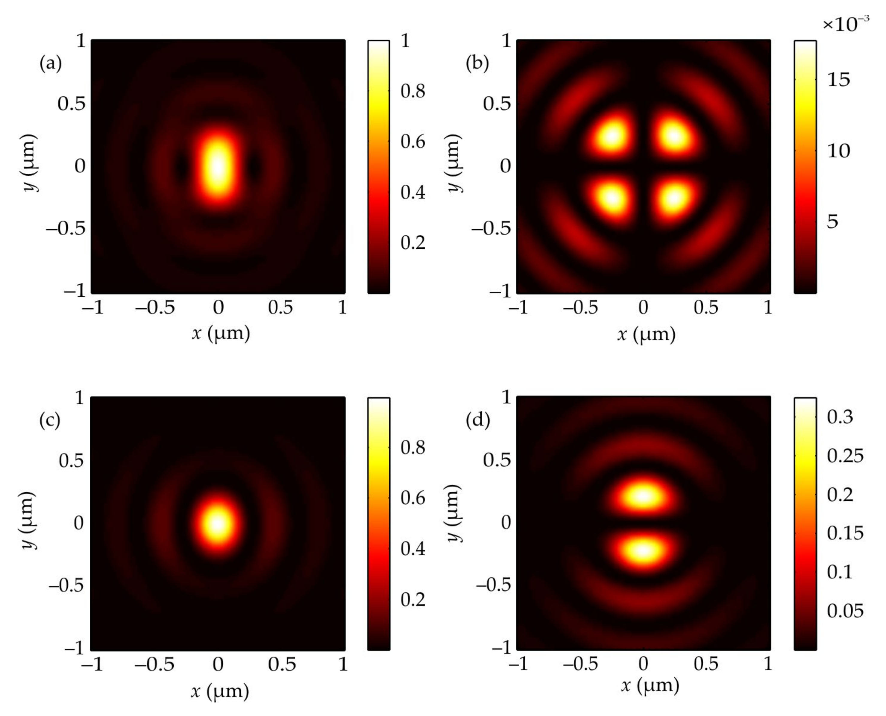
To estimate the relative contribution of individual polarization components, it is convenient to use the Stokes vector components normalized to the transverse intensity: $\left(S_1,S_2,S_3\right)=\left(s_1/s_0,s_2/s_0,s_3/s_0\right)$. It is known that when focusing light of linear polarization at the focus, all three components of the electric field strength are observed [18]. Figure 1 illustrates the distribution of the total intensity and its individual components in the focus of an aplanatic lens with NA = 0.95, when focusing a plane wave with a wavelength of 633 nm and polarization along the y-axis. To estimate the effect of defocusing, Figure 2 shows the same distributions of the total intensity and of the individual intensity components as in Figure 1, but at a distance λ from the focal plane. The intensity distributions have the same shape at the same distance before and after the focus.

Figure 1 shows that the initial component makes the main contribution to the focal spot formation, but the longitudinal component of the intensity also begins to make a significant contribution. The component perpendicular to the input polarization is rather small but present, while the light at the focus is still linearly polarized. Note that the distributions of the total intensity at the focus and the intensity of individual components in Figure 1 confirm the theoretical predictions that follow from Equations (4) and (5). Figure 2 indicates that a small shift from the focal plane (by a distance λ) leads to a decrease of the maximum intensity five times.

The distribution of the components of the Stokes vector (s₁, s₂, s₃) and the normalized components of the Stokes vector (S₁, S₂, S₃) at the distance z = λ after the focus is shown in Figure 3 and Figure 4, respectively.

From Figure 3 and Figure 4, it can be seen that the polarization after focus is predominantly linear. In the center of the focal spot in Figure 3a, a minimum is observed, which indicates that the polarization at the focus is directed along the y axis. This is also confirmed by Figure 4a: for a wave fully polarized along the y-axis S₁ = −1. From Figure 4a, it can be seen that the polarization does not change its direction at the focus and along the x and y axes, but along the straight lines located at an angle of ± 45° to the axes, the deviation from the initial polarization turns out to be maximum. From Figure 3 and Figure 4, it is also seen that the diverging beam contains regions with circular polarization. Recall that there are no such regions at the focus itself—the light is linearly polarized. From Figure 4c it is seen that the contribution of the circular polarization in such regions is quite noticeable—for S₃ = ±1, the polarization is completely circular, but there, in some regions, S₃ reaches values of ±0.8.

Figure 5 and Figure 6 similarly show the distribution of the Stokes vector and normalized Stokes vector at a distance of one wavelength in front of the focus.

A comparison of Figure 4, Figure 5 and Figure 6 shows that the first two components of the Stokes vector describing the linear polarization have not changed, and the third has changed its sign to the opposite. After passing the plane of the focus, the direction of the circular (elliptical) polarization is reversed—for example, in the first quadrant, the light in front of the focus plane had a left circular polarization, and after focus, a right polarization. Before the focus, the right circular (elliptical) polarization appears in the second and fourth quadrants and the left circular polarization appears in the first and third quadrants (Figure 6c). It agrees with the theoretical prediction based on Expression (10), and the change in the direction of rotation of the polarization vector in these quadrants after passing through the focus also follows from (10).

Below, we show how the distribution of S₃ changes with the distance from the focal plane. Figure 7 shows the intensity distribution (Figure 7a) and the longitudinal Stokes component S₃ (Figure 7b) in the longitudinal plane yz along the z-axis, rotated by an angle ϕ = 45° (i.e., passing through the S₃ maximum in Figure 6).

Figure 7 demonstrates that in the focal plane, the light field is linearly polarized. However, directly beyond the focal plane, areas with an elliptical polarization are generated (red areas in Figure 7). It is also interesting that as we move away from the focus, the direction of rotation of the polarization vectors changes to the opposite (blue areas in Figure 7). Figure 7b also shows how the size of the area with elliptical polarization changes with the distance z.

4. Modeling the Formation of Circular Polarization Using the FDTD Method

To check the correctness of the calculations by the Richards–Wolf formulas, an additional simulation was performed using the FDTD method. The focusing of a linearly polarized plane wave (λ = 633 nm) by a Fresnel zone plate with a focal length of f = 500 nm and a diameter of 7.9 μm was considered. The numerical aperture of such a lens is NA = 0.99. The focusing was simulated using the FDTD method implemented in FullWave software. Note that the FDTD method implemented in FullWave makes it possible to calculate the values of the electromagnetic field components at individual moments of time. To calculate the complex amplitude on the basis of individual instantaneous values of the field amplitudes, the method proposed in [19] was used. Figure 8 shows the distribution of the components of the normalized Stokes vector at a distance of one wavelength after the focus.

From Figure 8, it can be seen that simulating using the FDTD method confirms the results obtained using the Richards–Wolf formulas. In particular, Figure 8a shows that light is predominantly linearly polarized along the y-axis, and Figure 8c shows that quadrants 1 and 3 contain a right-handed circular polarization, and quadrants 2 and 4 a left-handed circular polarization.

Comparison of Figure 4 and Figure 8 indicates that although the structures of both patterns are similar, there are also significant differences. This is because the simulations by the Richards–Wolf method [1] and by the FDTD method [19] were carried out under different conditions. In the latter case, the tight focusing of light was simulated by passing the light field through a real Fresnel zone plate with a focal length equal to the wavelength (f = λ) and with a numerical aperture NA = 0.99. At the same time, the Richards–Wolf formalism adequately describes the light field at the focus of an ideal spherical lens if f >> λ. Thus, the Richards–Wolf formalism approximately describes the behavior of light near the focus, whereas the FDTD method, based on a rigorous solution of the Maxwell equations, adequately describes the behavior of light at the focus near the surface of the focusing zone plate. Therefore, modeling by the FDTD method expands the boundaries of the discovered optical phenomenon: a generation of local areas with circular (elliptical) polarization near the tight focus of light with initially linear polarization.

5. Reducing the Contribution of Circular Polarization with Decreasing Numerical Aperture of the Lens

Let us now consider the contribution of reducing the numerical aperture of the lens to NA = 0.6 (corresponding to a standard 40× aplanatic lens). The result is shown in Figure 9. Figure 9 shows that the maximum S₃ has decreased by two times. Moreover, from Figure 9a, it can be seen that the relative contribution of the linear polarization (along the y axis) increased significantly: the maximum in Figure 4 was equal to −0.5, and in Figure 9a to −0.92. Recall that for S₁ = ±1, the polarization is completely linear.

6. Calculation of the Moment of Forces Acting on a Dielectric Microparticle near the Focus

Let us calculate a force and a torque, acting onto a microbead from the light field. The force F and the torque M relative to an arbitrary point A, are equal to [20,21].

$$F=-{\displaystyle \underset{S}{\oint }\left(\sigma ·n\right)dS}$$

(17)

$$M={\displaystyle \underset{S}{\oint }\left[r\times \left(\sigma ·n\right)\right]dS}$$

(18)

where r is the radius-vector from the point A (x,y,z) to the point of integration on the surface S, n is an external normal vector to the surface S, A is the point relative to which the torque M is calculated and $\sigma$ is the Maxwell stress tensor, the components of which in the CGS system can be written as [22]

$${\sigma }_{ik}=\frac{1}{4\pi }\left(\frac{{\left|E\right|}^2+{\left|H\right|}^2}{2}{\delta }_{ik}-E_i{E}_k-H_i{H}_k\right)$$

(19)

where $E_i, H_i$ are the electric and magnetic field components and ${\delta }_{ik}$ is the Kronecker symbol (${\delta }_{i=k}=1$, ${\delta }_{i\ne k}=0$).

Shown in Figure 10 is a simulation result of the torque and force calculation acting on the spherical microbead.

Calculations show, that for the position of the particle X_p = 0.3 μm, Y_p = 0.3 μm the force projections are F_x = 2.79 pN, F_y = 3.7 pN and F_z = 8.78 pN. The torque projections are M_x = $2.81·{10}^{-19}$ Nm, M_y = $-5.55·{10}^{-19}$ Nm and M_z = $1.73·{10}^{-19}$ Nm. If we shift the bead at the position Xp = 0.3 μm, Y_p = −0.3 μm, then the result force projections become F_x = 2.66 pN, F_y = –3.58 pN and Fz = 8.9 pN, and the torque projections become M_x = $-3.0·{10}^{-19}$ Nm, M_y = $-5.9·{10}^{-19}$ Nm and M_z = $-1.5·{10}^{-19}$ Nm. Figure 10 shows that in the first quadrant, the axial torque is positive (M_z = $1.73·{10}^{-19}$ Nm), and in the fourth quadrant the torque is negative (M_z = $-1.5·{10}^{-19}$ Nm). This proves that the longitudinal projection of the CAM is positive in the first quadrant and negative in the fourth (Figure 8 and Figure 9).

7. Conclusions

In this work, theoretically, using the Richards–Wolf formalism and using two different modeling methods, it was shown that with the sharp focusing of light with a linear polarization in the planes before and after the focus, there were regions that arose in pairs in even and odd quadrants, and in these regions, light was circularly or elliptically polarized (for example, even to the right and odd to the left). Moreover, after passing through the focus in these areas, the direction of rotation of the polarization vector changes to the opposite (in even quadrants, it becomes left-handed, and in odd quadrants, it becomes right-handed circular or elliptical polarization). This result allows the use of linearly polarized light to rotate microparticles (the size of the circularly polarized region is about 0.3 μm by 0.3 μm) around its center of mass.

We note that a similar result has been obtained in [23]. It has been shown that certain structures allow the generation before the focus and beyond the focus of two conjugate optical vortices with opposite-sign topological charges and with longitudinal axial polarization. In our work, we have not used any additional structures.

References

- Richards, B.; Wolf, E. Electromagnetic diffraction in optical systems, II. Structure of the image field in an aplanatic system. Proc. R. Soc. Lond. Ser. A Math. Phys. Sci. 1959, 253, 358–379. [Google Scholar] [CrossRef]
- Yuan, G.H.; Wei, S.B.; Yuan, X.-C. Nondiffracting transversally polarized beam. Opt. Lett. 2011, 36, 3479–3481. [Google Scholar] [CrossRef] [PubMed]
- Ping, C.; Liang, C.; Wang, F.; Cai, Y. Radially polarized multi-Gaussian Schell-model beam and its tight focusing properties. Opt. Express 2017, 25, 32475–32490. [Google Scholar] [CrossRef]
- Grosjean, T.; Gauthier, I. Longitudinally polarized electric and magnetic optical nano-needles of ultra high lengths. Opt. Commun. 2013, 294, 333–337. [Google Scholar] [CrossRef]
- Wang, H.; Shi, L.; Lukyanchuk, B.; Sheppard, C.; Chong, C.T. Creation of a needle of longitudinally polarized light in vacuum using binary optics. Nat. Photon 2008, 2, 501–505. [Google Scholar] [CrossRef]
- Lin, J.; Chen, R.; Jin, P.; Cada, M.; Ma, Y. Generation of longitudinally polarized optical chain by 4π focusing system. Opt. Commun. 2015, 340, 69–73. [Google Scholar] [CrossRef]
- Zhuang, J.; Zhang, L.; Deng, D. Tight-focusing properties of linearly polarized circular Airy Gaussian vortex beam. Opt. Lett. 2020, 45, 296–299. [Google Scholar] [CrossRef]
- Lyu, Y.; Man, Z.; Zhao, R.; Meng, P.; Zhang, W.; Ge, X.; Fu, S. Hybrid polarization induced transverse energy flow. Opt. Commun. 2020, 485, 126704. [Google Scholar] [CrossRef]
- Li, H.; Wang, C.; Tang, M.; Li, X. Controlled negative energy flow in the focus of a radial polarized optical beam. Opt. Express 2020, 28, 18607. [Google Scholar] [CrossRef]
- Kotlyar, V.V.; Stafeev, S.S.; Nalimov, A.G. Energy backflow in the focus of a light beam with phase or polarization singularity. Phys. Rev. A 2019, 99, 033840. [Google Scholar] [CrossRef]
- Bomzon, Z.; Gu, M.; Shamir, J. Angular momentum and geometrical phases in tight-focused circularly polarized plane waves. Appl. Phys. Lett. 2006, 89, 241104. [Google Scholar] [CrossRef]
- Aiello, A.; Banzer, P.; Neugebauer, M.; Leuchs, G. From transverse angular momentum to photonic wheels. Nat. Photon. 2015, 9, 789–795. [Google Scholar] [CrossRef]
- Li, M.; Cai, Y.; Yan, S.; Liang, Y.; Zhang, P.; Yao, B. Orbit-induced localized spin angular momentum in strong focusing of optical vectorial vortex beams. Phys. Rev. A 2018, 97, 053842. [Google Scholar] [CrossRef]
- Zhao, Y.; Edgar, J.S.; Jeffries, G.; McGloin, D.; Chiu, D.T. Spin-to-Orbital Angular Momentum Conversion in a Strongly Focused Optical Beam. Phys. Rev. Lett. 2007, 99, 073901. [Google Scholar] [CrossRef] [PubMed]
- Monteiro, P.B.; Neto, P.A.M.; Nussenzveig, H.M. Angular momentum of focused beams: Beyond the paraxial approximation. Phys. Rev. A 2009, 79, 033830. [Google Scholar] [CrossRef] [Green Version]
- Bekshaev, A. A simple analytical model of the angular momentum transformation in strongly focused light beams. Open Phys. 2010, 8, 947–960. [Google Scholar] [CrossRef]
- Berry, M.V. Optical currents. J. Opt. A Pure Appl. Opt. 2009, 11, 094001. [Google Scholar] [CrossRef]
- Gross, H.; Singer, W.; Totzeck, M. Handbook of Optical Systems; Gross, H., Singer, W., Totzeck, M., Eds.; Wiley: Hoboken, NJ, USA, 2005; Volume 2, ISBN 9783527403783. [Google Scholar]
- Golovashkin, D.L.; Kazanskiy, N.L. Mesh domain decomposition in the finite-difference solution of Maxwell’s equations. Math. Model. Comput. Simul. 2009, 18, 203–211. [Google Scholar] [CrossRef]
- Rockstuhl, C.; Herzig, H.P. Calculation of the torque on dielectric elliptical cylinders. J. Opt. Soc. Am. A 2005, 22, 109–116. [Google Scholar] [CrossRef]
- Nalimov, A.G.; Kotlyar, V.V. Calculation of the moment of the force acting by a cylindrical Gaussian beam on a cylindrical microparticle. Comput. Opt. 2007, 31, 16–20. [Google Scholar] [CrossRef]
- Landau, L.D.; Lifshitz, E.M. The Classical Theory of Fields; Nauka: Moscow, Russia, 1973. (In Russian) [Google Scholar]
- Man, Z.; Xi, Z.; Yuan, X.; Burge, R.E.; Urbach, H.P. Dual Coaxial Longitudinal Polarization Vortex Structures. Phys. Rev. Lett. 2020, 124, 103901. [Google Scholar] [CrossRef] [PubMed] [Green Version]
Figure 1.
Distribution of the total intensity Ix + Iy + Iz (a) and individual components of the intensity Ix (b), Iy (c), Iz (d) in the plane of focus.
Figure 2.
Distribution of the total intensity Ix + Iy + Iz (a) and individual components of the intensity Ix (b), Iy (c), Iz (d) at a distance λ after the focus.
Figure 3.
Distribution of the Stokes vector components s1 (a), s2 (b) and s3 (c) at a distance λ after the focus.
Figure 4.
Distribution of the components of the normalized Stokes vector S1 (a), S2 (b) and S3 (c) at a distance λ after the focus.
Figure 5.
Stokes vector components s1 (a), s2 (b), and s3 (c) at a distance λ before the focal plane.
Figure 6.
Distribution of the components of the normalized Stokes vector S1 (a), S2 (b) and S3 (c) at a distance λ before the focal plane.
Figure 7.
Distributions of the intensity (a) and of the third Stokes component (b) in the longitudinal plane yz along the z-axis (by an angle 45 degrees).
Figure 8.
Components of the Stokes vector S1 (a), S2 (b) and S3 (c) when calculating using FullWAVE software at a distance of 0.65 μm after the actual focus.
Figure 9.
Distribution of the components of the normalized Stokes vector S1 (a), S2 (b) and S3 (c) for a lens with a numerical aperture NA = 0.6.
Figure 10.
Intensity pattern (a) and a spherical bead with radius R = 0.3 μm. The position of the bead is Xp = 0.3 μm, Yp = 0.3 μm. Shown at the right are a schematic position of the bead (b) and directions of the positive torques values along the x, y and z axis (c).
Publisher’s Note: MDPI stays neutral with regard to jurisdictional claims in published maps and institutional affiliations. |
© 2022 by the authors. Licensee MDPI, Basel, Switzerland. This article is an open access article distributed under the terms and conditions of the Creative Commons Attribution (CC BY) license (https://creativecommons.org/licenses/by/4.0/).
Share and Cite
MDPI and ACS Style
Stafeev, S.S.; Nalimov, A.G.; Kovalev, A.A.; Zaitsev, V.D.; Kotlyar, V.V. Circular Polarization near the Tight Focus of Linearly Polarized Light. Photonics 2022, 9, 196. https://doi.org/10.3390/photonics9030196
AMA Style
Stafeev SS, Nalimov AG, Kovalev AA, Zaitsev VD, Kotlyar VV. Circular Polarization near the Tight Focus of Linearly Polarized Light. Photonics. 2022; 9(3):196. https://doi.org/10.3390/photonics9030196
Chicago/Turabian StyleStafeev, Sergey S., Anton G. Nalimov, Alexey A. Kovalev, Vladislav D. Zaitsev, and Victor V. Kotlyar. 2022. "Circular Polarization near the Tight Focus of Linearly Polarized Light" Photonics 9, no. 3: 196. https://doi.org/10.3390/photonics9030196
Note that from the first issue of 2016, this journal uses article numbers instead of page numbers. See further details here.