Spectroscopic Optical Coherence Tomography by Using Multiple Multipole Expansion

Singapore Institute of Manufacturing Technology, Singapore 138634, Singapore
*
Author to whom correspondence should be addressed.
†
Current address: 2 Fusionopolis Way, #08-04, Innovis, Singapore 138634
Photonics 2018, 5(4), 44; https://doi.org/10.3390/photonics5040044
Submission received: 12 August 2018
/
Revised: 19 October 2018
/
Accepted: 24 October 2018
/
Published: 30 October 2018
(This article belongs to the Special Issue Biomedical Photonics Advances)
Abstract
:This paper presents a pre-processing method to remove multiple scattering artifacts in spectroscopic optical coherence tomography (SOCT) using time–frequency analysis approaches. The method uses a multiple multipole expansion approach to model the light fields in SOCT. It is shown that the multiple scattered fields can be characterized by higher order terms of the multiple multipole expansion. Hence, the multiple scattering artifact can thus be eliminated by applying the time–frequency transform on the SOCT measurements characterized by the lower order terms. Simulation and experimental results are presented to show the effectiveness of the proposed pre-processing method.
1. Introduction
Spectroscopic optical coherence tomography (SOCT) [1] extends the function of optical coherence tomography (OCT) to obtain the depth resolved spectra of samples [2]. The spectra could provide invaluable information such as the health condition of the cells or tissues [3,4], authenticity of Chinese freshwater pearls [5], and mapping of microvascular hemoglobin [6]. The heart of SOCT is the time–frequency analysis of the SOCT measurements. Various time–frequency analysis approaches such as the short-time Fourier transform method [4], the Wigner transform method [7], and the Dual window Fourier transform method [8] have been developed successfully and demonstrated capable of obtaining depth resolved spectra. In application of the time–frequency analysis, it is assumed that the SOCT measurement consists of fields scattered directly by the sample features of interest. However, SOCT measurement also consists of those fields that are scattered multiple times from the features [9]. The multiple scattered fields reduce image contrast and make it more difficult to localize features or estimate scattered spectra, particularly at increased imaging depth [10]. Hence, SOCT could gain benefits from combining the time–frequency analysis with some pre- or post-processing methods to mitigate the multiple scattering artifacts.
Post-processing methods such as spatial averaging or angular averaging have been proposed to mitigate the multiple scattering effect. Each of these methods have advantages and disadvantages. For example, the method proposed in [9] is able to distinguish multiple scattering from single scattering, but it is limited to the samples that are accessible from both sides. More recently, pre-processing methods based on signal correlation [11] or on a mixture of adaptive and computational optics [12] have also been developed, but these methods requires additional apparatus and they are not scalable to existing OCT setups. In this paper, we propose to model the light fields in the sample by a multiple multipole expansion (MMP) approach [13]. The SOCT measurements are characterized by the positions and parameters of the multipoles. It is found that the MMP terms of higher orders are sensitive to the multiple scatterings. Thus, the multiple scattering artifacts can be removed if time–frequency analysis is applied only on those SOCT measurements that are fitted by the MMP terms of lower orders. Simulation and experimental studies show that the pre-processing is effective for any time–frequency based SOCT methods.
The rest of this paper is organized into the following sections. Section 2 formulates the proposed pre-processing method of using a multiple multipole expansion. Section 3 illustrates a simulation study where multiple scatterings are simulated and their effects on high order MMP terms are disclosed. In Section 4, the performance of the proposed method is demonstrated experimentally on a home-made phantom.
2. Spectroscopic OCT Using MMP Model
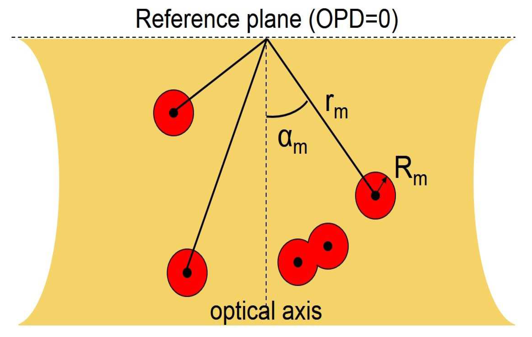
In the proposed method, each scatterer also representing a sub-surface feature of interest in SOCT is modeled as a multipole with boundaries formed by circles, semi-circles, connected circular arcs, or combinations of them, as shown in Figure 1. Specifically, we consider using M multipoles, each individual position is marked by, respectively, the radial distance and the azimuthal angle with reference to the center of the focusing lens in an OCT system. The light field detected at the focusing center can be expressed as the sum of scattered fields from the M multipoles as follows [13]:
where is the Bessel function of order n, and are unknown expansion coefficients, and is times the reciprocal of the wavelength.
Ignoring the self-correlation terms and DC terms due to the sample scattered spectrum and the mirror scattered spectrum, the depth resolved spectrum at the depth given by can be obtained by
where is the spectrum of the broadband light source used in the SOCT system.
The SOCT measurement can be expressed in the following compact format
where is a vector with elements of and for , and = .
It is noted that the model has factored into multiple scatterings. As shown in Section 3, multiple scatterings are contained only in the MMP terms of higher order. Hence, by removing the fields characterized by the high order terms from the SOCT measurement, the multiple scattering artifacts is removed from the SOCT results. Now, the problem of the proposed pre-processing method can be stated as the one of solving unknown parameters , , , and from the available . Once these unknowns are obtained, the pre-processed SOCT measurements are obtained by the summation in Equation (3) over those multipoles of pre-set orders.
For easy calculation, we take spectral measurements at different for and . L equations of unknowns are obtained as
where , , and . Equation (4) can be solved by the following optimization:
3. Effect of Multiple Scattering on MMP Expansion
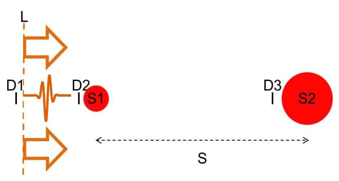
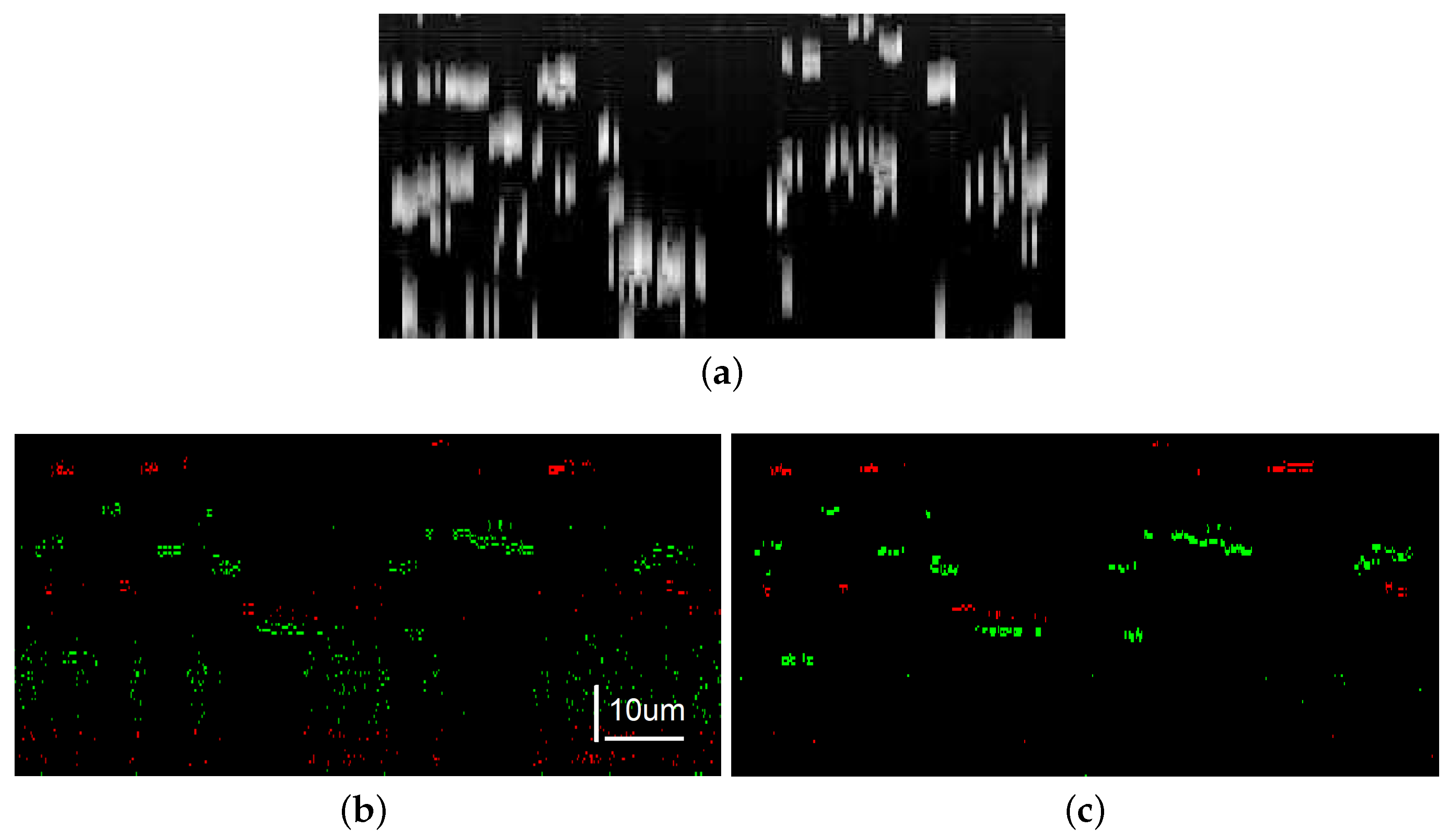
In this section, simulation studies are carried out to evaluate the contributions of multiple scatterings to the MMP expansion of SOCT measurements. We consider a sample with two spherical scatterers with diameters of 1 m and 4.5 m, respectively. The two scatterers are 10 m apart in space, as shown in Figure 2. The multiple scattering process is simulated in the following way. Assume a single light pulse of 6 fs starts from L and travels through the scatterers sequentially, we calculate the amplitudes of light fields at various positions and time using finite-difference time-domain (FDTD) method. This method is used to simulate the field distribution as it neither needs to assume the geometry of the scatterers nor the extent of multiple scattering. Thus, the method is able to consider the contributions of multiple scattering effectively in the calculated field distribution. We used commercial FDTD software (Lumerical) working in temporal mode to simulate the light fields over a time duration of 300 fs. Other simulation parameters included setting the maximum mesh size to 50 nm to ensure that the mesh size is smaller than the smallest wavelength used, and using perfectly matched layer (PML) boundary condition to terminate the field. Then, the simulation was run and the amplitudes at locations marked by D1, D2, and D3 are recorded at different time, as shown in Figure 3a.
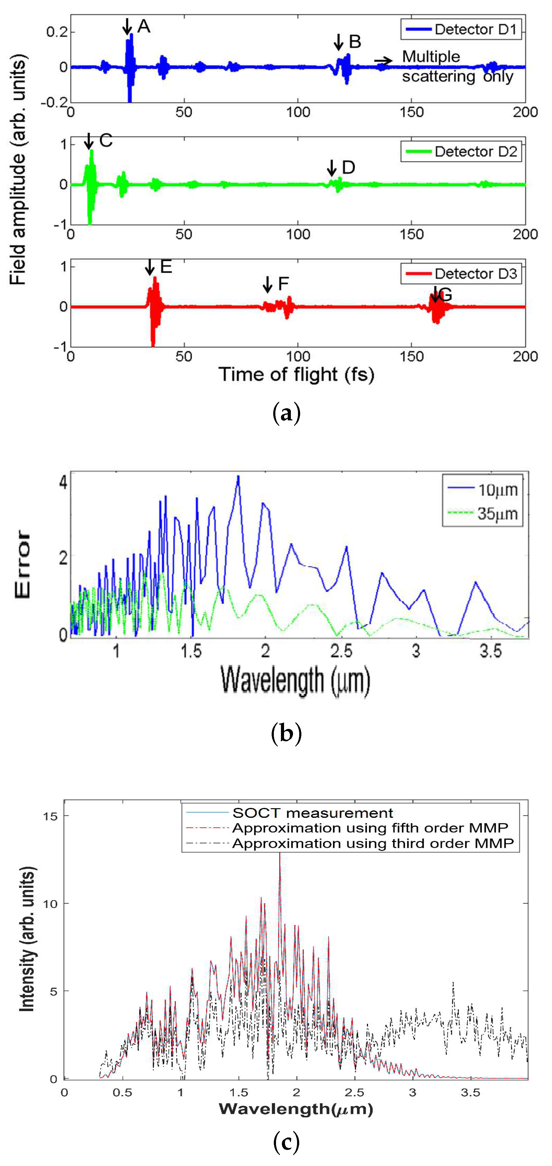
First, we considered the scattering events that contribute to the single scattered electric field received by D1. The light pulse first passes D2 and gives the response marked by C in Figure 3a, and then it encounters S1. One portion of the light is backscattered by S1 towards D1 and gives the response marked by A in Figure 3a. The other portion continues travelling towards D3 and gives a response marked by E in Figure 3a. After the light encounters S2, a portion of it carries on its forward propagation and does not return, whereas a backscattered portion travels towards D2. The backscattered portion propagates towards detector D2 and D1 and produces responses marked by D and B in Figure 3a, respectively. Beyond this instance, the scatterings that take place are multiple scattering fields and when the light pulse returns to D1, it generates the multiple scattering fields in SOCT measurement. Earlier when S1 is first illuminated by the light pulse, S1 scatters a portion of the field towards D3 to give the response F in Figure 3a. Likewise, the field described above that generates the response marked by D in Figure 3a is backscattered by S1 towards S2 to generate the response G in Figure 3a.
This process of scattering to and fro between spheres S1 and S2 goes on several times and gives the total field received at D1 containing both single and multiple scatterings. Thus, by filtering the response at D1 at different time durations, we can calculate, respectively, the spectrum due to electric field from single scattering and the spectrum due to the total received field including the multiple scattering portion. Furthermore, we can obtain the corresponding spectra. The difference between the two spectra is plotted in Figure 3b. For comparison, we repeated the simulation for the case when two scatterers are separated further by S = 35 m. The corresponding spectrum difference is included in the figure. The comparison clearly shows that the spectrum difference due to multiple scatterings becomes more significant when the two scatterers are closer. It is the spectrum difference that contributes the multiple scattering artifacts in SOCT.
Next, we show that MMP terms of higher order fit well the multiple scattering fields in SOCT measurements. We solve the optimization problem in Equation (5) on the SOCT measurements consisting of multiple scatterings using and , respectively. We take m, m, m … m] and . The resultant SOCT measurements are shown in Figure 3c. It is evident that the MMP terms of higher order can be used to characterize effectively the multiple scattering artifacts in the SOCT measurements. Hence, it is possible to filter the multiple scattering fields in SOCT measurements by limiting the order of the multiple multipole expansion. The filtered SOCT measurements from Equation (5) can then be used to calculate the depth resolved spectroscopy of SOCT.
4. Experiments and Discussions
4.1. Setup
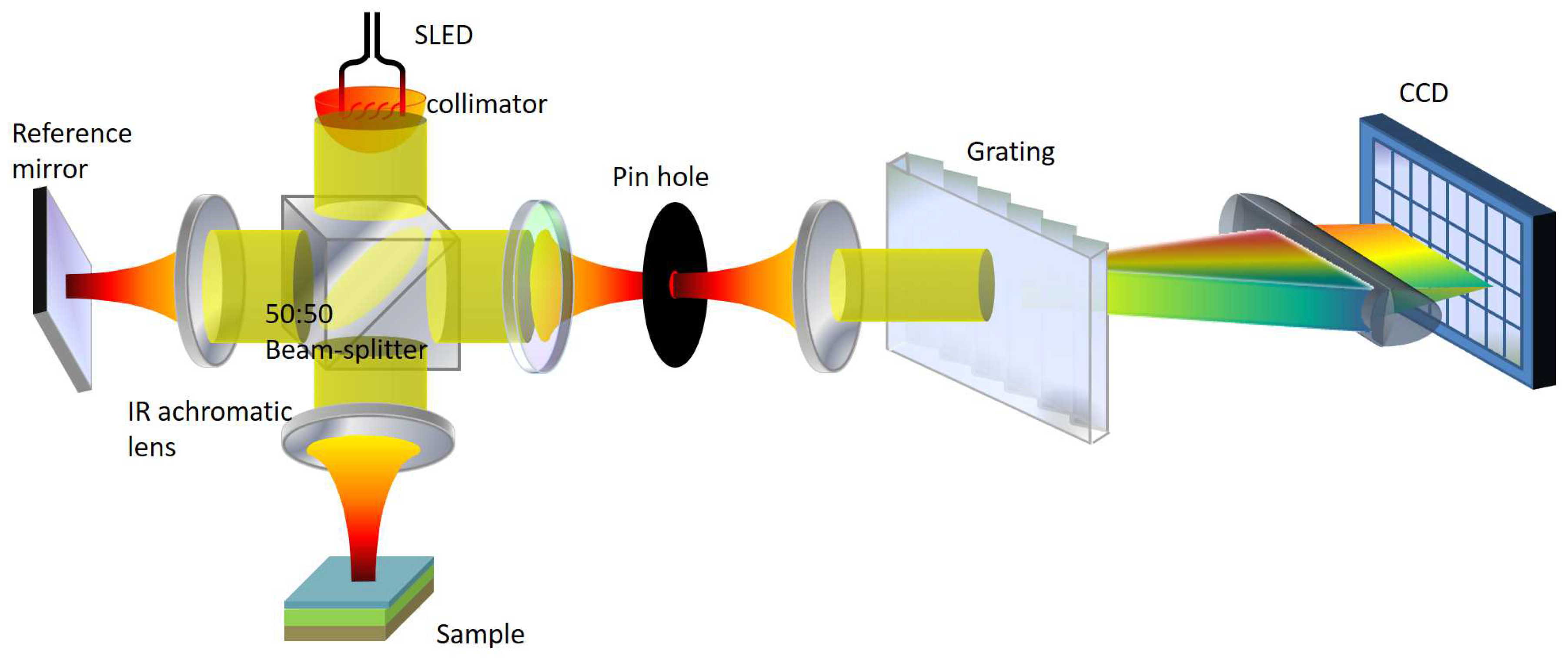
The performance of the proposed method was evaluated in an experiment by imaging a homemade phantom with an OCT setup, as shown in Figure 4. The OCT setup is a typical Michelson interferometer. Low coherence light comes from a superluminescent diode (QSDM-810-2, QPhotonics, Ann Arbor, USA) with center wavelength of 813 nm and FWHM linewidth of 19 nm. The light enters the interferometer via a collimator (NA = 0.26, Thorlabs, New Jersey, USA) and it is split into two paths by a 50:50 beam splitter (25 mm near-infrared non-polarizing cube beam-splitter, Edmund Optics, Singapore). The split light is then focused, respectively, on the reference mirror and the sample through near infrared achromatic lens (40 mm focal length, Edmund Optics, Singapore). The light reflected from the mirror and from the sample interferes again at the beam splitter. The interference light goes through a collimation module consisting of two identical achromatic lens with a m pinhole placed in the middle at the common focal point of two lenses. The collimated light is dispersed and projected to a charged coupled device (CCD, Dalsa 1M60, Waterloo, Canada) through a grating (800 lines per mm, Edmund Optics, Singapore), and an achromatic lens. A separate calibration shows the axial and lateral resolutions of the OCT setup are m and m, respectively.
4.2. Phantom
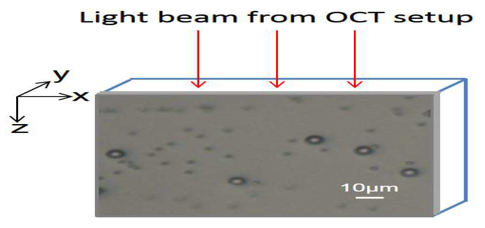
The homemade phantom was made by coating a film on a microscope glass slide. The film contains a mixture of microspheres with diameters of m and m microspheres. The film was made in the following steps. A thin layer of glue is first applied onto the surface of the microscope glass slide. Then, a L droplet of solution consisting of a mixture of polystyrene microspheres of m and m diameters is dropped onto the microscope glass slide. The droplet of solution is spread out by gently pressing a cover glass with a thin layer of glue facing down onto the surface of the microscope glass slide. A microscopy picture of the phantom is shown in Figure 5.
4.3. Imaging Procedures
In the experiment, we imaged the film from its side rather than its surface, as shown in Figure 5. We aligned the phantom along the Z-direction (not the X-direction) to the light beam of a typical SOCT setup. The spectra of A-scans in a cross-section of the sample were collected in a process of scanning the sample with a motorized translational stage (25 mm translational stage, Zaber, Vancouver, Canada). The scanning was done in steps of 1 m along the cross-section of interest. At every scan position, an A-scan spectrum was captured. A total of 500 A-scans were obtained for three cross-sections: the first cross-section contains only m diameter microspheres, the second one contains only m diameter microspheres, and the third one contains both m and m diameter microspheres.
Then, the proposed method was applied to process the A-scan spectra through solving the optimization problem in Equation (6) on the SOCT measurements by using , , m m, m … m] and . This solution provided us the estimates of the parameters for the scatterers, namely , , and . Then, we used these parameters to reconstruct the spectra reflected from each scatterer by using Equation (2). After this pre-processing, a short-time Fourier transform was performed on the processed A-scan spectra and we obtained a SOCT image by calculating the contrast measure described in the section below.
4.4. Visualization
For better visualization of the SOCT image, a new contrast measure is introduced here, and it is defined by . The measure reflects the scatterer size because both and in the MMP expansion are directly proportional to the radius of curvature of scatterer boundary. To display the SOCT image of the phantom, the contrast measure is rounded about two values that, respectively, represent the m and m diameter microspheres. The contrast is coded into the green and red channels. As a result, the image obtained by the proposed method are obtained. We also process the SOCT measurement by short-time Fourier transform method. The SOCT images for the cross-section containing only m diameter microspheres and the one containing only m diameter microspheres are shown in Figure 6 and Figure 7, respectively. The corresponding microscope images are also given for reference. Finally, we process in the same manner the SOCT measurement obtained from the cross-section containing a mixture of m and m diameter microspheres. We also process the SOCT measurements by the standard FD-OCT method and the short-time Fourier transform method. The obtained images are included in Figure 8 for comparison.
Comparing the SOCT images obtained by short-time Fourier transform method and the proposed method in Figure 6 and Figure 7, we can see that the images obtained by short-time Fourier transform displayed artifacts due to multiple scatterings when two scatterers that are located close together, whereas the SOCT image from the proposed method does not have this artifact.
Comparing the images in Figure 8 draws two observations. First, the proposed method can locate the scatterers of m and 2 m, as shown in Figure 5. Second, compared with the one obtained by short-time Fourier transform, the proposed method is able to eliminate the artifacts due to multiple scatterings. This can be attributed to the ability of the multiple multipole expansion to differentiate the multiple scatterings from single scatterings.
5. Conclusions
In summary, this paper uses a multiple multipole expansion method to model the light fields in a sample under SOCT imaging. Since OCT and SOCT setup uses the same set of measurement, the pre-processing method is also applicable to OCT. Using the proposed method, multiple scatterings from features in the sample can be effectively modeled by a parameterized optimization problem. With the parameters obtained, multiple scattering fields can be filtered out from the SOCT measurements before applying routine time–frequency analysis of SOCT. The multiple scattering artifacts are removed in the SOCT imaging results. Experiments on a calibrated phantom has exemplified that the proposed method can improve the image quality. The challenges to integrate this method to existing time–frequency analysis methods are with obtaining a suitable scattering model of the features and minimizing the spectral distortion that could arise from dispersion. In the case of industrial samples, suitable scattering models would be determined by characterizing the scattered spectra and dispersion of the different materials used to manufacture the samples.
Author Contributions
Conceptualization, Y.Z.; Data curation, H.L.S.; and Writing—review and editing: H.L.S. and Y.Z.
Funding
This research received funding support from Singapore Institute of Manufacturing Technology and A*Star.
Conflicts of Interest
The authors declare no conflict of interest.
References
- Morgner, U.; Drexler, W.; Kartner, F.X.; Li, X.D.; Pitris, C.; Ippen, E.P.; Fujimoto, J.G. Spectroscopic optical coherence tomography. Opt. Lett. 2000, 25, 111–113. [Google Scholar] [CrossRef] [PubMed]
- Adhi, M. Optical coherence tomography—Current and future applications. Curr. Opin. Ophthalmol. 2008, 24, 213–221. [Google Scholar] [CrossRef] [PubMed]
- Nam, H.S.; Yoo, H. Spectroscopic optical coherence tomography: A review of concepts and biomedical applications. Appl. Spectrosc. Rev. 2018, 53, 91–111. [Google Scholar] [CrossRef]
- Oldenburg, A.L.; Xu, C.; Boppart, S.A. Spectroscopic Optical Coherence Tomography and Microscopy. IEEE J. Sel. Top. Quantum Electron. 2007, 13, 1629–1640. [Google Scholar] [CrossRef]
- Zhou, Y.; Zhao, Y.; Kim, S.; Wax, A. Spectroscopic OCT: Towards an effective tool for distinguishing authentic and artifical Chinese freshwater pearls. Opt. Mater. Express 2018, 8, 622–628. [Google Scholar] [CrossRef]
- Nam, H.S.; Song, J.W.; Jang, S.J.; Lee, J.J.; Oh, W.Y.; Kim, J.W.; Yoo, H. Characterization of lipid-rich plaques using spectroscopic optical coherence tomography. J. Biomed. Opt. 2016, 7, 75004. [Google Scholar] [CrossRef] [PubMed]
- Graf, R.N.; Wax, A. Temporal coherence and time frequency distributions in spectroscopic optical coherence tomography. J. Opt. Soc. Am. A 2007, 24, 2186–2195. [Google Scholar] [CrossRef]
- Robles, F.E.; Wilson, C.; Grant, G.; Wax, A. Molecular imaging true-colour spectroscopic optical coherence tomography. Nat. Photonics 2008, 5, 744–747. [Google Scholar] [CrossRef] [PubMed]
- Nguyen, V.D.; Faber, D.J.; van der Pol, E.; van Leeuwen, T.G.; Kalkman, J. Dependent and multiple scattering in transmission and backscattering optical coherence tomography. Opt. Express 2013, 21, 29145–29156. [Google Scholar] [CrossRef] [PubMed]
- Wang, R.K. Signal degradation by multiple scattering in optical coherence tomography of dense tissue: A Monte Carlo study towards optical clearing of biotissues. Phys. Med. Biol. 2002, 47, 2281–2299. [Google Scholar] [CrossRef] [PubMed]
- Badon, A.; Li, D.; Lerosey, G.; Claude Boccara, A.; Fink, M.; Aubry, A. Smart optical coherence tomography for ultra-deep imaging through highly scattering media. Sci. Adv. 2016, 2, e1600370. [Google Scholar] [CrossRef] [PubMed]
- Liu, S.; Lamont, M.R.E.; Mulligan, J.; Adie, S.G. Aberration-diverse optical coherence tomography for suppression of multiple scattering and speckle. Biomed. Opt. Express 2018, 10, 4919–4935. [Google Scholar] [CrossRef]
- Hafner, C. Multiple multipole programs (MMP). In The Generalized Multipole Technique for Computational Electromagnetics; Artech House Books: London, UK, 2007; pp. 219–265. [Google Scholar]
Figure 1.
Schematic illustration of an A-scan.

Figure 2.
Schematic illustration of an A-scan showing the locations of optical axis and reference plane. The reference plane has zero optical path difference (OPD) with the reference mirror in OCT setup.
Figure 2.
Schematic illustration of an A-scan showing the locations of optical axis and reference plane. The reference plane has zero optical path difference (OPD) with the reference mirror in OCT setup.

Figure 3.
(a) Schematic of a single pulse light travelling in a sample consisting of the two scatterers; (b) spectra error; and (c) spectra obtained using MMP terms of different order.Simulation of the multiple scattering artifacts
Figure 3.
(a) Schematic of a single pulse light travelling in a sample consisting of the two scatterers; (b) spectra error; and (c) spectra obtained using MMP terms of different order.Simulation of the multiple scattering artifacts

Figure 4.
Schematic illustration of the OCT setup and the components used.

Figure 5.
Cross-sectional view of the phantom sample imaged by Olympus upright microscope with 100× magnification (the while bar denotes 10 m).
Figure 5.
Cross-sectional view of the phantom sample imaged by Olympus upright microscope with 100× magnification (the while bar denotes 10 m).

Figure 6.
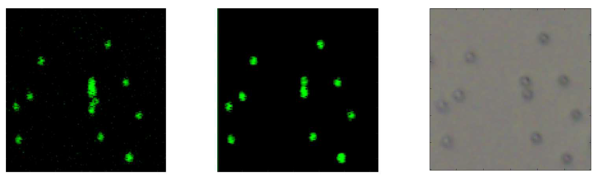
Imaging of the cross-section with m microspheres only: (Left) SOCT image of the cross-section obtained by short-time Fourier transform method; (Middle) SOCT image of the cross-section obtained by the proposed method; and (Right) cross-sectional view of the area under investigation. SOCT images are normalized and displayed in logarithmic scale.
Figure 6.
Imaging of the cross-section with m microspheres only: (Left) SOCT image of the cross-section obtained by short-time Fourier transform method; (Middle) SOCT image of the cross-section obtained by the proposed method; and (Right) cross-sectional view of the area under investigation. SOCT images are normalized and displayed in logarithmic scale.

Figure 7.
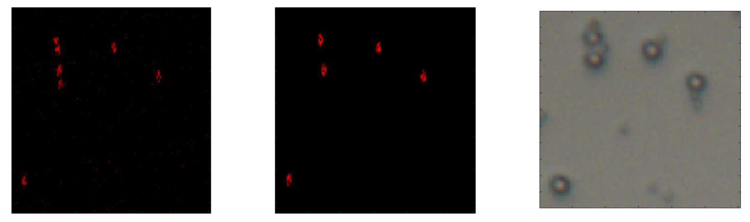
Imaging of the cross-section with m microspheres only: (Left) SOCT image of the cross-section obtained by short-time Fourier transform method; (Middle) SOCT image of the cross-section obtained by the proposed method; and (Right) cross-sectional view of the area under investigation. SOCT images are normalized and displayed in logarithmic scale. In the microscope image, there are small air bubbles that are not in the imaging XZ plane and they do not contribute our SOCT measurement.
Figure 7.
Imaging of the cross-section with m microspheres only: (Left) SOCT image of the cross-section obtained by short-time Fourier transform method; (Middle) SOCT image of the cross-section obtained by the proposed method; and (Right) cross-sectional view of the area under investigation. SOCT images are normalized and displayed in logarithmic scale. In the microscope image, there are small air bubbles that are not in the imaging XZ plane and they do not contribute our SOCT measurement.

Figure 8.
Cross-sectional images of the phantom sample obtained by the: (a) FD-OCT method; (b) short-time Fourier transform; and (c) the proposed method with short-time Fourier transform. Images are normalized and displayed in logarithmic scale.Phantom sample imaging
Figure 8.
Cross-sectional images of the phantom sample obtained by the: (a) FD-OCT method; (b) short-time Fourier transform; and (c) the proposed method with short-time Fourier transform. Images are normalized and displayed in logarithmic scale.Phantom sample imaging

© 2018 by the authors. Licensee MDPI, Basel, Switzerland. This article is an open access article distributed under the terms and conditions of the Creative Commons Attribution (CC BY) license (http://creativecommons.org/licenses/by/4.0/).
Share and Cite
MDPI and ACS Style
Seck, H.L.; Zhang, Y. Spectroscopic Optical Coherence Tomography by Using Multiple Multipole Expansion. Photonics 2018, 5, 44. https://doi.org/10.3390/photonics5040044
AMA Style
Seck HL, Zhang Y. Spectroscopic Optical Coherence Tomography by Using Multiple Multipole Expansion. Photonics. 2018; 5(4):44. https://doi.org/10.3390/photonics5040044
Chicago/Turabian StyleSeck, Hon Luen, and Ying Zhang. 2018. "Spectroscopic Optical Coherence Tomography by Using Multiple Multipole Expansion" Photonics 5, no. 4: 44. https://doi.org/10.3390/photonics5040044
Note that from the first issue of 2016, this journal uses article numbers instead of page numbers. See further details here.