Communication

Denoising of Laser Self-Mixing Interference by Improved Wavelet Threshold for High Performance of Displacement Reconstruction

1
School of Mechanical and Electrical Engineering, Xi’an Polytechnic University, Xi’an 710600, China
2
Focuslight Technologies Inc., Xi’an 710077, China
*
Author to whom correspondence should be addressed.
These authors contributed equally to this work.
Photonics 2023, 10(8), 943; https://doi.org/10.3390/photonics10080943
Submission received: 25 July 2023 / Revised: 10 August 2023 / Accepted: 15 August 2023 / Published: 18 August 2023
(This article belongs to the Special Issue Advanced Photonic Sensing and Measurement)

Abstract

:
This article proposes an improved wavelet threshold denoising for laser self-mixing interference signals. The improved wavelet threshold function exhibits smoothness and continuity near the threshold. By replacing hard or soft wavelet threshold with the improved wavelet threshold, it can eliminate the generation of fake self-mixing interference peaks due to local oscillation induced by hard wavelet threshold, as well as the loss of self-mixing interference peaks due to over-smoothness induced by the soft wavelet threshold. Compared with hard and soft wavelet threshold denoising, theoretical simulations and experimental results demonstrate that the displacement of vibrations are well reconstructed based on the improved wavelet threshold denoising.

1. Introduction

In recent years, the application of laser self-mixing interferometry in micro-displacement measurement has gained significant attention [1,2,3,4,5]. Laser self-mixing interferometry offers several advantages over traditional micro-displacement measurement techniques, including no optical interferometer external to the source, no external photodetector, non-contact operation, high sensitivity, high precision, environmental insensitivity, and high resolution [6,7,8,9,10,11]. As a result, laser self-mixing interferometry has emerged as a prominent research area in micro-displacement measurement [8,9,10]. For self-mixing in a diode laser, the small backreflected field phasor Er re-enters the laser cavity and it adds to the lasing field phasor E0. The phase of Er is φ(t) = 2ks(t), where k = 2π/λ and s(t) is the distance of the remote target. Hence, the lasing field amplitude and frequency are modulated by the term φ(t) = 2ks(t) [11]. Power fluctuations ΔP in the steady-state operation of the LD in the weak feedback regime follow the equation: ΔP~cos(φ(t)) [6]. In practical measurement scenarios, the presence of various sources of noise, such as ambient temperature, fluctuation in the LD driving source and other disturbances, can be introduced into self-mixing interference (SMI) signals [12,13]. When the noise exists in the SMI signals, it will introduce random disturbance on the phase leading to the instability and inaccuracy of the displacement reconstruction. Yoshino et al., have used complex electrical feedback techniques to eliminate the external disturbances to measure vibration or displacement of the object [14]. Currently, several algorithms are used for denoising in SMI signals, including FFT phase denoising [15,16], variational mode decomposition (VMD) denoising [17,18], and wavelet threshold denoising [19].
The wavelet threshold denoising algorithm offers the advantage of retaining signal characteristics [19]. The wavelet transform-based denoising method, which can effectively eliminate noise while keeping an SMI waveform less changed [13]. In this algorithm, the signals are decomposed into wavelet coefficients at different scales through multiscale analysis and subsequently performed denoising based on the set of the threshold function [20]. Generally, the set of the soft and hard thresholds have a significant impact on the wavelet denoising results [21,22]. Zhao Y. et al., used a continuous wavelet transform to remove noise from SMI signals [23]. Bernal O. D. et al., used two different mother wavelets to distinguish between the SM mode and displacement direction [24]. However, the wavelet denoising algorithm using soft and hard threshold functions encounters challenges in achieving a high performance of SMI displacement reconstruction, in which the loss of signals and the generation of fake signals happens by using soft and hard threshold functions, respectively [25,26,27].
This article proposes an improved wavelet threshold denoising for laser self-mixing interference signals. The improved wavelet threshold function exhibits smoothness and continuity near the threshold. By replacing hard or soft wavelet threshold with the improved wavelet threshold, it can eliminate the generation of fake self-mixing interference peaks due to local oscillation induced by the hard wavelet threshold, as well as the loss of self-mixing interference peaks due to over-smoothness induced by the soft wavelet threshold. Compared with hard and soft wavelet threshold denoising, theoretical simulations and experimental results demonstrate that the displacement of vibrations are well reconstructed based on the improved wavelet threshold denoising.

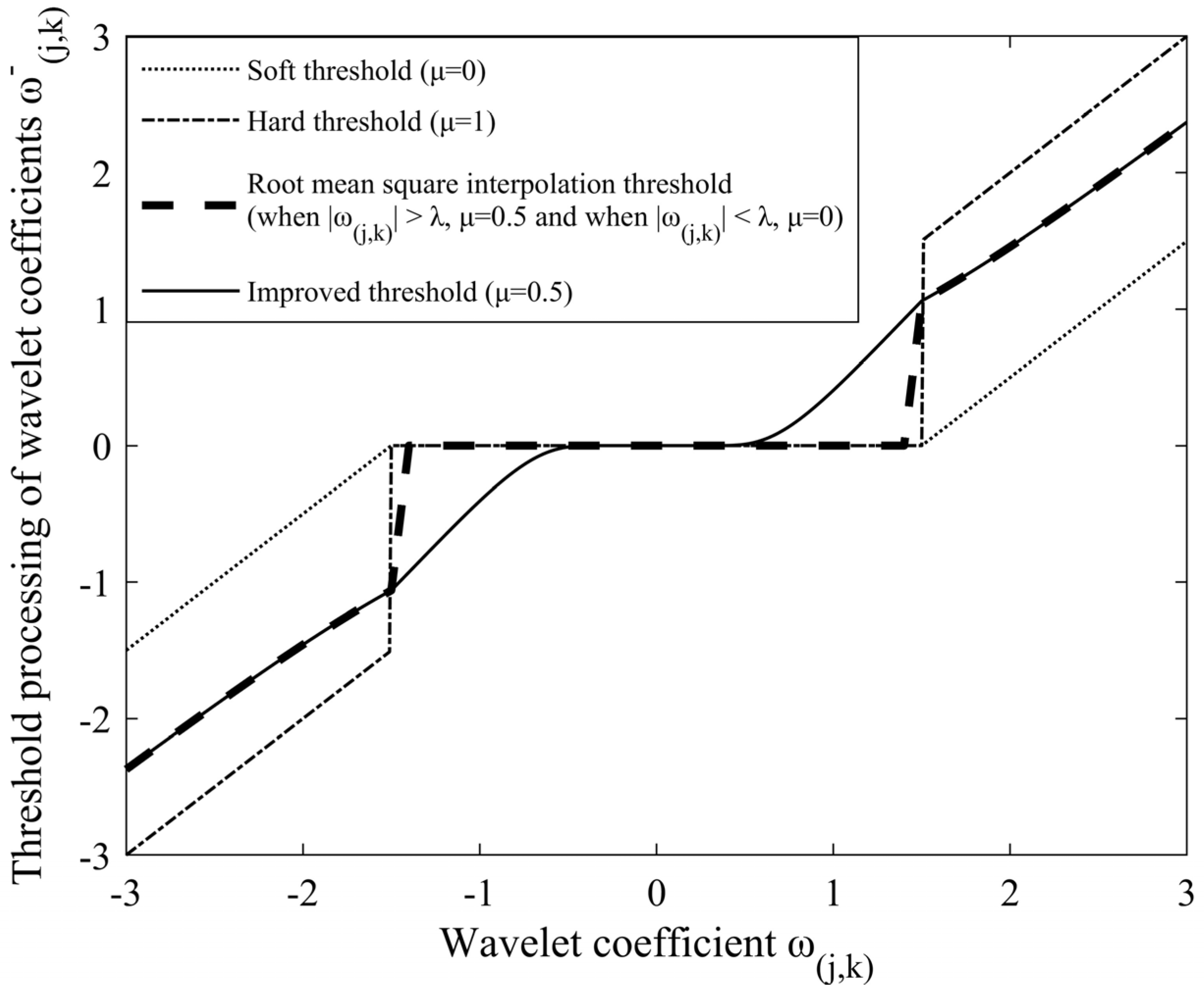
2. Improved Wavelet Threshold Denoising Function

In the wavelet threshold denoising algorithm, the threshold function is utilized to perform threshold denoising on the detail component coefficients obtained from the n-layer wavelet decomposition of the signal, yielding estimated wavelet coefficients [28].
Based on the root-mean-square interpolation threshold function [29], an improved wavelet threshold function in wavelet denoising is introduced here. The improved threshold function is described as follows:
ω ^ j , k = sgn ( ω j , k ) μ ω j , k 2 + ( 1 μ ) ( | ω j , k | λ ) 2 | ω j , k | λ μ ω j , k e 1 λ 2 1 ω j , k 2 | ω j , k | < λ
where ω j , k and ω ^ j , k correspond to the wavelet coefficients before and after quantization processing, respectively; j is the scale parameter, and k is the translation parameter; sgn ( * ) is symbolic piecewise function; the wavelet threshold function can be adjusted by changing the parameter μ ( μ [ 0 , 1 ] ); and the threshold λ is determined by
λ = σ 2 ln N
where σ is the noise standard deviation, and N is the length of the signal.
Figure 1 shows the profiles of different wavelet threshold functions with different μ in Equation (1). The value of threshold λ here is calculated as 1.5 based on the simulated SMI signals shown in Part 3 according to Equation (2). When μ is 0, Equation (1) is reduced to soft wavelet threshold function represented by dotted line in Figure 1; when μ is 1, Equation (1) is reduced to hard wavelet threshold function represented by dash dotted line in Figure 1. For the absolute value of ω j , k higher than the threshold λ in Figure 1, the profile of the root-mean-square interpolation threshold function and improved wavelet threshold function are overlapped, which can overcome the over-smoothness in wavelet threshold denoising with soft wavelet threshold function. For the absolute value of ω j , k lower than the threshold λ in Figure 1, the profile of the improved threshold function exhibits continuity near the threshold, which can overcome local oscillation in wavelet threshold denoising with the hard threshold and root-mean-square interpolation threshold.

3. Theoretical Simulation and Analysis

3.1. Simulation of Laser SMI Signals

Assume that the object vibrates near the zero point with sinusoidal oscillation, the SMI signals for the object vibration can be simulated by the method in [30]. The parameters used in numerical simulation are shown in Table 1.
Figure 2a shows the result of the simulation profile of object vibration; Figure 2b shows the result of the simulation profile of SMI signals. In Figure 2b, the curve is divided by dashed lines with the time interval 0.05 s. The hollow stars and solid stars represent the peak and valley points in SMI simulation signal, respectively. The numbers of peak and valley values in each divided part are both 12. The random noise with 10 dB is added to SMI signals and the result is shown in Figure 2c, which is used as the wavelet denoising target with different wavelet threshold functions shown in Figure 1.

3.2. Simulation of Different Wavelet Threshold Denoising

The SMI signals are decomposed into the target layers by the wavelet threshold de-noising algorithm, in which the low-frequency approximate coefficients and the high-frequency detail coefficients are obtained. The coefficients component of wavelet de-composition for the SMI signals in Figure 2c are shown in Figure 3. The low-frequency approximate coefficients shown in Figure 3a keep the characteristics of the SMI signal. The wavelet threshold function shown in Figure 1 are used to filter the high-frequency detail coefficients shown in Figure 3b–g.
Consequently, the low frequency approximate component and filtered high frequency detail component are used to obtain the reconstructed SMI signal by inverse wavelet transform, the results of reconstructed SMI signal are shown in Figure 4.
As can be seen in Figure 4, Figure 4a shows the reconstructed SMI signals using soft wavelet threshold denoising; Figure 4b shows the reconstructed SMI signals using hard wavelet threshold denoising; and Figure 4c shows the reconstructed SMI signals using improved wavelet threshold denoising. The hollow stars represent the peak points of the re-constructed SMI signals; the solid stars represent the valley points of the reconstructed SMI signals. The number of peak and valley points in the reconstructed SMI signals are also shown in Figure 4. The number of peak and valley points near and at phase jump points of the SMI signal are excluded.
Compared with simulated SMI signals in Figure 2b, loss of SMI valley occurs near 0.16 s using soft wavelet threshold function, which can be seen in Figure 4a; fake SMI peaks happen using the hard wavelet threshold function, which can been seen in Figure 4b. The loss of the SMI valley and generation of fake SMI peak directly influence the displacement reconstructed accuracy. Based on the improved wavelet threshold function in SMI signals denoising shown in Figure 4c, the number of peaks and valleys in SMI signals located within each phase jump point is 12, which is the same as that shown in Figure 2b.

3.3. Comparison of Displacement Reconstruction for the Simulated SMI

The displacement reconstruction is conducted by the phase unwrapping algorithm for the SMI signals. Figure 5 illustrates the comparison between the simulated object vibration signal and the displacement reconstruction from filtered SMI signals by different wavelet threshold functions for denoising shown in Figure 4.
It can be seen from Figure 5a that the curve of the reconstructed displacement by soft wavelet threshold denoising deviates from simulated object vibration signal after 0.15 s, in which the maximum deviation of the reconstructed displacement is 18.26%. This is attributed to the over smoothness and induces the loss of valleys in SMI signals.
As is shown in Figure 5b, great deviations happen for the phase jump points at 0.05 s and 0.15 s, and the maximum reconstruction displacement deviation is 20.94%. This is attributed to the local oscillation phenomenon by using hard wavelet threshold, in which fake SMI peaks are induced in the denoised SMI signal.
In contrast, Figure 5c illustrates that the curve of the reconstructed displacement using de-noised SMI by improved wavelet threshold are consistent with that of the simulated object vibration. The maximum displacement deviation in vibration reconstruction is only 1.07%.

4. Experiment of Improved Wavelet Threshold Denoising in SMI Signals

4.1. Laser SMI Experimental Setup and Results

The laser self-mixing interference experimental system consists of three modules: simulated vibration source, beam transmission, and data acquisition. A semiconductor laser with a wavelength of 635 nm is selected as the light source. The emitted light is reflected by piezoelectric ceramics (PZT). A piezoelectric controller (ThorlabsKPZ101) is used to drive the PZT to generate micro-displacement Lext. The error resulted from the non-linear reaction of PZT and surrounding mechanical disturbance can be ignored [31]. The driving current of the laser diode controller (ThorlabsLDC205C) was used to set the working current of the semiconductor laser, and the mechanical translation platform was used to adjust the length of the external cavity. The SMI signal is converted and amplified by the current–voltage circuit, and the data acquisition card (NIUSB-6341) is used for data acquisition, and the SMI signal waveform is displayed on the computer in real time. The details of the experimental setup are given in reference [6]. In this experiment, the external cavity length is 33.9 mm, the modulation frequency is 10 Hz, and the modulation amplitude is 2 V. The power of the diode laser in operation is about 3 mW. The bandwidth and noise of the detection chain are 1.2 MHz and 135 μV, respectively. The amplitude of displacement of the PZT mirror is about 5.5 μm. The SNR of the detected signal after SMI is 100:1. And the PZT is driven to generate the sinusoidal motion. The vibrating back-scattering light from the PZT mirror can influence the SMI signals. In the process of the experiment, the effect of the vibrating back-scattering light on the SMI signals can be largely eliminated by adjusting the external cavity to decrease the scattering light to couple into the diode laser. It can make sure that the paraxial light beam goes back into diode laser. The experimental results of SMI signals are shown in Figure 6. The noises in SMI signals shown, e.g., in Figure 6b originated from electrical noise induced by the voltage fluctuation of the data acquisition card and the optical noise induced by the fluctuation of the laser output light power.

4.2. Denoising for SMI Based on Wavelet Threshold Function

The wavelet threshold function shown in Figure 7 are used in SMI signal denoising, in which the threshold λ is calculated as 0.16 here according to Equation (2) and μ is set as 0.35 for the experimental SMI signals shown in Figure 6b.
The experimental SMI signals are decomposed by the wavelet, which are shown in Figure 8. Figure 8a shows the low-frequency approximate coefficient of the SMI signal, and Figure 8b–g show the high-frequency detail coefficients. The profile of the low-frequency approximate coefficients keeps the characteristics of the SMI signal. The high-frequency detail component of the SMI noisy signal is filtered by the wavelet threshold function shown in Figure 7. Consequently, the filtered high-frequency detail component and low-frequency approximate component are used to obtain the reconstructed SMI signal by inverse wavelet transformation; the results of reconstructed SMI signal are shown in Figure 9.
Figure 9 shows the denoising results of the experimental SMI signals shown in Figure 6 using the different wavelet threshold denoising functions shown in Figure 7. Figure 9a shows the reconstructed SMI signals using soft wavelet threshold denoising; Figure 9b shows the reconstructed SMI signals using hard wavelet threshold denoising; and Figure 9c shows the reconstructed SMI signals using improved wavelet threshold denoising.
As can be seen from Figure 9a, the reconstructed profile for the denoised experimental SMI signals is distorted from the experimental SMI signals shown in Figure 6, which is attributed to the excessive smoothing with wavelet soft threshold denoising. In Figure 9b, the generation of the fake SMI peak or valley happens, which is attributed to local oscillation induced by the discontinuity with the wavelet hard threshold denoising function.

4.3. Comparison of Displacement Reconstruction for Experimental SMI

The displacement reconstruction is conducted by the phase unwrapping algorithm for the SMI signals shown in Figure 9. Figure 10 illustrates the comparison between the normalized driving voltage on PZT (represented by the solid line) and the normalized reconstruction displacement from experimental SMI signals or filtered experimental SMI signals.
The total measurement time needed to interrogate one cycle deformation in Figure 10 is about 4 s. The displacement interrogation mainly contains two processes: (1) the reconstruction of the SMI signal by inverse wavelet transform; and (2) displacement reconstruction by phase unwrapping algorithm. For the experimental SMI signals, the results of displacement interrogation based on above two processes are nearly the same.
From Figure 10a, the normalized displacement profile is reconstructed from the experimental SMI signals, which is deviated from the profile of the normalized PZT driving voltage. These deviations are attributed to the influence of SMI noise in the process of displacement reconstruction by the phase unwrapping algorithm, which affects the accuracy and stability of the reconstruction.
The profile of the normalized displacement in Figure 10b–d is reconstructed from the experimental filtered SMI signals, which are obtained based on soft wavelet threshold denoising, hard wavelet threshold denoising, and improved wavelet threshold denoising. In Figure 10b, the curve of the displacement reconstruction near 0.15 s is obviously deviated from the profile of the normalized PZT driving voltage, in which the maximum deviation between the two curves is 4.72%. In Figure 10c, the curve of displacement reconstruction near 0.05 s and 0.19 s are obviously deviated from the profile of the normalized PZT driving voltage, in which the maximum deviation between the two curves is 9.78%. In Figure 10d, the curve of the displacement reconstruction highly overlaps with the profile of the normalized PZT driving voltage.
It demonstrates that the improved wavelet threshold denoising function can eliminate the generation of fake self-mixing interference signals due to local oscillation caused by hard wavelet thresholds, as well as the loss of self-mixing interference signals due to over-smoothness caused by the soft threshold.

5. Conclusions

This article proposes an improved wavelet threshold denoising for laser self-mixing interference signals. The improved wavelet threshold function exhibits smoothness and continuity near the threshold. By replacing hard or soft wavelet threshold with the improved wavelet threshold, it can eliminate the generation of fake self-mixing interference peaks due to local oscillation induced by the hard wavelet threshold, as well as the loss of self-mixing interference peaks due to over-smoothness induced by the soft wavelet threshold. The simulation illustrates that the maximum deviation of the reconstructed displacement is 18.26% and 20.94% based on the filtered SMI signals by soft and hard wavelet threshold denoising, respectively; the experiment demonstrates the maximum deviation of the reconstructed displacement is about 5% and 9%. Compared with hard and soft wavelet threshold denoising, theoretical simulations and experimental results demonstrate that the displacement of vibrations are well reconstructed based on the improved wavelet threshold denoising.

Author Contributions

Conceptualization, H.L. and Y.Y.; methodology, H.L. and Y.Y.; validation, Y.Y.; data curation, S.L.; writing—original draft preparation, Y.Y.; writing—review and editing, H.L., D.H. (Dan He) and J.S.; and supervision, J.W. and D.H. (Dong Hou). All authors have read and agreed to the published version of the manuscript.

Funding

This research was funded by the Project supported by the QINCHUANGYUAN “Engineer plus Scientist” Team of Shannxi Province of China (grant number 2023KXJ-129) and the Natural Science Basic Research Plan in Shaanxi Province of China (grant number 2022JM-362).

Institutional Review Board Statement

Not applicable.

Informed Consent Statement

Not applicable.

Data Availability Statement

The data underlying the results presented in this paper are not publicly available at this time but may be obtained from the authors upon reasonable request.

Conflicts of Interest

The authors declare no conflict of interest.

References

  1. Alexandrova, A.S.; Tzoganis, V.; Welsch, C.P. Laser diode self-mixing interferometry for velocity measurements. Opt. Eng. 2015, 54, 034104. [Google Scholar] [CrossRef]
  2. Zhang, Z.; Li, C.; Huang, Z. Vibration measurement based on multiple Hilbert transform for self-mixing interferometry. Opt. Commun. 2019, 436, 192–196. [Google Scholar] [CrossRef]
  3. Zabit, U.; Bosch, T.; Bony, F. Adaptive transition detection algorithm for a self-mixing displacement sensor. IEEE Sens. J. 2009, 9, 1879–1886. [Google Scholar] [CrossRef]
  4. Donatia, S.; Norgiab, M. Overview of self-mixing interferometer applications to mechanical engineering. Opt. Eng. 2018, 57, 051506. [Google Scholar]
  5. Lu, L.; Yang, J.; Zhai, L.; Wang, R.; Cao, Z.; Yu, B. Self-mixing interference measurement system of a fiber ring laser with ultra-narrow linewidth. Opt. Express 2012, 20, 8598–8607. [Google Scholar] [CrossRef] [PubMed]
  6. Liu, H.; Li, S.; You, Y.; Wang, J.; Sun, J.; Zhang, L.; Xiong, L. Model of multiple mode gain competition in self-mixing laser diode. Optik 2023, 281, 170853. [Google Scholar] [CrossRef]
  7. Zheng, W.; Huang, W.; Zhang, J.; Wang, X.; Zhu, H.; An, T.; Yu, X. Obtaining scalable fringe precision in self-mixing interference using an even-power fast algorithm. IEEE Photonics J. 2017, 9, 6803211. [Google Scholar]
  8. Donati, S. Developing self-mixing interferometry for instrumentation and measurements. Laser Photonics Rev. 2012, 6, 393–417. [Google Scholar] [CrossRef]
  9. Wang, X.F.; Yuan, Y.; Sun, L.; Gao, B.; Chen, P. Self-mixing interference displacement measurement under very weak feedback regime based on integral reconstruction method. Opt. Commun. 2019, 445, 236–240. [Google Scholar] [CrossRef]
  10. Bes, C.; Plantier, G.; Bosch, T. Displacement measurements using a self-mixing laser diode under moderate feedback. IEEE Trans. Instrum. Meas. 2006, 55, 1101–1105. [Google Scholar] [CrossRef]
  11. Giuliani, G.; Norgia, M.; Donati, S.; Bosch, T. Laser diode self-mixing technique for sensing applications. J. Opt. A Pure Appl. Opt. 2002, 4, S283–S294. [Google Scholar] [CrossRef]
  12. Yu, Y.; Xi, J.; Chicharo, J.F. Improving the performance in an optical feedback self-mixing interferometry system using digital signal pre-processing. In Proceedings of the 2007 IEEE International Symposium on Intelligent Signal Processing, Alcala de Henares, Spain, 3–5 October 2007. [Google Scholar]
  13. Sun, Y.; Yu, Y.G.; Xi, J.T. Wavelet transform based de-noising method for self mixing interferometry signals. Proc. SPIE 2012, 8351, 83510G. [Google Scholar]
  14. Yoshino, T.; Nara, M.; Mnatzakanian, S.; Lee, B.S.; Strand, T.C. Laser diode feedback interferometer for stabilization and displacement measurements. Appl. Opt. 1987, 26, 892–897. [Google Scholar] [CrossRef] [PubMed]
  15. Wang, M. Fourier transform method for self-mixing interference signal analysis. Opt. Laser Technol. 2001, 33, 409–416. [Google Scholar] [CrossRef]
  16. Kou, K.; Wang, C.; Liu, Y. All-phase FFT based distance measurement in laser self-mixing interferometry. Opt. Laser Eng. 2021, 142, 106611. [Google Scholar] [CrossRef]
  17. Zhao, Y.; Zhang, B.F.; Han, L.F. Laser self-mixing interference displacement measurement based on VMD and phase unwrapping. Opt. Commun. 2020, 456, 124588. [Google Scholar] [CrossRef]
  18. Hua, T.; Dai, K.; Zhang, X.; Yao, Z.; Wang, H.; Xie, K.; Feng, T.; Zhang, H. Optimal VMD-based signal denoising for laser radar via Hausdorff distance and wavelet transform. IEEE Access 2019, 7, 167997–168010. [Google Scholar] [CrossRef]
  19. Wang, C.L.; Zhang, C.L.; Zhang, P.T. Denoising algorithm based on wavelet adaptive threshold. Phys. Procedia 2012, 24, 678–685. [Google Scholar]
  20. Bayer, F.M.; Kozakevicius, A.J.; Cintra, R.J. An iterative wavelet threshold for signal denoising. Signal Process. 2019, 162, 10–20. [Google Scholar] [CrossRef]
  21. Zhang, Y.; Ding, W.; Pan, Z.; Qin, J. Improved wavelet threshold for image de-noising. Front. Neurosci. 2019, 13, 39. [Google Scholar] [CrossRef]
  22. Liu, H.; Wang, W.D.; Xiang, C.; Han, L.; Nie, H. A de-noising method using the improved wavelet threshold function based on noise variance estimation. Mech. Syst. Signal Process. 2018, 99, 30–46. [Google Scholar] [CrossRef]
  23. Zhao, Y.; Li, J.; Zhang, M.; Zhao, Y.; Zou, J.; Chen, T. Phase-unwrapping algorithm combined with wavelet transform and Hilbert transform in self-mixing interference for individual microscale particle detection. Chin. Opt. Lett. 2023, 21, 041204. [Google Scholar] [CrossRef]
  24. Bernal, O.D.; Seat, H.C.; Zabit, U.; Surre, F.; Bosch, T. Robust fringe detection based on bi-wavelet transform for self-mixing displacement sensor. In Proceedings of the 2015 IEEE Sensors, Busan, Republic of Korea, 1–4 November 2015. [Google Scholar]
  25. Han, G.; Xu, Z. Electrocardiogram signal denoising based on a new improved wavelet thresholding. Rev. Sci. Instrum. 2016, 87, 084303. [Google Scholar] [CrossRef] [PubMed]
  26. Qian, Y. Image denoising algorithm based on improved wavelet threshold function and median filter. In Proceedings of the 2018 IEEE 18th International Conference on Communication Technology (ICCT), Chongqing, China, 8–11 October 2018. [Google Scholar]
  27. Zeng, Y.Q.; Zhang, B.C.; Zhao, W.; Xiao, S.; Zhang, G.; Ren, H.; Zhao, W.; Peng, Y.; Xiao, Y.; Lu, Y.; et al. Magnetic resonance image denoising algorithm based on cartoon, texture, and residual parts. Comput. Math. Method Med. 2020, 2020, 1405647. [Google Scholar] [CrossRef]
  28. Lu, J.Y.; Lin, H.; Ye, D.; Zhang, Y. A new wavelet threshold function and denoising application. Math. Probl. Eng. 2016, 2016, 3195492. [Google Scholar]
  29. Yang, K.; Deng, C.X.; Chen, Y.; Xu, L. The de-noising method of threshold function based on wavelet. In Proceedings of the 2014 International Conference on Wavelet Analysis and Pattern Recognition, Lanzhou, China, 13–16 July 2014. [Google Scholar]
  30. Kliese, R.; Taimre, T.; ABakar, A.A.; Lim, Y.L.; Bertling, K.; Nikolić, M.; Perchoux, J.; Bosch, T.; Rakić, A.D. Solving self-mixing equations for arbitrary feedback levels: A concise algorithm. Appl. Opt. 2014, 53, 3723–3736. [Google Scholar] [CrossRef]
  31. Wang, H.; Ruan, Y.X.; Yu, Y.G.; Guo, Q.H.; Xi, J.T.; Tong, J. A new algorithm for displacement measurement using self-mixing interferometry with modulated injection current. IEEE Access 2020, 8, 123253–123261. [Google Scholar] [CrossRef]
Figure 1. Different wavelet threshold denoising function (dotted line: soft wavelet threshold; dash dotted line: hard wavelet threshold; double line: root mean square interpolation threshold; and solid line: improved wavelet threshold.).
Photonics 10 00943 g001
Figure 2. (a) Simulated displacement of object vibration; (b) normalized intensity of simulated SMI (peak point marked by hollow star; valley point marked by solid star); and (c) normalized intensity of simulated SMI with 10 dB noise.
Photonics 10 00943 g002
Figure 3. Coefficient components of wavelet decomposition (a) low-frequency approximation coefficient; (bg) high-frequency detail coefficients.
Photonics 10 00943 g003
Figure 4. Normalized intensity of filtered SMI signals with different wavelet threshold denoising function (a) soft wavelet threshold; (b) hard wavelet threshold; and (c) improved wavelet threshold. (Hollow star: peak point; solid star: valley point).
Photonics 10 00943 g004
Figure 5. Displacement reconstruction from simulated SMI signals (represented by solid line) and from filtered simulated SMI signals by different wavelet threshold denoising functions. (a) Soft wavelet threshold (represented by solid square); (b) hard wavelet threshold (represented by hollow square); and (c) improved wavelet threshold (represented by solid circle).
Photonics 10 00943 g005
Figure 6. (a) Modulated voltage of PZT; (b) normalized intensity of SMI signals.
Photonics 10 00943 g006
Figure 7. Different wavelet threshold denoising functions in wavelet (dotted line: soft threshold; dash dotted line: hard threshold; double line: root mean square interpolation threshold; and solid line: improved threshold).
Photonics 10 00943 g007
Figure 8. Coefficient components of wavelet decomposition (a) low-frequency approximation coefficient; (bg) high-frequency detail coefficients.
Photonics 10 00943 g008
Figure 9. Normalized intensity of reconstructed experimental SMI signals with different wavelet threshold denoising (hollow star: peak point; solid star: valley point). (a) Soft wavelet threshold; (b) hard wavelet threshold; and (c) improved wavelet threshold.
Photonics 10 00943 g009
Figure 10. Comparison between the normalized driving voltage on PZT (represented by solid line) and the normalized reconstruction displacement from different SMI signals. (a) Experimental SMI signals (represented by solid circle); (b) filtered experimental SMI signals by soft wavelet threshold denoising (represented by solid square); (c) filtered experimental SMI signals by hard wavelet threshold denoising (represented by hollow square); and (d) filtered experimental SMI signals by improved wavelet threshold denoising (represented by solid triangle).
Photonics 10 00943 g010
Table 1. Parameters used in numerical simulation.
ParameterDescriptionUnitValue
LextDistance from the laser to the objectmm2
LCavity length of diode lasermm0.5
αLinewidth enhancement factor 4.15
CFeedback parameter 0.8
λWavelength of the laser diodenm650
AVibration amplitude of external objectμm2
tSimulation times0.2
fExternal object vibration frequencyHz10
Disclaimer/Publisher’s Note: The statements, opinions and data contained in all publications are solely those of the individual author(s) and contributor(s) and not of MDPI and/or the editor(s). MDPI and/or the editor(s) disclaim responsibility for any injury to people or property resulting from any ideas, methods, instructions or products referred to in the content.

