Reconstruction of Femtosecond Laser Pulses from FROG Traces by Convolutional Neural Networks
by
 , and
, and
István Tóth
1,* ,
,
Ana Maria Mihaela Gherman
1,
Katalin Kovács
1,
Wosik Cho
2,
Hyeok Yun
3 and
Valer Toşa
1 1
National Institute for Research and Development of Isotopic and Molecular Technologies, 67-103 Donat Str., 400293 Cluj-Napoca, Romania
2
Center for Relativistic Laser Science, Institute for Basic Science, Gwangju 61005, Republic of Korea
3
Advanced Photonics Research Institute, Gwangju Institute of Science and Technology, Gwangju 61005, Republic of Korea
*
Author to whom correspondence should be addressed.
Photonics 2023, 10(11), 1195; https://doi.org/10.3390/photonics10111195
Submission received: 6 October 2023
/
Revised: 20 October 2023
/
Accepted: 24 October 2023
/
Published: 26 October 2023
(This article belongs to the Special Issue Metrology at High-Power Laser Facilities: Primary and Secondary Laser-Driven Sources)
Abstract
:We report on the reconstruction of ultrashort laser pulses from computer-simulated and experimental second harmonic generation-frequency resolved optical gating (SHG-FROG) spectrograms. In order to retrieve the spectral amplitude and phase we use a convolutional neural network trained on simulated SHG-FROG spectrograms and the corresponding spectral-domain fields employed as labels for the network, which is a complex field encompassing the full information about the amplitude and phase. Our results show excellent retrieval capabilities of the neural network in case of the simulated pulses. Although trained only on computer generated data, the method shows promising results regarding experimentally measured pulses.
1. Introduction
In order to measure very short events in physical, chemical, biological, or other fast processes, one needs even shorter events. Ultrashort laser pulses [1] represent the shortest events ever created, with durations on the femto- ( s) and attosecond ( s) scale. Ultrashort pulses are used in many fields and experiments like ultrafast optical imaging [2,3], high harmonic spectroscopy [4], or ion acceleration [5], for example. The exact temporal and/or spectral structure of ultrashort laser pulses may strongly influence the outcomes of the performed experiments, therefore a reliable and fast characterization is crucial. In order to characterize and record such a short burst of electromagnetic energy, a sensor with an even shorter time-response is needed. However, the limitations of electronic sensors led to the creation of alternative ways to measure such short events, like frequency resolved optical gating (FROG) and its many variants [6,7]. The importance of ultrashort laser pulse characterization is also reflected by the development of other pulse measurement/characterization methods such as reconstruction of attosecond beating by interference of two-photon transitions (RABBITT) [8,9], spectral phase interferometry for direct electric-field reconstruction of ultrashort optical pulses (SPIDER) [10], tunneling ionization with a perturbation for the time-domain observation of an electric field (TIPTOE) [11], dispersion scan [12], multiphoton intrapulse interference phase scan (MIIPS) [13], self-phase modulated spectra measurements [14], measurement of electric field by interferometric spectral trace observation (MEFISTO) [15], and modified interferometric field autocorrelation (MIFA) [16].
In a FROG measurement, a spectrogram is recorded by measuring the spectrum of the signal produced by overlapping the pulse and a delayed gate function in a nonlinear crystal. In second-harmonic FROG (SHG-FROG) the gate function is a delayed replica of the pulse itself and the spectrogram is obtained from second harmonic spectra for different time delays . The signal in time may be written as and its Fourier transform will yield the spectrum of the signal centered at , where is the central frequency of the original pulse. The spectral intensity and phase of the unknown pulse is then recovered by applying different algorithms on the FROG spectrogram.
As mentioned above, the characterization of ultrashort laser pulses is very important from the perspective of the experiments performed with these pulses. Given their short duration, ultrashort laser pulses may suffer significant distortions by passing through optical elements and different media. In some cases the characterization is needed at multiple points along the beamline, ideally in a pulse to pulse regime, and therefore a fast retrieval method would be beneficial for laser facilities. Classical recovery methods [17,18,19] perform very well, especially for FROG or dispersion scan traces that are pre-processed in a manual manner for background baseline subtraction and Fourier low-pass filtering as described in [20], but for noisy, more complicated [21] or weak pulses their recovery may be time-consuming or may even deteriorate compared to more simple pulses.
The recent surge in performance of the convolutional neural networks (CNNs) [22] have led to rapid solution-finding for diverse problems originating in various fields such as image-classification [23], skin cancer classification [24], Earth system science [25], weather forecasting [26], physics-informed deep learning approaches [27,28], Raman-spectroscopy based classification in biomedical applications [29], high harmonic flux prediction [30], and even estimation of polymer properties [31] based on Graph Neural Networks, a type of CNNs, which allow for irregular input data.
Neural networks have been employed with limited performance very early on to reconstruct pulses from polarization-gated FROG traces [32]. Inspired by more recent [33,34] approaches to reconstruct ultrashort pulses, we developed our own approach to retrieve pulses from SHG-FROG traces. One possible approach [33] is to use them as labels for the CNN time-domain pulses. In our method we used the spectral-domain field as labels, which makes a direct comparison with measured spectral intensities possible if experimental data are to be reconstructed. Another difference to [33] is that we used randomly generated data for both spectral amplitude and phase. Also, our method employs a state-of-the-art CNN, named DenseNet-BC [35], specially modified and trained by us to serve the reconstruction process. Since experimentally it is time- and resource-consuming to generate a large number of FROG traces needed to train CNNs, we relied on computer-generated traces and the corresponding laser fields as equivalents to labels for the neural network in a supervised learning scenario [22]. Although in simulations we cannot account for all the experimental aspects, which may influence the structure of an ultrashort laser pulse, we found that our method is able to qualitatively reconstruct experimentally measured FROG traces, using a CNN trained only on simulated data. Further, the method reconstructs a FROG trace very fast, on the millisecond scale, while classical algorithms typically operate on a longer time-scale—seconds or longer [34]. In addition, the trained CNN does not need any manual pre-processing in order to reconstruct pulses. For a better performance, we expect that a more diverse and larger dataset would be needed in order to properly train a neural network.
2. Model and Methods
In this section we detail the CNN architecture, the data generation methods employed, the training methodology, and the related parameters.
2.1. The Model
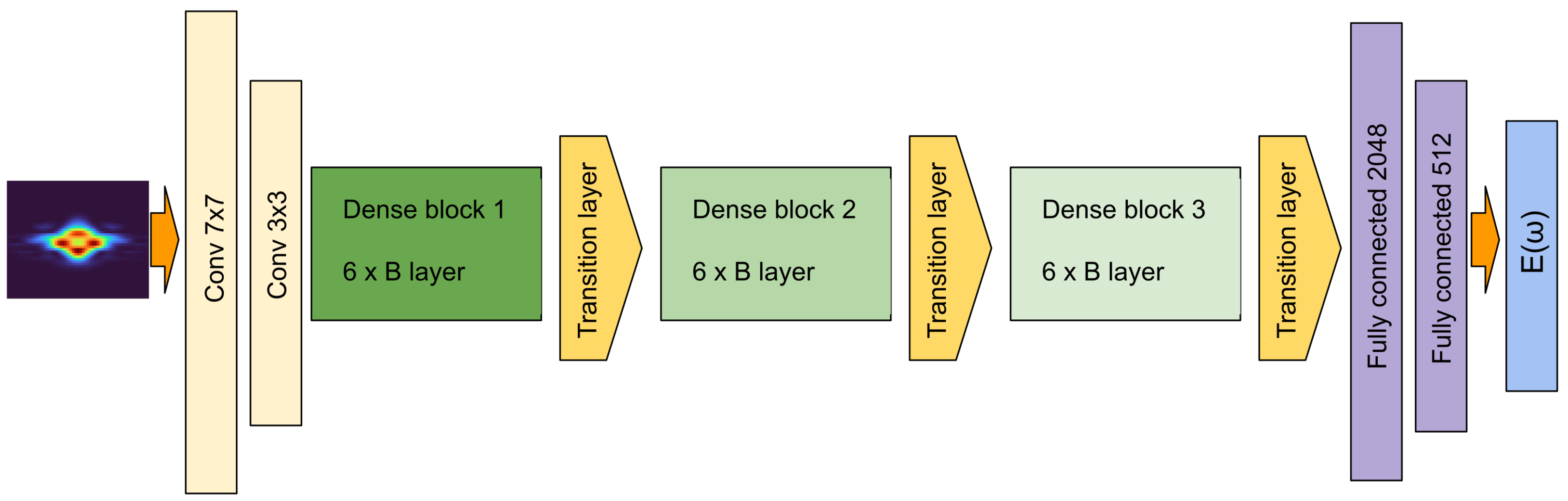
In our study, the DenseNet-BC [35,36] deep neural network was employed, being first introduced for image recognition because it showed improvements over previous neural networks like ResNet [37], GoogLeNet [38,39], FractalNets [40], or generalized ResNet [41]. DenseNet employs a dense connectivity pattern, connecting all layers with the same feature map sizes, thus ensuring a superior information and gradient flow from the input to the output layer. Feature maps are images on which some mathematical operation was performed, such as convolution. It also requires fewer trainable parameters compared to other convolutional networks. In a DenseNet-BC architecture the convolutional layers are organized in dense blocks, each of them with an equal number of layers. Inside a block the width × height size of the feature maps propagating through the block is unchanged, however the number of feature maps increases. Each layer outputs k new feature maps, and therefore the number of feature maps entering the layer is , where is the number of channels in the input layer, while k is the growth rate of the block, which doubles for subsequent dense blocks. The layers in a DenseNet-BC block are composite layers, with their main ingredient being a convolutional layer. They are designated as bottleneck layers (B in the name of the network refers to these layers), since they limit through a convolutional layer the number of input feature maps to the convolutional layers. The dense blocks are separated by transition layers that have two main features: they reduce the size of the feature maps (by applying average pooling layers) and optionally reduce the number of outgoing feature maps through convolutional layers and a compression factor c (C in the name of the network refers to this factor). The compression factor has a value between 0 and 1. In the original DenseNet paper [35], , which means that the number of input feature maps is halved at the output of the transition layer. More generally, the number of outgoing feature maps will be if the number of input feature maps to the transition layer is M.
We modified DenseNet-BC (see Figure 1) in order to fit our purpose of reconstructing ultrashort pulses. Before reaching the first dense block, the images were taken through two convolutional layers with filter sizes of and . After going through each layer the feature maps sizes are reduced by half using average pooling layers. Following that, the images reach the dense blocks section of the network, which in our case means 3 blocks separated by transition layers. Each dense block consists of 6 bottleneck layers. The first block has a growth rate of 8, which doubles for subsequent blocks. Since our images are relatively large, we also introduced a third transition layer after the last dense block to further reduce the size and number of feature maps. In the next step, the feature maps are flattened into a vector. We removed the classification layer from the original network and replaced it with two fully-connected layers with input channel sizes of 2048 and 512. The flattened vector enters these layers and the last one outputs a vector with 128 elements, consisting of the real and imaginary part of the predicted spectral electric field of the pulse. Throughout the network we use ReLU (rectified linear unit) as an activation function.
We tested several architectures for the DenseNet-BC network, however in terms of generalization, the above-described architecture proved to be adequate. Besides using the DenseNet-BC network, we built and trained our own networks. We found that even a relatively simple network with only four or five convolutional layers (with different filter sizes) and two or three fully-connected layers would lead to comparable validation errors. However, the lowest validation error and the best performance were obtained with DenseNet-BC, which is why we opted to use it in our study.
2.2. Datasets
The training of a neural network usually requires a substantial-sized dataset. Below we detail what data our dataset contains and how it is generated.
Since the training of our network follows the supervised learning methodology, we generated the actual data (the FROG images) and a label-vector, which were used to calculate the error between the CNN-predicted and the original spectral electric field. The information contained in the error function was then used to adjust the parameters of the neural network until the error reaches a minimum value and the network is optimized.
We generated our label-vectors as the spectral electric field of the ultrashort laser pulse
where the spectral phase, , is randomly generated and is unwrapped and smoothed in order to eliminate its fast variations. The spectral amplitude, , is described by a sum of Gaussian functions. The number of Gaussians is generated randomly between 10 and 30. We also randomly generated the spectral widths and the central wavelengths of the Gaussian functions. We then used to obtain the pulse in the time domain, and further on to generate the FROG spectrogram (image) according to the well-known expression for second-harmonic FROG traces [6]:
The duration of the generated pulses varies between their transform-limited duration and an upper limit of 300 fs. With this method, we generated a set of around 300,000 FROG images and the corresponding spectral electric fields.
SHG-FROG has several ambiguities. The ambiguities mean that different pulses may lead to the same FROG image, which is we have multiple label-vectors for a single FROG trace. However, multiple labels are a big problem from the perspective of training a CNN, therefore we remove these ambiguities from our data. If is the original pulse, then the following variations of the time domain would lead to the same FROG trace [6]:
- —absolute phase shift, where is the absolute phase
- —time translation by
- —time reversal
After we clean our data from ambiguities the dataset is randomly shuffled and further split into three subsets of , , and of the initial set, representing the training, the validation, and the test set. The training set is used to train the neural network while the validation set is employed for monitoring the training process for overfitting. Once the CNN is trained, we evaluate its performance on data never ‘seen’ by the CNN during training, using the test set.
2.3. Training the CNN
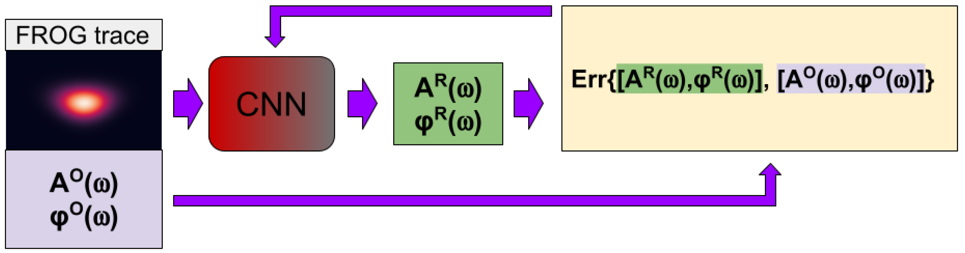
During the training of the CNN we feed the data in mini batches (batch size: 256). When a trace or a batch of traces enters the CNN they are propagated through the different layers and the final layer outputs the reconstructed spectral electric field. We used the original spectral fields, from which the traces were obtained, as labels (see Figure 2), and calculated the error between the reconstructed and original spectral fields applying the loss function, which measures the mean absolute error between the elements of the reconstructed and original vectors.
The gradient of the loss function is back-propagated through the layers of the CNN and the Adam [42] optimization algorithm updates the parameters or weights of the network according to these gradient values. Adam is a variant of the stochastic gradient descent algorithm, but implements the use of adaptive learning rates for individual parameters. The parameters are updated after the propagation of every mini-batch through the CNN until all the data in the training set are fed to the network. A single cycle of propagating the training set through the layers of the CNN is called an epoch. We trained the CNN in several hundred epochs, and the training process was monitored by calculating a validation error after every epoch. The validation error is the mean loss for the validation set, a distinct set of data, which is not used directly to train the CNN. The calculation of this error is important, since it signals if the CNN shows overfitting behavior. Overfitting refers to the over-learning of the training data and leads to poor generalization on new data. We trained our CNN on a desktop computer using the Pytorch framework as software, while the training was performed on an Nvidia GeForce 3090 Ti GPU.
3. Results and Discussion
The immediate goal of our study was to retrieve the spectral amplitude and phase of a computer-simulated ultrashort laser pulse by passing the associated FROG trace through the layers of a CNN. Although we worked with computer-simulated data, the final goal was to train a neural network capable of fast reconstruction of experimental data.
As mentioned earlier, the CNN returns the real and imaginary parts of the reconstructed spectral field. We opted for this variant instead of directly reconstructing the amplitude and the phase, since this allowed us to reconstruct the full electric field (i.e., both spectral quantities) with a single trained neural network. Moreover, given that in experiments the spectrum is usually measured, our method allows for a direct comparison between the two quantities. Finally, the real and imaginary parts of the field have significant values only in the spectral region where the spectral amplitude is significant. Using the spectral phase, which usually has large variations outside the meaningful spectral region, leads to a slower training process. Also, in time-domain the full pulse is usually described by a real quantity, with no direct access to the information regarding the phase of the pulse.
The data in the test set were used to evaluate the performance of the trained CNN. The test set contains data which are not used during the training of the neural network. It is worth mentioning that all samples in all three datasets (training, validation, and test) are entering the network as images of zero mean () and a standard deviation of one () at the pixel level. However, the CNN is trained with added Gaussian noise (, ) on the FROG traces of the training set only. The main motivation to add Gaussian noise during training is that in experimental measurements, the FROG traces may be contaminated with noise, and therefore this method is a way to improve the robustness of the reconstruction against noisy data. Nevertheless, noise may act as an augmentation method for the CNN.
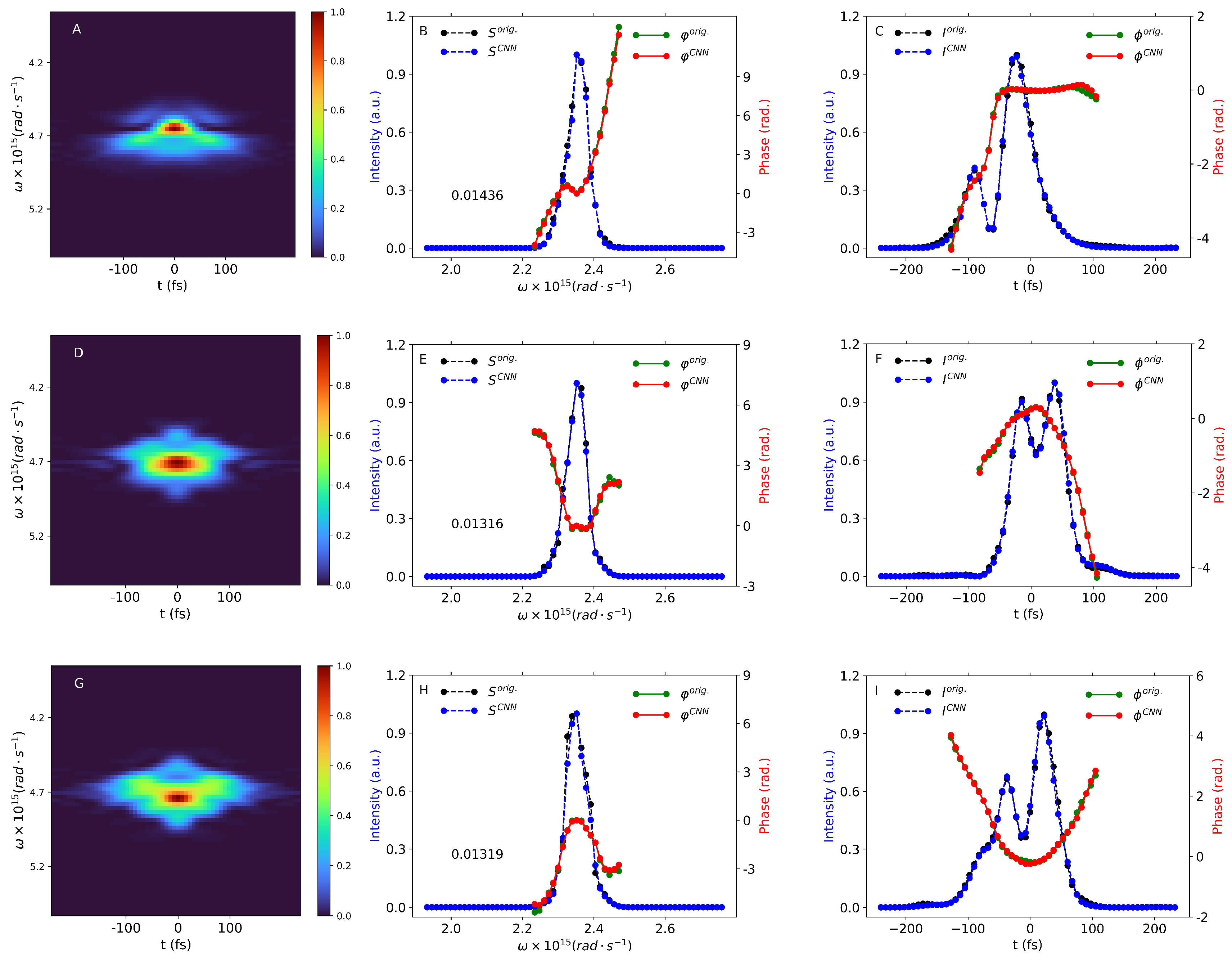
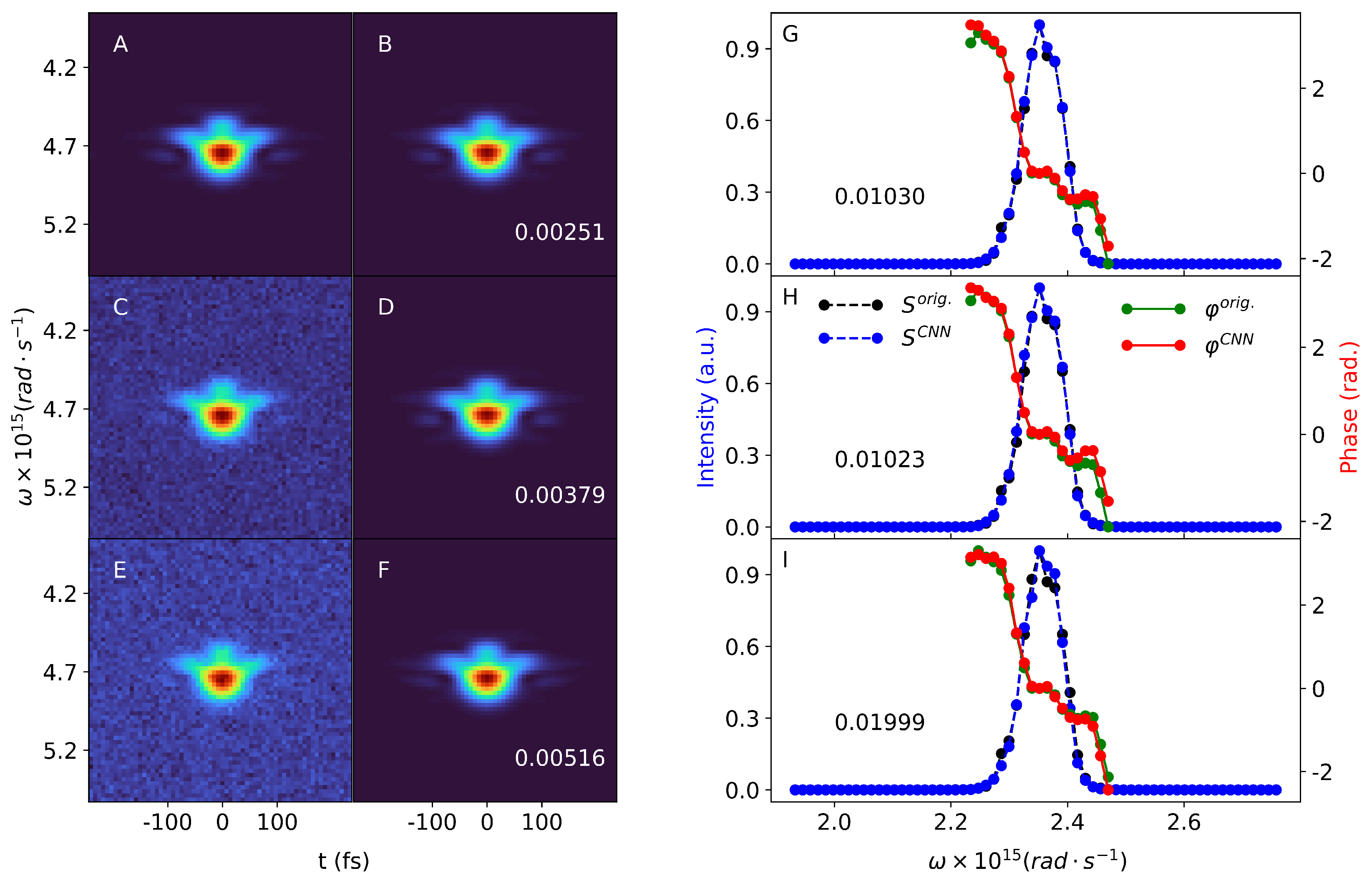
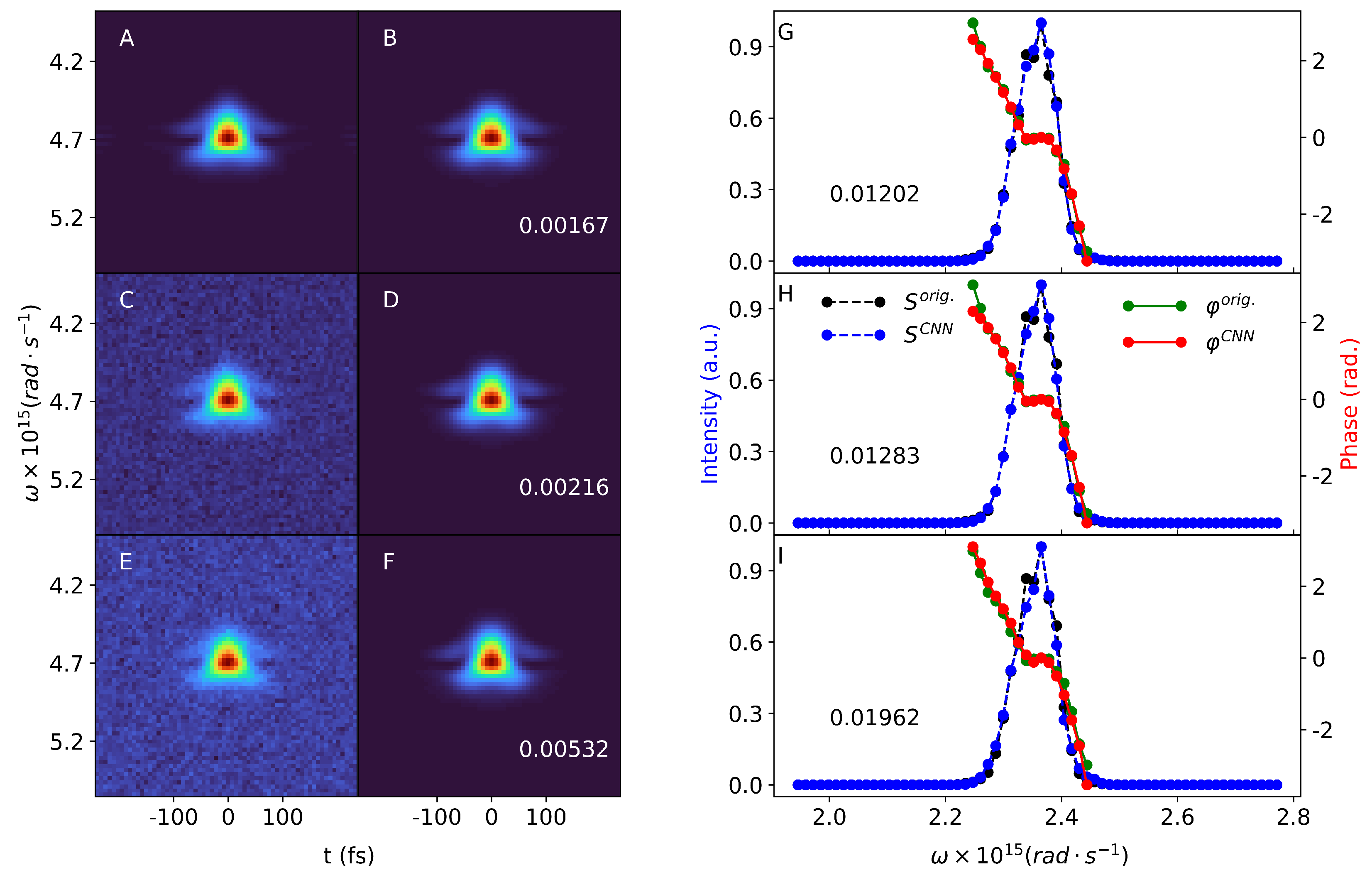
In Figure 3 we show three examples of our pulses and their reconstruction both in the spectral and time domains. In both domains, a good reconstruction of the pulse intensity and phase may be observed. These examples are taken from the test set, but may also be representative of the training and validation sets, since all these subsets were obtained by splitting a larger, randomly shuffled dataset. Our test set contains about 30,000 samples of FROG traces and the associated spectral fields. In Figure 4 and Figure 5 we show two other samples of our simulated FROG images and pulses. Here, only the spectral domain pulses are plotted, but we also show the reconstructed FROG image besides the original one. The reconstruction is performed for FROG traces, which enter the CNN with different noise levels. In these figures the first column (A, C, and E panels) contains the original FROG trace with increasing noise level from top to bottom. A: zero noise; C: Gaussian noise with and ; E: Gaussian noise with and . We mention here that the noise level on the middle FROG image has the same mean and standard deviation as the noise added during the training of the CNN. In the third column we plotted the reconstructed spectral intensities and phases corresponding to the three FROG images. Panels G, H, and I show these quantities as a function of the angular frequency . In all three cases, a good agreement between the original and the reconstructed spectral quantities was observed. This was also confirmed by the reconstruction error ( loss) calculated in every case. The error is similar for the zero noise and for the noise level with case. This is not surprising, since the latter noise level was also employed during the training of the CNN. The highest error value was found for the highest noise level. For a single FROG trace, the reconstruction time is on the millisecond scale (about 30 ms) on a GHz computer. We also calculated the mean loss for the entire test set, which are , , and for increasing noise levels. Our simulated pulse from Figure 4 was also reconstructed with the FROG code [43] of the Trebino group, and the comparison with the CNN is summarized in the table below. We tested the reconstruction without and with noise ( = 0.15), but without any pre-processing of the noisy traces. Table 1 shows that the CNN time and error does not noticeably change, while reconstruction with the FROG code takes a longer time period for the same or even higher errors.
The reconstructed spectral intensity and phase were used to reconstruct the FROG trace itself for all noise levels mentioned above. The reconstructed FROG traces are plotted in the second column of Figure 4 and Figure 5 (panels B, D, and F), along with the reconstruction error [6] G, for FROG traces, where:
Here, N is the size of the FROG image in pixels, while and are the original FROG with zero noise and the reconstructed FROG trace, respectively. As shown in the second column of Figure 4 and Figure 5, the reconstructed FROG traces are very similar to the original ones. The G reconstruction error is lowest for the zero noise case, while the highest reconstruction error is found again for the highest noise level added to the FROG images.
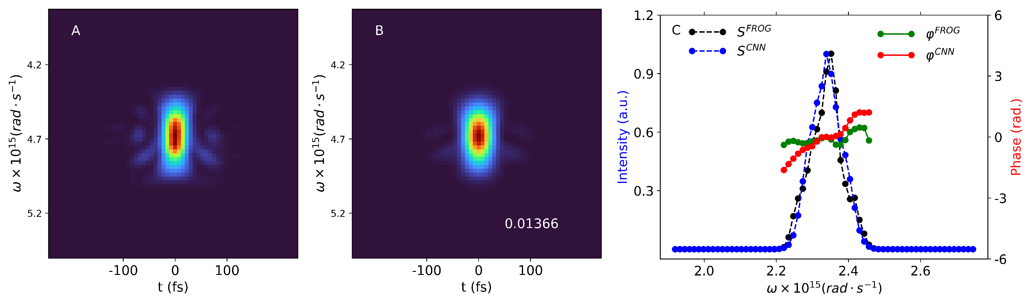
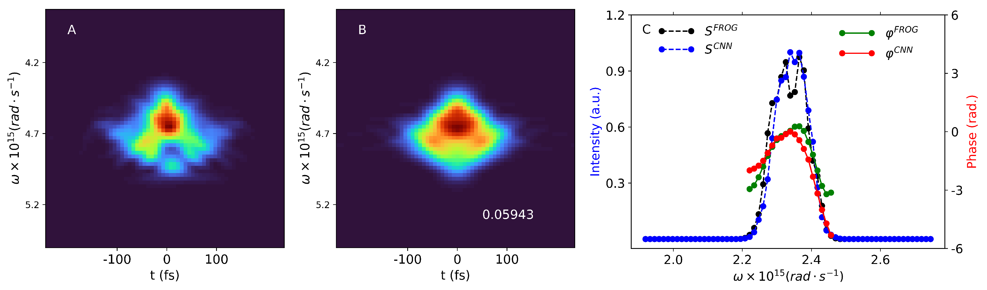
We tested our trained CNN on two experimentally measured SHG-FROG traces, shown in Figure 6 and Figure 7 (panel A). The experimental FROG traces of laser pulses centered around 800 nm were measured with grating-eliminated no-nonsense observation of ultrafast incident laser light E fields (GRENOUILLE) [44] at CoRELS. The grid size of the measured FROG traces was 64 with a delay increment of fs. In the third panel (C) of Figure 6 and Figure 7 we plotted the retrieved spectral intensity and phase, where we compared the results of two different reconstruction algorithms: the GRENOUILLE’s built-in algorithm and our CNN method. The general trend of the curves agrees for both retrieval methods and spectral quantities. More specifically, the spectral phases overlap along a certain frequency range, where the intensity has significant values. For both pulses the spectral intensities show similar shapes for both retrieval algorithms; in the case of the second pulse the CNN can even resolve the two-peak structure of the intensity. However, there are also obvious discrepancies between the curves retrieved by GRENOUILLE’s built-in algorithm and our CNN. According to the GRENOUILLE’s software, the FWHM duration of the first pulse is fs, while our method gives a FWHM duration of 30 fs. For the second experimental pulse the estimated durations were fs and 75 fs, respectively. This can be roughly observed on the original and reconstructed frog traces, where at the central frequency the red portion of the spectrograms has approximately the same width along the temporal axis on Figure 6, while on Figure 7 this is larger in the case of the reconstructed trace.
Panel B on both Figure 6 and Figure 7 show our retrieved FROG spectrograms. Again, one may observe good similarities between the retrieved and the experimental FROG traces: for example, our method nicely reproduces some of the ‘wings’ observed in the experimental FROG in Figure 6. The G FROG errors between the experimental and our CNN retrieved FROG trace are and for the experimental pulses in Figure 6 and Figure 7, respectively. The same errors in case of GRENOUILLE’s built-in software are and , respectively. Although these values are slightly lower than in the case of the CNN reconstruction, we emphasize that our method relies only on simulated data, while the FROG algorithm used by the GRENOUILLE setup uses input from the experimentally measured traces. Given that the CNN was trained only with these computer generated FROG traces, this is a remarkable performance, and in the same time a very fast pulse reconstruction process. Also, our method does not need any background noise subtraction compared to the GRENOUILLE software, which may constitute a further speed boost.
4. Conclusions
We developed a CNN-based method in order to retrieve the spectral intensity and phase of ultrashort laser pulses from simulated SHG-FROG traces. The neural network was trained with computer-simulated FROG traces and the corresponding spectral domain pulses employed as labels. The performance of the CNN was tested on a set of about 30,000 FROG samples, which were not employed during the training of the network. We found an excellent performance in retrieving the spectral intensity and phase of simulated pulses with very low pulse reconstruction errors ( loss) and FROG errors G.
One of the main advantages of our method is a very fast reconstruction of ultrashort laser pulses. The CNN reconstructs a single pulse on the millisecond scale, while classical, iterative algorithms usually provide reliable results on a longer timescale. The speed of the reconstruction is especially useful for tuning and adjusting the high repetition rate laser systems in real time. Also, our method does not need any background noise substraction, unlike, for example, the GRENOUILEE software, which automatically substracts any unwanted background noise. As shown above for simulated pulses, the CNN is very robust to noisy data. Another advantage is that the CNN is trained to reconstruct the complex spectral electric field, which provides both the spectral intensity and phase using a single trained neural network. This method also makes a direct comparison possible with measured spectral intensities. Further, the reconstructed complex spectral field gives direct access to the spectral phase. In time-domain, for pulses described by real fields the phase information would not be directly accessible.
As mentioned earlier, our goal was to reconstruct simulated ultrashort pulses. However, we wanted to further test our method, therefore we reconstructed two experimentally measured FROG traces. The CNN retrieved spectral intensity and phase was compared to the corresponding quantities retrieved by the built-in software of the GRENOUILLE setup, which measured the experimental pulses. Trained only on simulated pulses, the CNN was able to qualitatively reproduce the experimental pulses, providing relatively low FROG reconstruction errors and comparable pulse durations compared to the FROG software. Although the FROG errors provided by the GRENOUILLE software are slightly lower, we emphasize again that our method relies only on simulated data, while the FROG algorithm used by the GRENOUILLE setup uses input from the experimentally measured traces. Nevertheless, further improvements need to be implemented in order to achieve a better performance. We plan to combine this method with a semi-empirical spectral phase generation method. The latter is based on the Taylor expansion of the spectral phase, where the expansion coefficients of the second and higher order terms are calculated taking into account several parameters of the pulse compressor, like the incident angle or the grating distance. Transfer learning between the two methods would also be worth exploring. Obviously, a larger and more diverse dataset would potentially add further improvements to the performance of the network.
Author Contributions
Conceptualization K.K. and V.T.; methodology and software I.T. and V.T.; validation I.T., A.M.M.G., K.K. and V.T.; experimental measurements W.C. and H.Y.; writing—original draft preparation I.T.; writing—review and editing I.T., V.T., A.M.M.G. and K.K.; visualization I.T. All authors have read and agreed to the published version of the manuscript.
Funding
This research was funded by a grant of the Romanian National Authority for Scientific Research, CNCS-UEFISCDI, project PN-III-P5-ELI-RO, project number ELI_03/01.10.2020 and by the Ministry of Research, Innovation and Digitalisation through Programme 1—Development of the National Research and Development System, Subprogramme 1.2—Institutional Performance—Funding Projects for Excellence in RDI, Contract No. 37PFE/30.12.2021.
Institutional Review Board Statement
Not applicable.
Informed Consent Statement
Not applicable.
Data Availability Statement
Data available on request.
Conflicts of Interest
The authors declare no conflict of interest.
Abbreviations
The following abbreviations are used in this manuscript:
| FROG | Frequency Resolved Optical Gating |
| SHG-FROG | Second-Harmonics Generation Frequency Resolved Optical Gating |
| RABBITT | reconstruction of attosecond beating by interference of two-photon transitions |
| SPIDER | spectral phase interferometry for direct electric-field reconstruction of ultrashort |
| optical pulses | |
| TIPTOE | tunneling ionization with a perturbation for the time-domain observation of |
| an electric field | |
| CNNs | Convolutional Neural Networks |
| GRENOUILLE | Grating-eliminated no-nonsense observation of ultrafast incident laser light |
| E fields |
References
- Brabec, T.; Krausz, F. Intense few-cycle laser fields: Frontiers of nonlinear optics. Rev. Mod. Phys. 2000, 72, 545. [Google Scholar] [CrossRef]
- Liang, J.; Wang, L.V. Single-shot ultrafast optical imaging. Optica 2018, 5, 1113–1127. [Google Scholar] [CrossRef] [PubMed]
- Zhao, J.; Li, M. Lensless ultrafast optical imaging. Light Sci. Appl. 2022, 11, 97. [Google Scholar] [CrossRef]
- Peng, P.; Marceau, C.; Villeneuve, D.M. Attosecond imaging of molecules using high harmonic spectroscopy. Nat. Rev. Phys. 2019, 1, 144–155. [Google Scholar] [CrossRef]
- Schreiber, J.; Bolton, P.R.; Parodi, K. “Hands-on” laser-driven ion acceleration: A primer for laser-driven source development and potential applications. Rev. Sci. Instrum. 2016, 87, 071101. [Google Scholar] [CrossRef] [PubMed]
- Trebino, R. Frequency Resolved Optical Gating: The Measurment of Ultrashort Laser Pulses; Springer Science: Berlin/Heidelberg, Germany, 2000. [Google Scholar]
- Trebino, R.; DeLong, K.W.; Fittinghoff, D.N.; Sweetser, J.N.; Krumbügel, M.A.; Richman, B.A.; Kane, D.J. Measuring ultrashort laser pulses in the time-frequency domain using frequency-resolved optical gating. Rev. Sci. Instrum. 1997, 68, 3277–3295. [Google Scholar] [CrossRef]
- Paul, P.M.; Toma, E.S.; P. Breger, G.M.; Auge, F.; Balcou, P.; Muller, H.G.; Agostini, P. Observation of a train of attosecond pulses from high harmonic generation. Science 2001, 292, 1689–1692. [Google Scholar] [CrossRef]
- Muller, H. Reconstruction of attosecond harmonic beating by interference of two-photon transitions. Appl. Phys. B 2002, 74 (Suppl. 1), s17–s21. [Google Scholar] [CrossRef]
- Iaconis, C.; Walmsley, I.A. Spectral phase interferometry for direct electric-field reconstruction of ultrashort optical pulses. Opt. Lett. 1998, 23, 792–794. [Google Scholar] [CrossRef]
- Park, S.B.; Kim, K.; Cho, W.; Hwang, S.I.; Ivanov, I.; Nam, C.H.; Kim, K.T. Direct sampling of a light wave in air. Optica 2018, 5, 402–408. [Google Scholar] [CrossRef]
- Miranda, M.; Fordell, T.; Arnold, C.; L’Huillier, A.; Crespo, H. Simultaneous compression and characterization of ultrashort laser pulses using chirped mirrors and glass wedges. Opt. Express 2012, 20, 688–697. [Google Scholar] [CrossRef] [PubMed]
- Xu, B.; Gunn, J.M.; Cruz, J.M.D.; Lozovoy, V.V.; Dantus, M. Quantitative investigation of the multiphoton intrapulse interference phase scan method for simultaneous phase measurement and compensation of femtosecond laser pulses. J. Opt. Soc. Am. B 2006, 23, 750–759. [Google Scholar] [CrossRef]
- Anashkina, E.A.; Ginzburg, V.N.; Kochetkov, A.A.; Yakovlev, I.V.; Kim, A.V.; Khazanov, E.A. Single-shot laser pulse reconstruction based on self-phase modulated spectra measurements. Sci. Rep. 2016, 6, 33749. [Google Scholar] [CrossRef] [PubMed]
- Amat-Roldán, I.; Cormack, I.G.; Loza-Alvarez, P.; Artigas, D. Measurement of electric field by interferometric spectral trace observation. Opt. Lett. 2005, 30, 1063–1065. [Google Scholar] [CrossRef]
- Yang, S.D.; Hsu, C.S.; Lin, S.L.; Miao, H.; Huang, C.B.; Weiner, A.M. Direct spectral phase retrieval of ultrashort pulses by double modified one-dimensional autocorrelation traces. Opt. Express 2008, 16, 20617–20625. [Google Scholar] [CrossRef]
- Kane, D.J. Principal components generalized projections: A review [Invited]. J. Opt. Soc. Am. B 2008, 25, A120–A132. [Google Scholar] [CrossRef]
- Sidorenko, P.; Lahav, O.; Avnat, Z.; Cohen, O. Ptychographic reconstruction algorithm for frequency-resolved optical gating: Super-resolution and supreme robustness. Optica 2016, 3, 1320–1330. [Google Scholar] [CrossRef]
- Escoto, E.; Tajalli, A.; Nagy, T.; Steinmeyer, G. Advanced phase retrieval for dispersion scan: A comparative study. J. Opt. Soc. Am. B 2018, 35, 8–19. [Google Scholar] [CrossRef]
- Fittinghoff, D.N.; DeLong, K.W.; Trebino, R.; Ladera, C.L. Noise sensitivity in frequency-resolved optical-gating measurements of ultrashort pulses. J. Opt. Soc. Am. B 1995, 12, 1955–1967. [Google Scholar] [CrossRef]
- Xu, L.; Zeek, E.; Trebino, R. Simulations of frequency-resolved optical gating for measuring very complex pulses. J. Opt. Soc. Am. B 2008, 25, A70–A80. [Google Scholar] [CrossRef]
- Goodfellow, I.; Bengio, Y.; Courville, A. Deep Learning; The MIT Press: Cambridge, MA, USA, 2016. [Google Scholar]
- Krizhevsky, A.; Sutskever, I.; Hinton, G.E. ImageNet Classification with Deep Convolutional Neural Networks. In Advances in Neural Information Processing Systems; Pereira, F., Burges, C., Bottou, L., Weinberger, K., Eds.; Curran Associates, Inc.: Red Hook, NY, USA, 2012; Volume 25. [Google Scholar]
- Esteva, A.; Kuprel, B.; Novoa, R.A.; Ko, J.; Swetter, S.M.; Blau, H.M.; Thrun, S. Dermatologist-level classification of skin cancer with deep neural networks. Nature 2017, 542, 115–118. [Google Scholar] [CrossRef] [PubMed]
- Reichstein, M.; Camps-Valls, G.; Stevens, B.; Jung, M.; Denzler, J.; Carvalhais, N.; Prabhat. Deep learning and process understanding for data-driven Earth system science. Nature 2019, 566, 195–204. [Google Scholar] [CrossRef] [PubMed]
- Wu, H.; Zhou, H.; Long, M.; Wang, J. Interpretable weather forecasting for worldwide stations with a unified deep model. Nat. Mach. Intell. 2023, 5, 602–611. [Google Scholar] [CrossRef]
- Raissi, M.; Perdikaris, P.; Karniadakis, G. Physics-informed neural networks: A deep learning framework for solving forward and inverse problems involving nonlinear partial differential equations. J. Comput. Phys. 2019, 378, 686–707. [Google Scholar] [CrossRef]
- Karniadakis, G.E.; Kevrekidis, I.G.; Lu, L.; Perdikaris, P.; Wang, S.; Yang, L. Physics-informed machine learning. Nat. Rev. Phys. 2021, 3, 422–440. [Google Scholar] [CrossRef]
- Kazemzadeh, M.; Hisey, C.L.; Zargar-Shoshtari, K.; Xu, W.; Broderick, N.G. Deep convolutional neural networks as a unified solution for Raman spectroscopy-based classification in biomedical applications. Opt. Commun. 2022, 510, 127977. [Google Scholar] [CrossRef]
- Gherman, A.M.M.; Kovács, K.; Cristea, M.V.; Toșa, V. Artificial Neural Network Trained to Predict High-Harmonic Flux. Appl. Sci. 2018, 8, 2106. [Google Scholar] [CrossRef]
- Queen, O.; McCarver, G.A.; Thatigotla, S.; Abolins, B.P.; Brown, C.L.; Maroulas, V.; Vogiatzis, K.D. Polymer graph neural networks for multitask property learning. npj Comput. Mater. 2023, 9, 90. [Google Scholar] [CrossRef]
- Krumbügel, M.A.; Ladera, C.L.; DeLong, K.W.; Fittinghoff, D.N.; Sweetser, J.N.; Trebino, R. Direct ultrashort-pulse intensity and phase retrieval by frequency-resolved optical gating and a computational neural network. Opt. Lett. 1996, 21, 143–145. [Google Scholar] [CrossRef]
- Zahavy, T.; Dikopoltsev, A.; Moss, D.; Haham, G.I.; Cohen, O.; Mannor, S.; Segev, M. Deep learning reconstruction of ultrashort pulses. Optica 2018, 5, 666. [Google Scholar] [CrossRef]
- Kleinert, S.; Tajalli, A.; Nagy, T.; Morgner, U. Rapid phase retrieval of ultrashort pulses from dispersion scan traces using deep neural networks. Opt. Lett. 2019, 44, 979–982. [Google Scholar] [CrossRef] [PubMed]
- Huang, G.; Liu, Z.; Van Der Maaten, L.; Weinberger, K.Q. Densely Connected Convolutional Networks. In Proceedings of the 2017 IEEE Conference on Computer Vision and Pattern Recognition (CVPR), Honolulu, HI, USA, 21–26 July 2017; pp. 2261–2269. [Google Scholar] [CrossRef]
- Amos, B.; Kolter, J.Z. A PyTorch Implementation of DenseNet. Available online: https://github.com/bamos/densenet.pytorch (accessed on 1 October 2021).
- He, K.; Zhang, X.; Ren, S.; Sun, J. Deep Residual Learning for Image Recognition. In Proceedings of the 2016 IEEE Conference on Computer Vision and Pattern Recognition (CVPR), Las Vegas, NV, USA, 27–30 June 2016; pp. 770–778. [Google Scholar] [CrossRef]
- Szegedy, C.; Liu, W.; Jia, Y.; Sermanet, P.; Reed, S.; Anguelov, D.; Erhan, D.; Vanhoucke, V.; Rabinovich, A. Going deeper with convolutions. In Proceedings of the 2015 IEEE Conference on Computer Vision and Pattern Recognition (CVPR), Boston, MA, USA, 7–12 June 2015; pp. 1–9. [Google Scholar] [CrossRef]
- Szegedy, C.; Vanhoucke, V.; Ioffe, S.; Shlens, J.; Wojna, Z. Rethinking the Inception Architecture for Computer Vision. In Proceedings of the 2016 IEEE Conference on Computer Vision and Pattern Recognition (CVPR), Las Vegas, NV, USA, 27–30 June 2016; pp. 2818–2826. [Google Scholar] [CrossRef]
- Larsson, G.; Maire, M.; Shakhnarovich, G. Fractalnet:Ultra-deep neural networks without residuals. arXiv 2016, arXiv:1605.07648. [Google Scholar]
- Targ, S.; Almeida, D.; Lyman, K. Resnet in Resnet: Generalizing Residual Architectures. arXiv 2016, arXiv:1603.08029. [Google Scholar]
- Kingma, D.P.; Ba, J. Adam: A Method for Stochastic Optimization. arXiv 2015, arXiv:1412.6980. [Google Scholar]
- Code for Retrieving a Pulse Intensity and Phase from Its FROG Trace, Prof. Rick Trebino: Ultrafast Optics Group. Available online: https://frog.gatech.edu/code.html (accessed on 16 October 2023).
- O’shea, P.; Kimmel, M.; Gu, X.; Trebino, R. Highly simplified device for ultrashort-pulse measurement. Opt. Lett. 2001, 26, 932–934. [Google Scholar] [CrossRef]
Figure 1.
Schematics for the modified DenseNet-BC neural network. Details about the network are described in the text.
Figure 1.
Schematics for the modified DenseNet-BC neural network. Details about the network are described in the text.

Figure 2.
Schematics for the training process of the convolutional neural network. After the FROG traces are propagated through the layers of the CNN, the network outputs a reconstructed (R) spectral field, characterized by the spectral amplitude and phase, and . The loss is then calculated between the reconstructed and the original (O) spectral fields. The gradient of the loss function is then back-propagated and the parameters of the CNN are adjusted accordingly.

Figure 3.
Reconstruction of three simulated pulses in the spectral and temporal domain. Each row contains the original FROG image, the original and reconstructed spectral intensity (S) and phase () and the temporal intensity (I) and phase (). Panels (A–C): first pulse. Panels (D–F): second pulse. Panels (G–I): third pulse. In the spectral domain the (Equation (3)) reconstruction error is also shown on the figures.

Figure 4.
Reconstruction of a computer-simulated pulse. Panels (A,C,E): original FROG traces with different noise levels, as detailed in the text. Panels (B,D,F): reconstructed FROG traces showing the FROG reconstruction error defined in Equation (4). The FROG traces are normalized to one (dark red color). Also, the color code is the same as in Figure 3. Panels (G–I): black dashed line with circles: original intensity; blue dashed line with circles: CNN-retrieved intensity; green line with circles: original spectral phase; Red line with circles: CNN reconstructed spectral phase. Panels (G–I) also show the (Equation (3)) reconstruction error for the pulses, as detailed in the text.

Figure 5.
Reconstruction of a second computer-simulated pulse. Panels (A,C,E): original FROG traces with different noise levels, as detailed in the text. Panels (B,D,F): reconstructed FROG traces showing the FROG reconstruction error defined in Equation (4). The FROG traces are normalized to one (dark red color). Also, the color code is the same as in Figure 3. Panels (G–I): black dashed line with circles: original intensity; blue dashed line with circles: CNN retrieved intensity; green line with circles: original spectral phase; Red line with circles: CNN reconstructed spectral phase. Panels (G–I) also show the (Equation (3)) reconstruction error for the pulses, as detailed in the text.

Figure 6.
Reconstruction of an experimental ultrashort laser pulse. Panel (A): experimental FROG trace. Panel (B): retrieved FROG trace showing the FROG reconstruction error defined in Equation (4). The FROG traces are normalized to one (dark red color). Also, the color code is the same as in Figure 3. Panel (C): black dashed line with circles: intensity retrieved by GRENOUILLE’s built-in algorithm; blue dashed line with circles: CNN retrieved intensity; green line with circles: spectral phase retrieved by GRENOUILLE’s built-in algorithm; red line with circles: CNN reconstructed spectral phase.

Figure 7.
Reconstruction of a second experimental ultrashort laser pulse. Panel (A): experimental FROG trace. Panel (B): retrieved FROG trace showing the FROG reconstruction error defined in Equation (4). The FROG traces are normalized to one (dark red color). Also the color code is the same as in Figure 3. Panel (C): black dashed line with circles: intensity retrieved by GRENOUILLE’s built-in algorithm; blue dashed line with circles: CNN retrieved intensity; green line with circles: spectral phase retrieved by GRENOUILLE’s built-in algorithm; red line with circles: CNN-reconstructed spectral phase.


Disclaimer/Publisher’s Note: The statements, opinions and data contained in all publications are solely those of the individual author(s) and contributor(s) and not of MDPI and/or the editor(s). MDPI and/or the editor(s) disclaim responsibility for any injury to people or property resulting from any ideas, methods, instructions or products referred to in the content. |
© 2023 by the authors. Licensee MDPI, Basel, Switzerland. This article is an open access article distributed under the terms and conditions of the Creative Commons Attribution (CC BY) license (https://creativecommons.org/licenses/by/4.0/).
Share and Cite
MDPI and ACS Style
Tóth, I.; Gherman, A.M.M.; Kovács, K.; Cho, W.; Yun, H.; Toşa, V. Reconstruction of Femtosecond Laser Pulses from FROG Traces by Convolutional Neural Networks. Photonics 2023, 10, 1195. https://doi.org/10.3390/photonics10111195
AMA Style
Tóth I, Gherman AMM, Kovács K, Cho W, Yun H, Toşa V. Reconstruction of Femtosecond Laser Pulses from FROG Traces by Convolutional Neural Networks. Photonics. 2023; 10(11):1195. https://doi.org/10.3390/photonics10111195
Chicago/Turabian StyleTóth, István, Ana Maria Mihaela Gherman, Katalin Kovács, Wosik Cho, Hyeok Yun, and Valer Toşa. 2023. "Reconstruction of Femtosecond Laser Pulses from FROG Traces by Convolutional Neural Networks" Photonics 10, no. 11: 1195. https://doi.org/10.3390/photonics10111195
Note that from the first issue of 2016, this journal uses article numbers instead of page numbers. See further details here.