
A Simple Nozzle-Diffuser Duct Used as a Kuroshio Energy Harvester
by
 ,
,
Po-Hung Yeh
1 ,
,
Shang-Yu Tsai
1,
Wei-Ren Chen
1,
Shing-Nan Wu
1,
Meng-Chang Hsieh
2 and
Bang-Fuh Chen
1,* 1
Department of Marine Environment and Engineering, National Sun Yat-sen University, Kaohsiung 80424, Taiwan
2
Institute of Undersea Technology, National Sun Yat-sen University, Kaohsiung 80424, Taiwan
*
Author to whom correspondence should be addressed.
Processes 2021, 9(9), 1552; https://doi.org/10.3390/pr9091552
Submission received: 19 July 2021
/
Revised: 18 August 2021
/
Accepted: 26 August 2021
/
Published: 30 August 2021
(This article belongs to the Section Energy Systems)
Abstract
:In response to the increasing energy demand in Taiwan and the global trend of renewable energy development, Kuroshio energy is a potential energy source. How to extract this invaluable natural resource has then become an intriguing and important question in engineering practices. This study reported the results of a feasibility study for a nozzle-diffuser duct (NDD) as the Kuroshio currents energy harvester. The computational fluid dynamics (CFD) software ANSYS Fluent was employed to calculate the drag and added mass coefficients of the duct anchored to the seabed. Those coefficients were further imported into Orcaflex to simulate the motion of the duct under normal and storm wave conditions. Results showed that the duct was stable 25 m below the sea surface under normal wave conditions. When the wave condition changed to storm waves, the duct needed to dive into at least 90 m below the sea surface to regain its stability and obtain high power take-off (PTO). An optimal design nozzle-diffuser-duct was reported, and a PTO peak of 15 kW was expectable in the Kuroshio currents. Once a suitable offshore platform can be developed with sixty-six NDDs, a Megawatt Kuroshio ocean current power generation system is feasible in the near future.
1. Introduction
Even though the electrical energy demand in the world keeps increasing in most countries, primary electricity generation is still from non-renewable fuels like coal, natural gas, nuclear, and petroleum. However, burning fossil fuels is harmful to the environment, and fuel supply is usually limited and subject to price volatility. Nuclear power, a low-carbon power generation method, also poses sharp threats to human beings and the environment. Disposal of nuclear waste, potential radioactive contamination by accidents and sabotage, and the threat of nuclear proliferation are merely three of many unresolved controversies that prevent using nuclear power to generate electricity for civilian purposes. In contrast, green energies, such as solar, wind, and ocean powers, are indigenous, non-polluting, and inexhaustible. After being developed for decades, the technologies for both solar and wind power generation are mature. However, the development of ocean current power generation is still under headwind.
Taiwan relies on importing most of its energy resources to ensure long-term sustainability and energy supply security; diversifying energy supply to renewable energy is a national energy strategy for Taiwan. Among the three aforementioned renewable energy technologies, the potential of wind power generation in Taiwan is the highest. The average wind speed of the northeast monsoon usually exceeds 4 m/s, making many coastal and offshore areas in Taiwan quite abundant in wind energy. As of 2018, the capacity of wind power in Taiwan was 704 MW [1]. The Taiwanese government also aims to increase the capacity of offshore wind power to 5.5 GW by 2025, according to the Ministry of Economic Affairs (MOEA). However, the available wind speed to generate power is largely affected by the variation of weather. While most of the available wind speed occurs during the wintertime, high energy use usually happens in summer when the wind speed is relatively low. Due to this seasonal non-uniformity, although the capacity factor of wind power could obtain as high as 70% in the wintertime, only 6% can be achieved in the summer season [2]. It has hampered wind power from becoming a reliable energy supply in Taiwan. On the other hand, ocean energy has the advantage of becoming a good alternative energy source. It includes both the wave power generated by surface waves and tidal power created by the moving water driven by tides. These two kinds of power can be harvested and transformed into electricity, and thus have the potential to provide a substantial amount of renewable energy. It is expected to fulfill the gap that the share of renewable energy should reach 20% by 2025. Taiwan is an island situated in the western Pacific Ocean, and a strong ocean current flow past Taiwan all the time. Seasonal non-uniformity of weather and shortage of land resources are no longer the essential issues to obstacle its development. Thus, whether the technology is able to capture the energy successfully and the power generation system can survive in the violent marine environment have become the most critical and relevant challenges for the island nation to reach its goal.
1.1. Kuroshio Current
As shown in Figure 1, the Kuroshio currents are strong ocean currents flowing northerly on the western North Pacific Ocean, comprising the western boundary of the North Pacific Subtropical Gyre (NPSG). It originates from the westward flowing North Equatorial Current (NEC) at the east coast of Luzon, Philippines, flows northerly past the east coast of Taiwan and Japan, and eventually merges into the eastward flowing North Pacific Current (NPC). Analogous to the Gulf Stream in the Atlantic Ocean, the Kuroshio transports a large amount of heat and warm water from the tropics towards the polar region. Its speed is about 0.5–2.0 m/s, and the current has a volume transport measured at about 20–40 × 106 m3/s which is about 100 times more than the Amazon River [3]. Compared to wind power generation, which needs the wind speed to reach at least 9.0 m/s for a good wind farm, ocean current only has to obtain one-tenth of the speed to generate the same amount of power because of the density difference between the air and seawater. Besides, wind turbines are not able to work twenty-four hours per day since the appropriate wind speed is not always available. Ocean current, such as the Kuroshio current, is stable in flow with little fluctuation regardless of time. An efficient generator converting power of the ocean current may be functioning for more than three hundred days in a year [3]. As such, the massive power of the Kuroshio current will constitute a stable power source.
1.2. Development for Ocean Current Energy Harvester
Three teams from three different universities in Taiwan, National Taiwan University (NTU), National Sun Yat-sen University (NSYSU), and National Taiwan Ocean University (NTOU), had made progress in conducting preliminary studies on power harvesting from the Kuroshio current. The Floating Kuroshio Turbine (FKT) system (Figure 2) was the collaboration by NTU and NTOU [4]. A laboratory flume test demonstrated that a 1/25 model could generate 850 W of power when the model was towed at a speed of 1.45 m/s [5]. A feasibility study for a 1/5 model has been conducted; it is expected that the larger model would generate higher power up to 20 kW. The team from NSYSU designed a floating nozzle-diffusor duct (NDD) power generation system (Figure 3a) and deployed it successfully in the sea area near the Penghu cross-sea bridge in 2013 (Figure 3b). The in-situ test for the power take-off (PTO) of the system reached as high as 5 kW [6]. A successive new design with a circular nozzle-diffusor duct is expected to increase the PTO three times more than the previous model [7]. Another team from NSYSU, cooperating with THL (Tainan Hydraulics Laboratory) and Wanchi Steel Industry Company, developed a 50 kW Kuroshio ocean current power-energy harvester [8]. During the 60-h open-water towing test in southeast Taiwan in 2016, an average of 26 kW of power was reported under the current speed of 1.27 m/s.
Besides the aforementioned developments in Taiwan, Japan’s New Energy and Industrial Technology Development Organization (NEDO), together with IHI Corporation and Toshiba Corporation have been developing a next-generation ocean energy power generation, the so-called underwater floating type ocean current turbine system. The underwater floating “Kairyu” is a 100 kW power generation system with two 50 kW counter-rotating turbines of 11-m blades. The Kairyu system consists of floating generator sets moored underwater, each of which is approximately 20 m in length and width. It generates electricity through a turbine with a diameter of 11 m, which revolves around ocean currents as an energy source. Two turbines with counter-rotating blades cancel each other’s torque, so the unit can maintain its stable position and generate electricity efficiently [9]. In addition, Swedish developer Minesto designed the tidal power generating kite “Deep Green” anchored to the seabed and “flying” underwater [10]. It was designed specifically to work in the marine environment with slow current speed. A demonstrator has been installed off the coast of Northern Ireland and generating electricity for more than two years. In 2018, a commercial scale (500 kW) Deep Green was commissioned at the site off the coast of North Wales. Recently, enormous related studies were reported, such as [11,12,13,14,15], among many others. A brief literature review for the development of ocean current energy harvester can be found in [6].
This study’s objective was to attempt to carry out a feasibility study for the employment of an energy harvester (nozzle-diffusor duct, NDD) [7,16] in the marine environment of Kuroshio currents. Utilizing ANSYS Fluent, an acceleration method was developed to estimate the drag and add mass coefficients for the 6DoF motions of the NDD. These coefficients were further used in OrcaFlex to calculate the hydrodynamic forces exerted on a single duct anchored to the seabed. Dynamic simulations under normal and storm wave conditions were then performed to investigate the corresponding responses of the system. Adequate submerged depth of the duct to avoid large storm waves and have high power take-off at the same time was discussed. Finally, suggestions for a sparing system to carry plural ducts and some concluding remarks drawn from this study were addressed.
2. Numerical Method
Commercial CFD code ANSYS Fluent was used to conduct numerical simulations. The fluid was assumed incompressible with constant density and molecular viscosity. The governing equations of continuity and Reynolds-averaged Navier-Stokes (RANS) equations for the flow mean quantities are:
where is the Reynolds stress tensor and the main reason for the closure problem in turbulence. ANSYS Fluent provides several different RANS models to solve the closure problem, e.g., Standard k-ε, RNG k-ε, Realizable k-ε, Standard k-ω, SST k-ω, and Reynolds stress model. Considering the robustness of accuracy and its ability for rapid prediction, this study used the Realizable k-ε model, which provided better performance compared with the Standard k-ε model for flows involving rotation, adverse pressure gradient, and separation.
2.1. Domain and Convergence Tests
In this study, a nozzle-diffusor duct (NDD) designed by [16] was used as the device to capture ocean current energy. Figure 4 shows the 3D diagram and plan view of the NDD used in the simulations. To avoid large mesh deformation near the NDD surface, the smaller grid size surrounding the duct was used. Different initial mesh sizes, mesh size growth rate, mesh number near the duct and turbine, and total mesh number for computation convergence were tested. Figure 5 shows the convergence tests, including domain size test and mesh number test. It was found that by using initial mesh size = 0.05 m, mesh size growth rate = 1.5, and total mesh number = 1.21 million, the numerical simulations were able to obtain convergence and provide a fair degree of accuracy.
2.2. The Use of Moving Reference Frame Scheme
To simulate the flow field when the duct moves with constant linear acceleration or rotates with a constant angular acceleration, the built-in dynamic mesh model of ANSYS Fluent was used to model flows where the shape of the domain is changing with time due to the movement/rotation of the duct. Fluent Dynamic Mesh Module (this powerful tool is embedded into Fluent). It is a tool that allows the motion of parts (or subparts) relative to static ones, which therefore makes the fluid volume change in the time frame. Profile codes of the linear and angular acceleration were employed to the domain boundaries. The updated mesh was handled automatically by ANSYS Fluent at each time step based on the new positions of the boundaries. Furthermore, in order to avoid the mesh near the object surface deforming too much, the small fluid domain outside the object will be moving at the same acceleration.
When rotary machinery simulation is conducted, the technique of moving reference frame or sliding mesh is mostly considered. In these two techniques, since the method of moving reference frame can facilitate the calculation process and saves computational time, the scheme of moving reference frame is preferred. Hence a vast majority of previous studies have conducted research based on this method. The following literature is only to name just a few [17,18]. Besides, by using this method, ideal accuracy can be obtained too [17].
Moving reference frame uses relative velocity formulation incorporating Coriolis and centripetal acceleration. Governing equations of conservation of mass and conservation of momentum are listed as follows:
where ρ is the fluid density, vr the relative velocity vector viewed from a moving frame, ω the angular velocity vector relative to an inertial reference frame, r the position vector, p the pressure field, τr the shear stress tensor. Note that F is external body forces, e.g., the gravitational body force. Furthermore, in Equation (5), is known as Coriolis acceleration; is the centrifugal acceleration.
2.3. Mesh around Duct and Corresponding y+
It can be realized that finer meshes and grid sizes around duct and turbine are critical for receiving higher accuracy by the simulation. Figure 6 shows the grid topology and finer mesh around the duct and turbine blades. The employment of the first layer of grid cells adjacent to a solid boundary is then important; different turbulence models require different heights of this layer of mesh. It is suggested that the nondimensional y+ for the first layer of grid cells should fall within the range between 30 and 300 for the high Reynolds number Realizable k-ε model. The heights of the first layer of grid cells to the solid boundaries (y+) in this study were around 50 to 450, averaged at 195, which were mostly in the desired range for accurate calculation. As the Moving Reference Frame (MRF) method was employed around the turbine blades, a volume with a constant speed of rotation was assigned to cover the turbine, as depicted in Figure 6b. The revolution of the volume surfaces relative to the stationary duct simulates the rotational speed of the turbine.
2.4. Drag and Added Mass Coefficients
Before building a 6D lumped buoy model in OrcaFlex, the added mass coefficient (Ca) and drag coefficient (Cd) need to be determined. These two coefficients for all six degrees of freedom (DOF) as defined in Figure 7 were calculated using ANSYS Fluent. Based on the small body hypothesis, an object whose characteristic length scale lc is small compared to the incident wavelength L (i.e., lc/L << 1), the motion of the object has no sensible effect on the incident wave field. The wave-induced hydrodynamic forces on the submerged object can be approximated as the sum of drag force FD and inertia force FI
where the drag force FD and inertia force FI are the results of shear force and hydrodynamic pressure force acting on the object, respectively. The drag force FD is usually formulated by:
where ρ is the fluid density, A is the projected area of the object perpendicular to the flow direction, vr(t) = v(t) − u(t) is the relative velocity between the flow instantaneous velocity v(t) and object moving velocity u(t), and Cd is the corresponding drag coefficient.
On the other hand, the inertia force FI can be divided into the components of Froude-Krylov force and added mass effect:
where ∀ is the volume of the object, and Ca is the added-mass coefficient. Substituting Equations (6) and (7) into Equation (5), the unsteady external force acting on a submerged object is expressed as:
If the object accelerates from rest within tranquil ambient water, the external force in the above equation reduces to:
within a short instant of time t, the velocity u(t) of the object is approximated with a constant object acceleration a as u(t) = at. Equation (9) then can be expressed as:
Equation (10) indicates that the external force to an object shows a parabolic function against time. The magnitudes of the two constants, C1 and C2, can be obtained by curve-fitting the values of F(t) within a short period of time right after the inception of the object. The drag and added-mass coefficients, Cd and Ca, are then computed by:
Similar to the above derivation, the equations for rotational motions are to replace the flow acceleration a and projected area A in Equation (10) with angular acceleration α and drag-moment area AM (detailed discussion for the drag moment area AM can be found in Tsai, 2018):
where I is the moment of inertia of the submerged object, and the drag and added mass coefficients for rotational motion are denoted as Cdr and Car. The values of these two coefficients again can be computed by the curve-fitting constants C3 and C4,
Before being employed in OrcaFlex, Cd and Ca for each of the three translational motions (surge, sway, and heave), and Cdr and Car for each of the three rotational motions (roll, pitch, and yaw) need to be determined by ANSYS Fluent first. Figure 8 shows the external force F(t) received by the duct under the translational motion of six degrees of freedom (6DoF). The duct was assumed initially at rest surrounded by tranquil ambient water. When a constant acceleration (a = 3 m/s2) was assigned to the duct in each of the three directions, the results revealed that the variation of F(t) did show a parabolic trend within a short time interval (=1 s). After fitting a parabolic function of time (t) as derived in Equation (10), values of the drag and added mass coefficients, Cd and Ca, of the three translational motions were calculated from the coefficients of the regression equation as expressed in Equations (11) and (12). Similar procedures were followed to estimate the three pairs of drag and added mass coefficients, Cdr and Car, of the three rotational motions, roll, pitch, and yaw. An angular velocity (α = 0.2 rad/s2) was again assigned to the duct to rotate with respect to each axis of the coordinate system to get the drag moment of the duct. As shown in Figure 9, the external moment M(t) received by the duct within the first one second can be represented by Equation (13). Values of Cdr and Car of the three rotational motions were then calculated by the coefficients in Equations (14) and (15). All the estimated coefficients are listed in Table 1 and Table 2.
Validation of the Added Mass Coefficient of the Duct
Since experimental data are rare, the accuracy of the added-mass coefficient Ca by using ANSYS Fluent can be compared to the analytical solution of a smooth sphere. For a smooth (to reduce drag) sphere with a diameter D = 1 m, the theoretical value of the added-mass coefficient Ca can be derived as 0.5. Assigning different accelerations (1, 3, and 5 m/s2) to the sphere initially resting in tranquil water, the external force F(t) computed by using ANSYS Fluent within the first 1 s interval is shown in Figure 10. It exhibits that the initial dimensionless force F/ρ∀a at t = 0 is the same for all three different incipient accelerations of a. The value of the added-mass coefficient Ca is then expected to be independent from the initial acceleration a. As the object starts to move, the force increases with time as the drag force FD is proportional to the square of u(t). Using the least-square method to best-fit the simulation data, the regression equation of the parabolic function F(t) = C1t2 + C2 indicates that C2 is close to 0.5 and can be approximated as the value of Ca. The above result shows that the estimation of force by using ANSYS Fluent can be used to determine the added-mass coefficient Ca of the duct.
3. Results and Discussion
3.1. Single Nozzle-Diffusor Duct (NDD) Anchored to the Seabed
To simulate a single nozzle-diffusor duct (NDD) with two wings on the two sides, built-in functions, “Shape,” “6D Buoy,” and “Wings,” of OrcaFlex were used to construct the model. The “Shape” function assembles 80 pieces of thick plates of different inner and outer diameters to form the duct. Material and hydrodynamic properties of the duct were then estimated by using another function called “6D Buoy.” The two wings, which were 2.5 m long with the profile of NACA 6409, were attached to the body of the duct by using the function “Wings.” A step-by-step procedure to construct the duct and set up all the needed parameters was attached as an Appendix of this paper. It is noted that the lift and drag coefficients of the two wings were obtained by XFOIL and used in the program. Figure 11 shows the diagram of the duct used in OrcaFlex.
The mooring system consisted of one main line of 200 m and two short lines of 5 m, forming a Y-shape to anchor the duct to the seabed. The nominal diameter of the three lines was 0.133 m for all as the studless chain used in [19]. Table 3 lists the mooring line properties, and it is noted that the seabed and mooring lines were both assumed frictionless in this study; the drag coefficient in the table was calculated under the condition of no axial drag force on the mooring lines. As illustrated in the schematic diagram (Figure 12), the duct was anchored to the seabed 200 m below the sea surface. The current speed was assumed to be 1 m/s uniformly throughout the entire water depth. JONSWAP spectra of both normal and storm wave conditions were employed to simulate the wave conditions in the Taitung offshore area [20].
3.1.1. Duct Weight and Center of Gravity
To obtain high PTO for the energy harvester, the pitch angle (or inclined angle) of the duct between its longitudinal axis and the incoming flow direction needs to be as small as possible. The force system composing of the buoyant force FB (through the center of buoyancy, CB), the weight of the NDD WNDD (through the center of gravity, CG), and weight of the mooring lines Wmooring essentially affects and determines the pitch angle. Since the duct was wholly submerged in the water, the buoyant force FB and position of CB could be determined readily; it was found that CB was on the longitudinal axis (x-axis) and 4.27 m from the duct entrance, as shown in Figure 13a. The weight of the duct WNDD was then assumed as a fraction of FB, namely the buoyant force that the duct sustains when wholly submerged in water. With a fixed weight of the mooring lines Wmooring, four different weights–i.e., 90%, 87.5%, 85%, and 82.5% of FB, were assigned to test. Each WNDD formed a force-equilibrium system with FB and Wmooring of the mooring lines to the seabed. As depicted in Figure 13b, a pitch angle θ existed in the equilibrium system.
Ref. [21] indicated that the pitch angle θ needed to be small; 90% of the power take-off for zero pitch angle could be obtained when θ was smaller than 5°. Since the magnitude of θ depended on the position of CG, the relation of each duct weight WNDD was examined. As the duct was symmetric, CG was naturally on the x-z plane. Moreover, to keep the duct stable, the vertical position ZCG of CG was assumed at 2 m beneath the x-axis, where CB resided. Figure 14 examines the resulting pitch angle θ against the horizontal position XCG of CG for each duct weight. It was found that the pitch angle θ was about 70° counterclockwise for each duct weight when the horizontal distance to the duct entrance of CG, XCG = 0. As the distance XCG increased, the pitch angle θ started to decrease for the duct to rotate in the clockwise direction, until XCG was in the range between 4.5–5.5 m for the pitch angle θ reached zero degrees.
The duct could obtain static equilibrium for each weight by adjusting its CG position. In practice, this adjustment can be executed by changing the weight distribution on the duct. Another aspect of the engineering practice is the submerged depth of the duct. Since the duct was wholly submerged in the water column, and its weight as assigned was only a fraction of the buoyant force, it could reach equilibrium at any submerged depth. By changing the attack angle of its two wings, the resultant lift force against the weight of the duct would then help to adjust the duct position to a predetermined depth. Figure 15a shows the experimental result of the neutral position of the duct by different attack angles of the wings [4,7]. The two white dots at each angle were the front and rear LED markers attached to the duct. When the attack angle was fixed, the submerged depth of the duct was then related to the assigned weight WNDD. According to the simulation results in Figure 15b, the submerged depth increased from 25 m to 100 m by increasing the weight of the duct from 82.5% to 90% of its buoyancy when the attack angle was kept at zero degrees. In reality, the current speed near the water surface is usually greater. The duct with a weight of 82.5%, the buoyancy with a center of gravity at 4.52 m to the duct entrance, and 2 m beneath the central axis were then chosen for the later dynamic analysis.
3.1.2. Responses to Waves and Current
The dynamic simulations of the proposed duct design were further examined under normal and storm wave conditions. JONSWAP spectra of these two conditions in the Taitung area at the east coast of Taiwan were analyzed by [20], and the parameters reported were listed in Table 4. Figure 16 shows the waveform of the JONSWAP spectrum under the normal wave condition. Wave direction approaching the duct was varied for every 45° from 0° to the longitudinal duct axis; each wave direction was tested with a uniform current speed of 1 m/s parallel to the duct axis. Although the current speed was assumed uniform along with the water depth in the simulations, it was more likely faster in the upper layer of water close to the sea surface to have a higher value of PTO. In this regard, the duct was assumed initially deployed at the position 25 m below the sea surface under the normal wave condition.
Figure 17 and Figure 18 thus demonstrate the translational and rotational responses of the duct. It can be seen that the translational responses (surge, sway, and heave) against different wave directions were all within 1 m. Similarly, the angles of rotational responses (roll, pitch, and yaw) were also small. These results indicate that the duct was stable to harvest ocean current energy at 25 m beneath the sea surface under normal wave conditions.
Every year there are usually several typhoons hitting Taiwan during summer. The historical typhoon tracks in Figure 19 show that about eighty percent of the typhoons arrive in Taiwan from the east, and their routes usually cross the path of Kuroshio current, which flows north along the east coast of Taiwan. Therefore, the stability test of the duct under storm wave conditions mainly focused on the 90° wave direction. The storm waves were also generated from the JONSWAP spectrum, as shown in Figure 20 and Table 4. Test results revealed that the duct underwent both large translational (surge, sway, and heave) and rotational (roll, pitch, and yaw) motions under the storm wave condition. All the translational responses (Figure 21) reached as high as 4–6 m, while the rotational responses, particularly yaw, exceeded 10° (Figure 22). This indicates that the duct needs to sink into deeper water depth to avoid such huge responses and keep the duct stable.
Both the translational and rotational responses diminished as the duct dived into deeper water. At 100 m below the sea surface, all the translational responses were less than 1.5 m and all the rotational responses smaller than 5° (not shown here). The duct demonstrated high stability and the capability of obtaining high PTO. Since the yaw of the duct exhibited as the largest movement among the three rotational responses, its variation at different water depths against 90° storm waves was examined. As shown in Figure 23, the heading angle of yaw decreased as the submerged depth of duct increased, from larger than 10° at 60 m to smaller than 5° at 90 m below the sea surface. Since the duct would obtain large PTO when its rotational response is smaller than 5°, it is then contemplated that the duct should dive into a depth at least 90 m below the sea surface under storm wave conditions.
A dimensionless displacement of the duct motion (ζ) was defined as the ratio of duct displacement to its length. Figure 24 depicts ζ of the surge, sway and heave against the dimensionless submerged depth ξ, which was also defined as the ratio of the submerged depth to the wave height of the storm waves. The figure also shows the rotation of roll, pitch and yaw motions of the duct versus the dimensionless submerged depth. The efficiency of PTO of the duct may retain high value when the rotations of pitch and yaw motion are less than 10 degrees. The figure clearly describes the stability of the duct under storm wave is quite related to the dimensionless submerged depth, and the high efficiency of PTO may sustain when the dimensionless submerged depth is larger than 7.4. We, however, would like to suggest the duct should be submerged deeper (ξ > 9), and the energy harvester can stably collect current energy.
3.2. Megawatt Kuroshio Energy Harvesting System
In 2013, a research team composed of three universities in Taiwan, NSYSU (National Sun Yat-sen University), KYU (Kao Yuan University), and NKMU (National Kaohsiung Marine University), deployed a semi-submerged platform carrying a square nozzle-diffuser duct [6]. The peak power take-off (PTO) received from this field test was up to 5 kW. According to the deployment experience at Penghu in 2013, the square NDD can harvest 5 kW in Penghu water with a flow velocity of 1.25 m/s, which is 1.25 times that of Kuroshio’s current speed. The numerical study (Huang 2016) indicates the speed at the throat of the present round NDD can increase by 1.48 times that of the square NDD (NSYSU-I). Moreover, the simulated results also indicate that the PTO of NACA 6409 is 1.8 times that of NACA 63261, which was used in NSYSU-I. These results prove that the proposed circular NDD possesses a more efficient geometrical layout as well as a higher PTO value than the previous NSYSU-I (PTO = 5 kW). Therefore, it is reasonable to expect the proposed NDD equipped with NACA 6409 turbine to obtain a high PTO value of 15 kW when the duct is deployed in the marine environment of Kuroshio, of which the current speed is usually larger than 1 m/s. From the simulation results in the previous section, a single NDD, as shown in Figure 25, anchored to the seabed could maintain stable and obtain 90% PTO if it stays at least 90 m below the sea surface under normal and storm wave conditions. A total of 70 of these types of ducts can generate electricity equivalent to a megawatt-level power plant.
However, the water depth of this study was set as 200 m, but the installation cost would increase dramatically if the water depth became 500 m. Thus, anchoring 70 NDDs to the seabed at the same time is impracticable, whereas some type of platform is needed to carry these ducts. A conceptual diagram of the spar-type platform and the feasibility and dynamic analyses of this spar platform has been preliminary studied in [22], and we can expect that deploying a Megawatt Kuroshio power plant is possible in the near future.
4. Conclusions
This study proceeded with a feasibility study for an energy harvester, an optimized circular nozzle-diffusor, deployed in the marine environment of Kuroshio currents. By using ANSYS Fluent and OrcaFlex, dynamic simulations of a single duct anchored to the seabed under normal and storm wave conditions with constant 1 m/s current speed were conducted. Some remarks were drawn as follows:
- The hydrodynamic coefficients, including drag and add-mass coefficients of the duct in translational and rotational motions, were calculated by using the simulation data of ANSYS Fluent. The results agree well with the analytical values of a smooth sphere. It provides a method to calculate the added-mass coefficient for objects with more complex geometry.
- The duct model for the simulation was constructed by OrcaFlex. The weight of the duct was defined as a fraction of its buoyant force. After different weight was assigned to the duct, the functional relationship between the position of the center of gravity of the duct and the resultant pitch angle was established.
- Simulation results showed that the duct was stable under normal wave conditions, even when its submerged depth was small. Under storm wave conditions, however, large responses in all 6DoF motions were observed when the duct was close to the sea surface. All the translational responses reached as high as 4–6 m, while the rotational responses, particularly yaw, exceeded 10°. It indicated that the duct needed to dive into deeper water depth to sustain the stability of the duct under storm wave conditions.
- All the translational and rotational responses diminished as the duct dived into deeper water; the translational movements were less than 1.5 m, and the rotational angles were smaller than 5° under 90° storm wave conditions when the submerged depth of the duct was 100 m below the sea surface. The duct demonstrated high stability and the capability of obtaining high PTO. Since the duct would obtain large PTO when its rotational response is smaller than 5°, it is then contemplated that the duct should dive into a depth at least 90 m below the sea surface under storm wave conditions.
- According to the deployment experience at Penghu in 2013, the square NDD can harvest 5 kW in Penghu water with a flow velocity of 1.25 m/s, which is 1.25 times that of Kuroshio’s current speed. The numerical study indicated that the proposed NDD equipped with a NACA 6409 turbine is able to obtain a high PTO value of 15 kW in Kuroshio’s water. Therefore, the proposed energy harvester for Kuroshio power is feasible. To generate electricity as a megawatt power plant, 70 NDDs are needed to anchor to the seabed at the same time. To make the idea more practicable, some type of platform acting as a carrier to reduce construction costs is anticipated. The conceptual design of a spar platform is then suggested. The ideal Spar type platform has been reported [22], and the megawatt Kuroshio power plant is highly possible to be deployed in the near future.
Author Contributions
Conceptualization and Methodology, P.-H.Y., S.-Y.T., W.-R.C. and B.-F.C.; Software, S.-Y.T. and W.-R.C.; Validation, P.-H.Y., S.-Y.T. and W.-R.C.; Formal analysis, P.-H.Y., S.-Y.T. and W.-R.C.; Writing—original draft preparation, P.-H.Y. and S.-Y.T.; Writing—review and editing, P.-H.Y. and B.-F.C.; Visualization, P.-H.Y., S.-Y.T., W.-R.C. and S.-N.W.; Supervision, M.-C.H. and B.-F.C.; Funding acquisition, B.-F.C. All authors have read and agreed to the published version of the manuscript.
Funding
The study is partially supported by a grant from T-4 University Union of Taiwan.
Institutional Review Board Statement
Not applicable.
Informed Consent Statement
Not applicable.
Data Availability Statement
Not applicable.
Acknowledgments
The authors gratefully acknowledge the financial support from T-4 University Union of Taiwan, MOST 110-2221-E-110-045 and MOST 109-2221-E-110-024-MY2.
Conflicts of Interest
The authors declare no conflict of interest.
References
- Bureau of Energy, Ministry of Economic Affairs, Taiwan. Renewable Electricity Capacity & Generation. 2019. Available online: https://www.moeaboe.gov.tw/ECW/populace/web_book/wHandWebReports_File.ashx?type=pdf&book_code=M_CH&chapter_code=L&report_code=02 (accessed on 27 August 2021).
- Bedard, R. Overview: EPRI Ocean Energy Program, The Possibilities in California; Electric Power Research Institute: Palo Alto, CA, USA, 2006. [Google Scholar]
- Chen, F. Kuroshio Power Plant Development Plan. Renew. Sustain. Energy Rev. 2010, 14, 2655–2668. [Google Scholar] [CrossRef]
- Lo, H.-Y. Dynamic Analysis of Current Turbine System. Master’s Thesis, National Taiwan Ocean University, Taiwan, 2017. [Google Scholar]
- Wu, J.-T.; Chen, J.-H.; Hsin, C.-Y.; Chiu, F.-C. A computational study on system dynamics of an ocean current turbine. J. Hydrodyn. 2018, 30, 395–402. [Google Scholar] [CrossRef]
- Chen, B.-F.; Chen, L.-C.; Huang, C.-C.; Jiang, Z.; Liu, J.-Y.; Lu, S.-Y.; Leu, S.-S.; Tien, W.-M.; Tsai, D.-M.; Wu, S. The deployment of the first tidal energy capture system in Taiwan. Ocean Eng. 2018, 155, 261–277. [Google Scholar] [CrossRef]
- Chen, B.-F.; Huang, C.-W. Nozzle and Diffuser in Drifting Horizontal Turbine Flow. In Proceedings of the 26th International Ocean and Polar Engineering Conference, International Society of Offshore and Polar Engineers, Rhodes, Greece, 26 June–1 July 2016. [Google Scholar]
- Chen, Y.-Y.; Hsu, H.-C.; Bai, C.-Y.; Yang, Y.; Lee, C.-C.; Cheng, H.-K.; Shyue, S.-W.; Li, M.-S.; Hsu, C.-J. Evaluation of Test Platform in the Open Sea and Mounting Test of KW Kuroshio Power-Generating Pilot Facilities. In Proceedings of the 2016 Taiwan Wind Energy Conference, Taipei, Taiwan, 24–26 August 2016. (In Chinese). [Google Scholar]
- NEDO, New Energy and Industrial Technology Development Organization. Available online: http://www.nedo.go.jp/english/news/AA5en_100269.html (accessed on 27 August 2021).
- Minesto, Deep Green Technology. Available online: https://minesto.com/ (accessed on 27 August 2021).
- Huang, L.; Lyu, F. Compact Low-Velocity Ocean Current Energy Harvester Using Magnetic Couplings for Long-Term Scientific Seafloor Observation. J. Mar. Sci. Eng. 2020, 8, 410. [Google Scholar] [CrossRef]
- Ko, D.-H.; Chung, J.; Lee, K.-S.; Park, J.-S.; Yi, J.-H. Current Policy and Technology for Tidal Current Energy in Korea. Energies 2019, 12, 1807. [Google Scholar] [CrossRef] [Green Version]
- Leijon, J.; Forslund, J.; Thomas, K.; Boström, C. Marine Current Energy Converters to Power a Reverse Osmosis Desalination Plant. Energies 2018, 11, 2880. [Google Scholar] [CrossRef] [Green Version]
- Martinez, R.; Gaurier, B.; Ordonez-Sanchez, S.; Facq, J.-V.; Germain, G.; Johnstone, C.; Santic, I.; Salvatore, F.; Davey, T.; Old, C.; et al. Tidal Energy Round Robin Tests: A Comparison of Flow Measurements and Turbine Loading. J. Mar. Sci. Eng. 2021, 9, 425. [Google Scholar] [CrossRef]
- Shirasawa, K.; Minami, J.; Shintake, T. Scale-Model Experiments for the Surface Wave Influence on a Submerged Floating Ocean-Current Turbine. Energies 2017, 10, 702. [Google Scholar] [CrossRef] [Green Version]
- Huang, C.-W. Optimal Design of a Nozzle and Diffuser Duct. Master Thesis, National Sun Yat-sen University, Taiwan, 2016. [Google Scholar]
- Tabor, G.; Gosman, A.D.; Issa, R.I. Numerical simulation of the flow in a mixing vessel stirred by a Rushton turbine. In Institution of Chemical Engineers Symposium Series; Hemisphere Publishing Corporation: Washington, DC, USA, 1996; pp. 25–34. [Google Scholar]
- Zadravec, M.; Basic, S.; Hribersek, M. The influence of rotating domain size in a rotating frame of reference approach for simulation of rotating impeller in a mixing vessel. J. Eng. Sci. Technol. 2007, 2, 126–138. [Google Scholar]
- Kyu, S.P. Fatigue Performance of Deep Water Steel Catenary Riser. Master’s Thesis, Pohang University of Science and Technology, Gyeongsangbuk-do, Korea, 2013. [Google Scholar]
- Lai, R.-Y. Study on the Spectral Properties of Typhoon Generated Waves in Deep Sea. Master’s Thesis, National Taiwan Ocean University, Taiwan, 2015. [Google Scholar]
- Sudhamshu, A.R.; Pandey, M.C.; Sunil, N.; Satish, N.S.; Mugundhan, V.; Velamati, R.K. Numerical study of effect of pitch angle on performance characteristics of a HAWT. Eng. Sci. Technol. Int. J. 2016, 19, 632–641. [Google Scholar]
- Yeh, P.-H.; Tsai, S.-Y.; Chen, W.-R.; Hsu, S.-M.; Chen, B.-F. A platform for Kuroshio Energy Harvesters. Ocean Eng. 2021, 223, 108693. [Google Scholar] [CrossRef]
Figure 1.
Schematic drawing for the path of Kuroshio current on the western North Pacific Ocean.

Figure 2.
Prototype of Floating Kuroshio Turbine (FKT) [5].
Figure 2.
Prototype of Floating Kuroshio Turbine (FKT) [5].
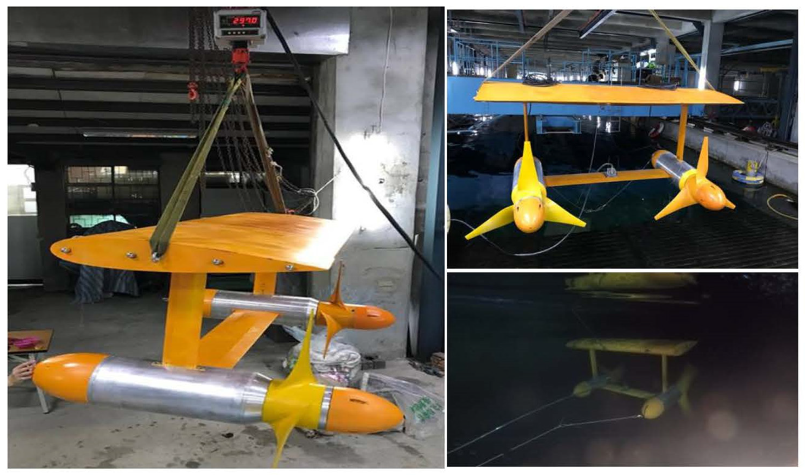
Figure 3.
Prototypes of NSYSU designed (a) floating nozzle-diffusor duct (NDD) power generation system (b) deployed successfully in the sea area near the Penghu cross-sea bridge in 2013.
Figure 3.
Prototypes of NSYSU designed (a) floating nozzle-diffusor duct (NDD) power generation system (b) deployed successfully in the sea area near the Penghu cross-sea bridge in 2013.
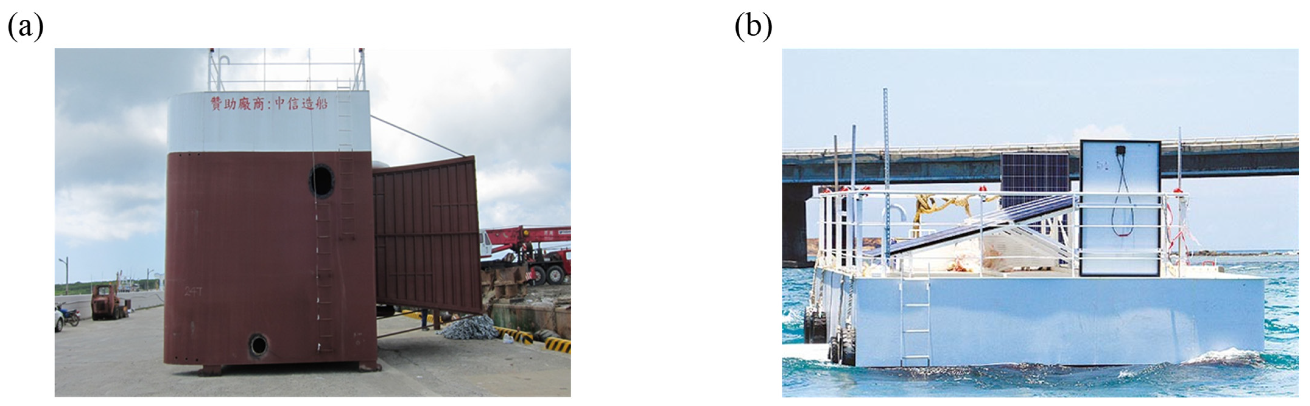
Figure 4.
(a) Three-dimensional diagram and (b) plan view of the duct used in the simulations.
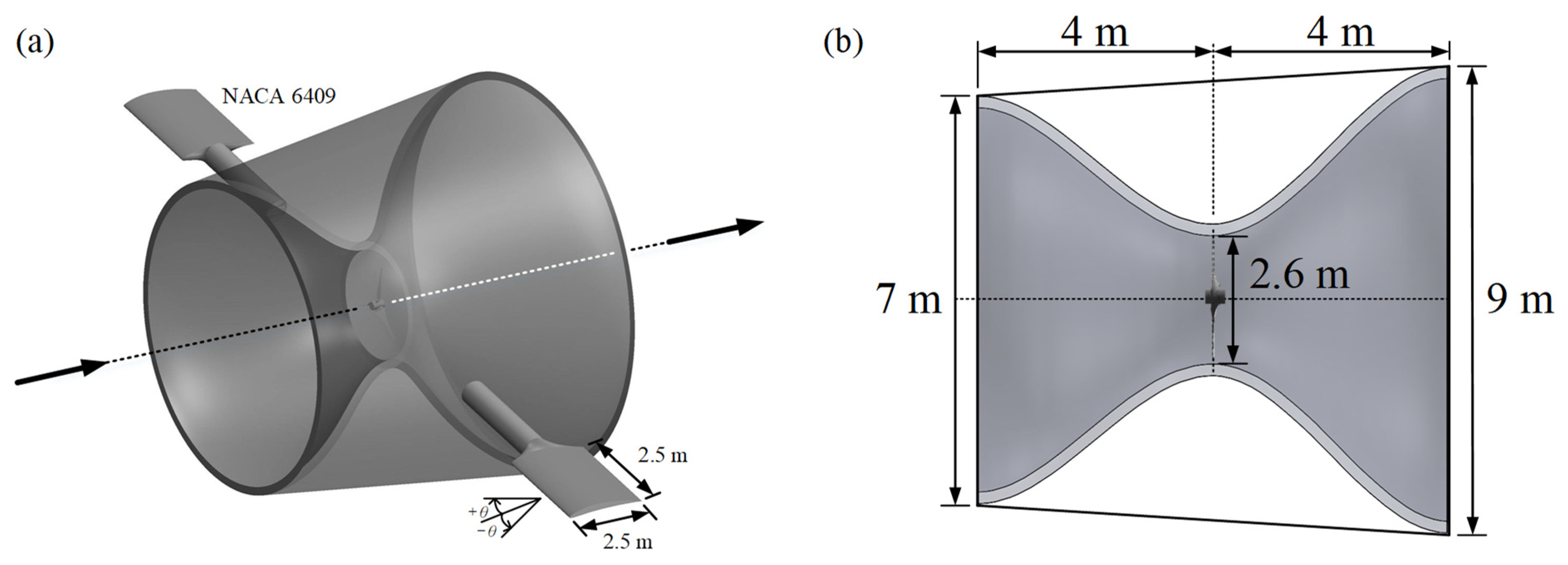
Figure 5.
Comparisons of simulated inline velocity of different domain lengths and mesh numbers: (a) upstream length (Lu), (b) downstream length (Ld), (c) side length (Ls), and (d) mesh size and growth rate. The computational domains for translational motions, D the nozzle inlet diameter.
Figure 5.
Comparisons of simulated inline velocity of different domain lengths and mesh numbers: (a) upstream length (Lu), (b) downstream length (Ld), (c) side length (Ls), and (d) mesh size and growth rate. The computational domains for translational motions, D the nozzle inlet diameter.
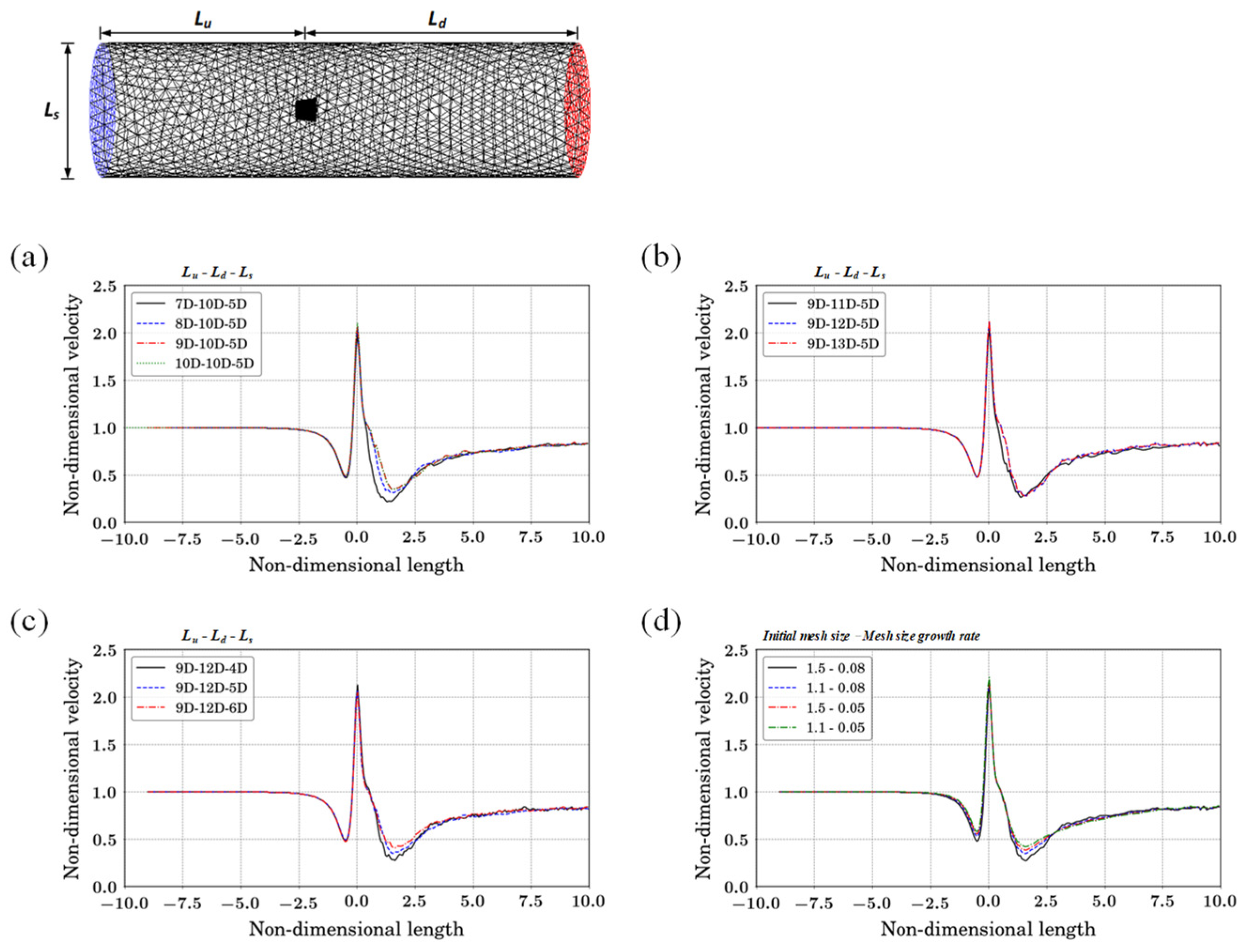
Figure 6.
Grid topology and finer mesh around the (a) duct and (b) turbine blades.

Figure 7.
The six degrees of freedom (6DoF) motions of an object.
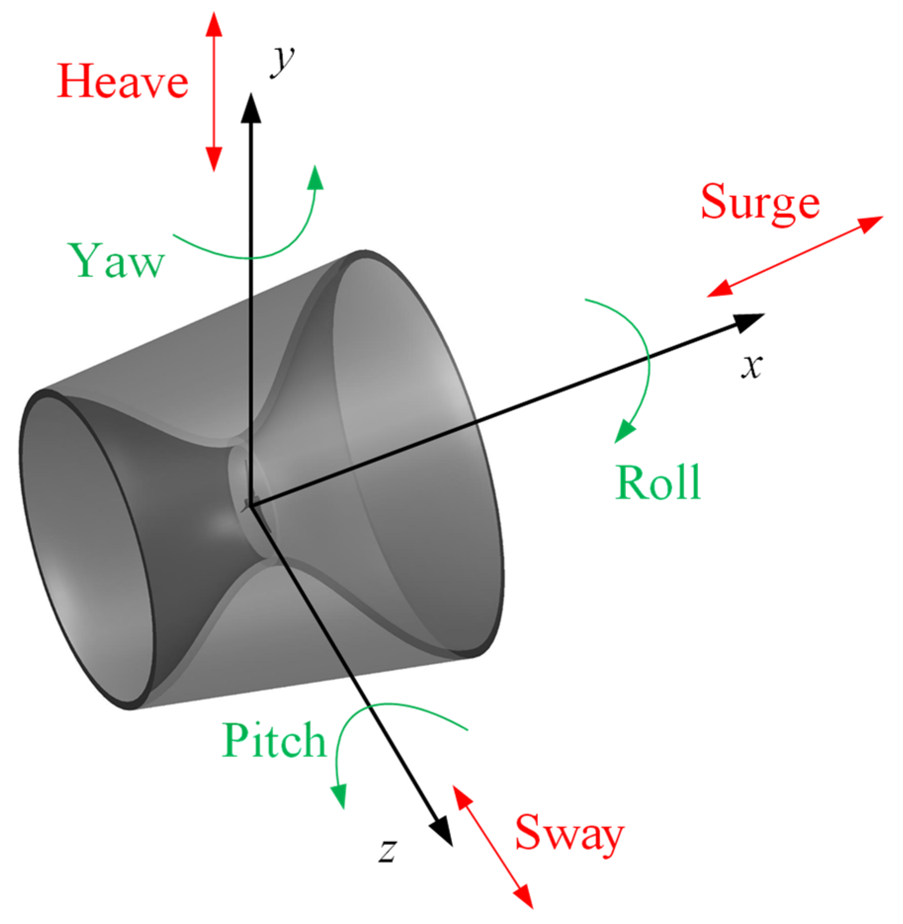
Figure 8.
The external force is received by the duct under the translational motion of six degrees of freedom (6DoF). (a) Surge; (b) Sway; (c) Heave. ○, simulation values; ―, Equation (10).
Figure 8.
The external force is received by the duct under the translational motion of six degrees of freedom (6DoF). (a) Surge; (b) Sway; (c) Heave. ○, simulation values; ―, Equation (10).
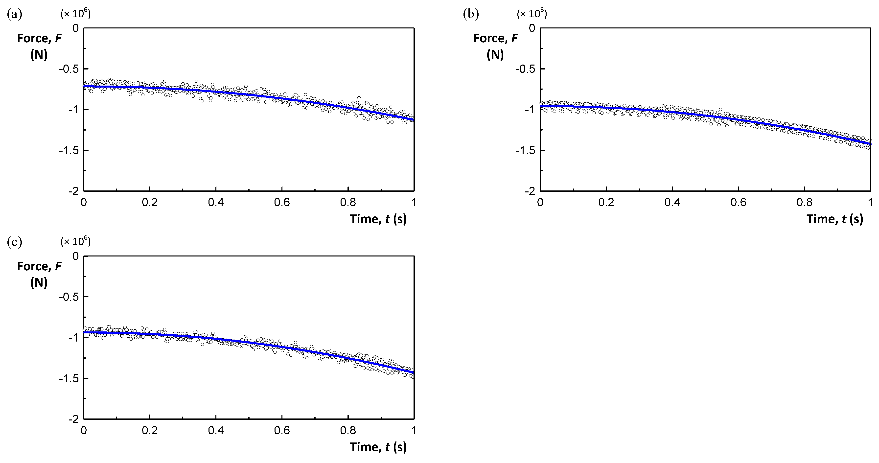
Figure 9.
External moment received by the duct under the rotational motion of six degrees of freedom (6DoF). (a) Roll; (b) Pitch; (c) Yaw. ○, simulation values; ―, Equation (13).
Figure 9.
External moment received by the duct under the rotational motion of six degrees of freedom (6DoF). (a) Roll; (b) Pitch; (c) Yaw. ○, simulation values; ―, Equation (13).
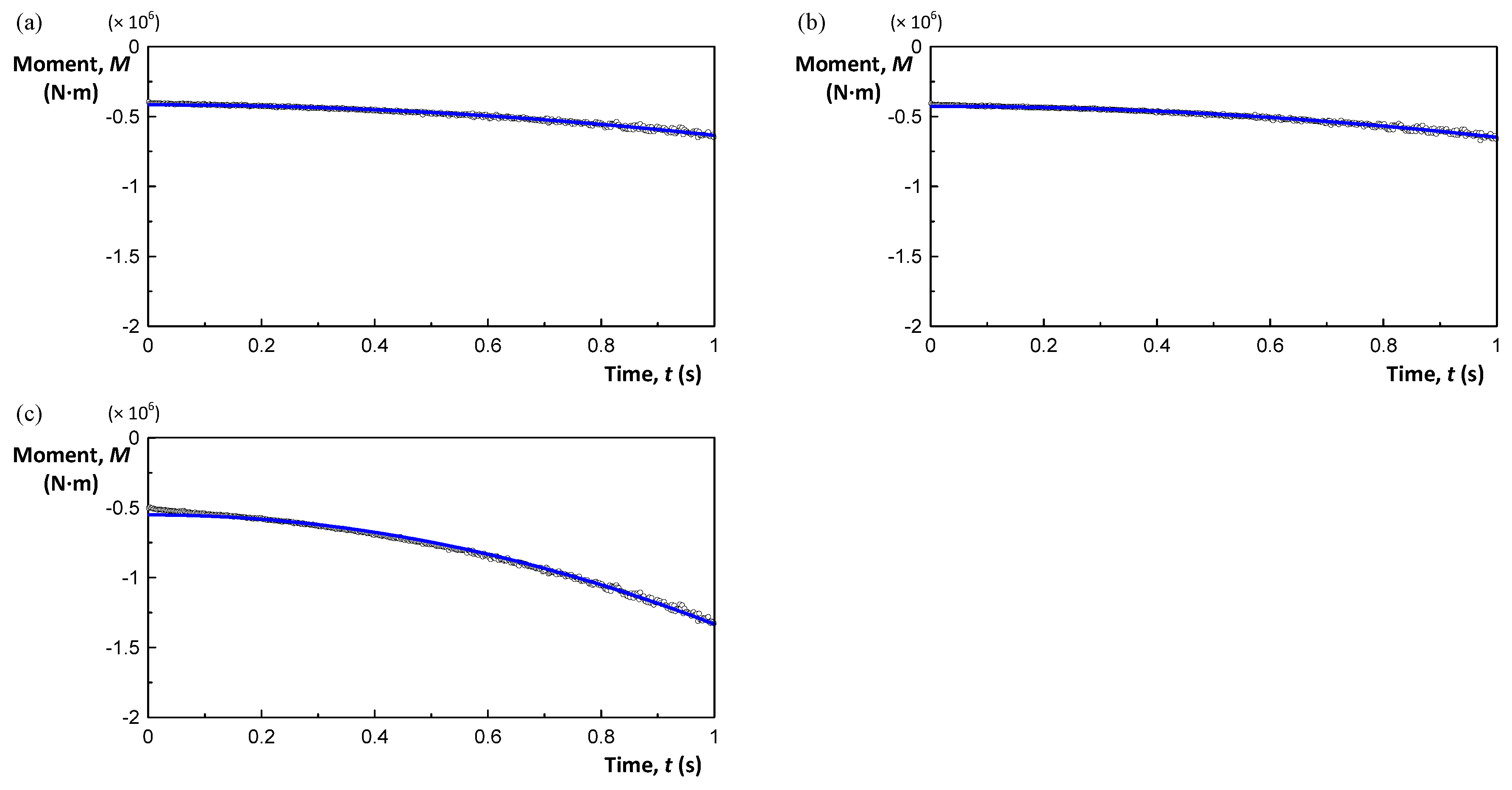
Figure 10.
Variation of the external force F(t) within the 1 s interval with different linear acceleration a.
Figure 10.
Variation of the external force F(t) within the 1 s interval with different linear acceleration a.
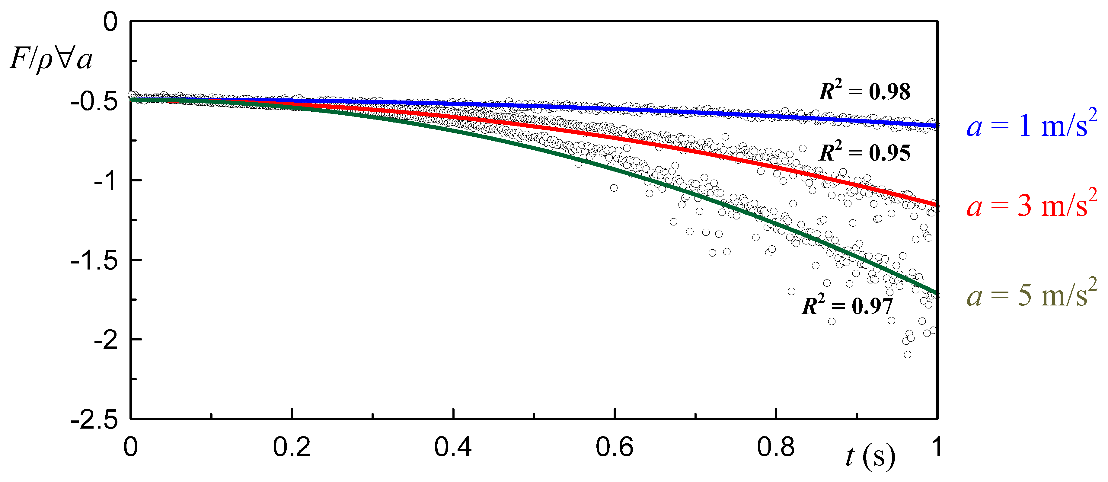
Figure 11.
Duct model in OrcaFlex.

Figure 12.
Illustration of single duct anchored on the seabed.
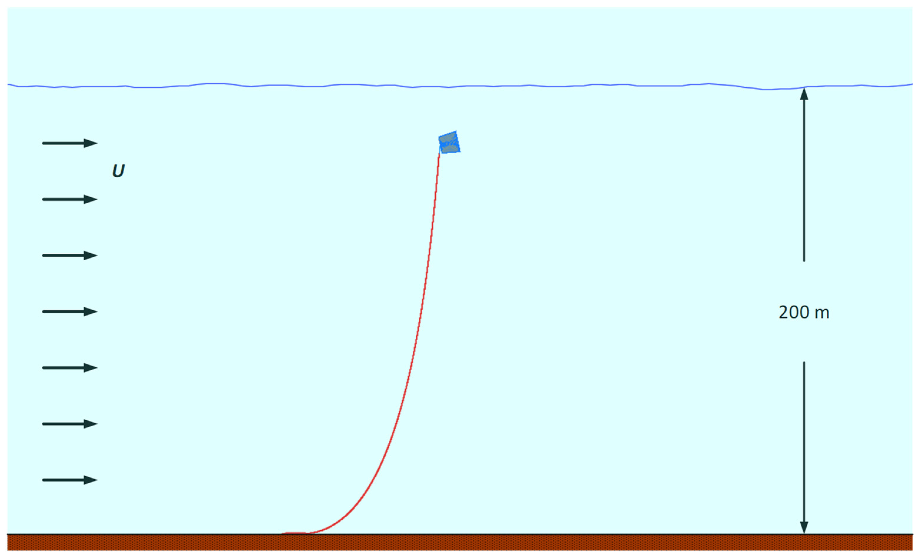
Figure 13.
(a) CB position on the local coordinate system of the duct model; (b) force balance and the corresponding position of CG.
Figure 13.
(a) CB position on the local coordinate system of the duct model; (b) force balance and the corresponding position of CG.
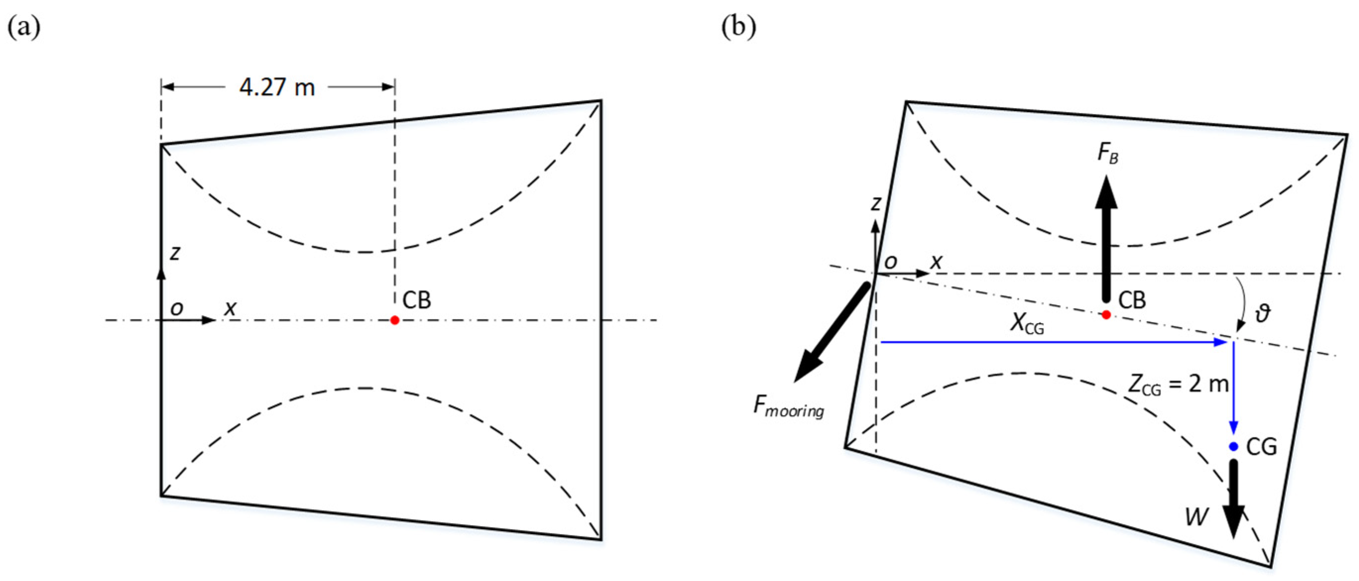
Figure 14.
Variation of the pitch angle θ according to different values of XCG for each duct weight. (a) 90%; (b) 87.5%; (c) 85%; (d) 82.5% of the duct buoyancy.
Figure 14.
Variation of the pitch angle θ according to different values of XCG for each duct weight. (a) 90%; (b) 87.5%; (c) 85%; (d) 82.5% of the duct buoyancy.
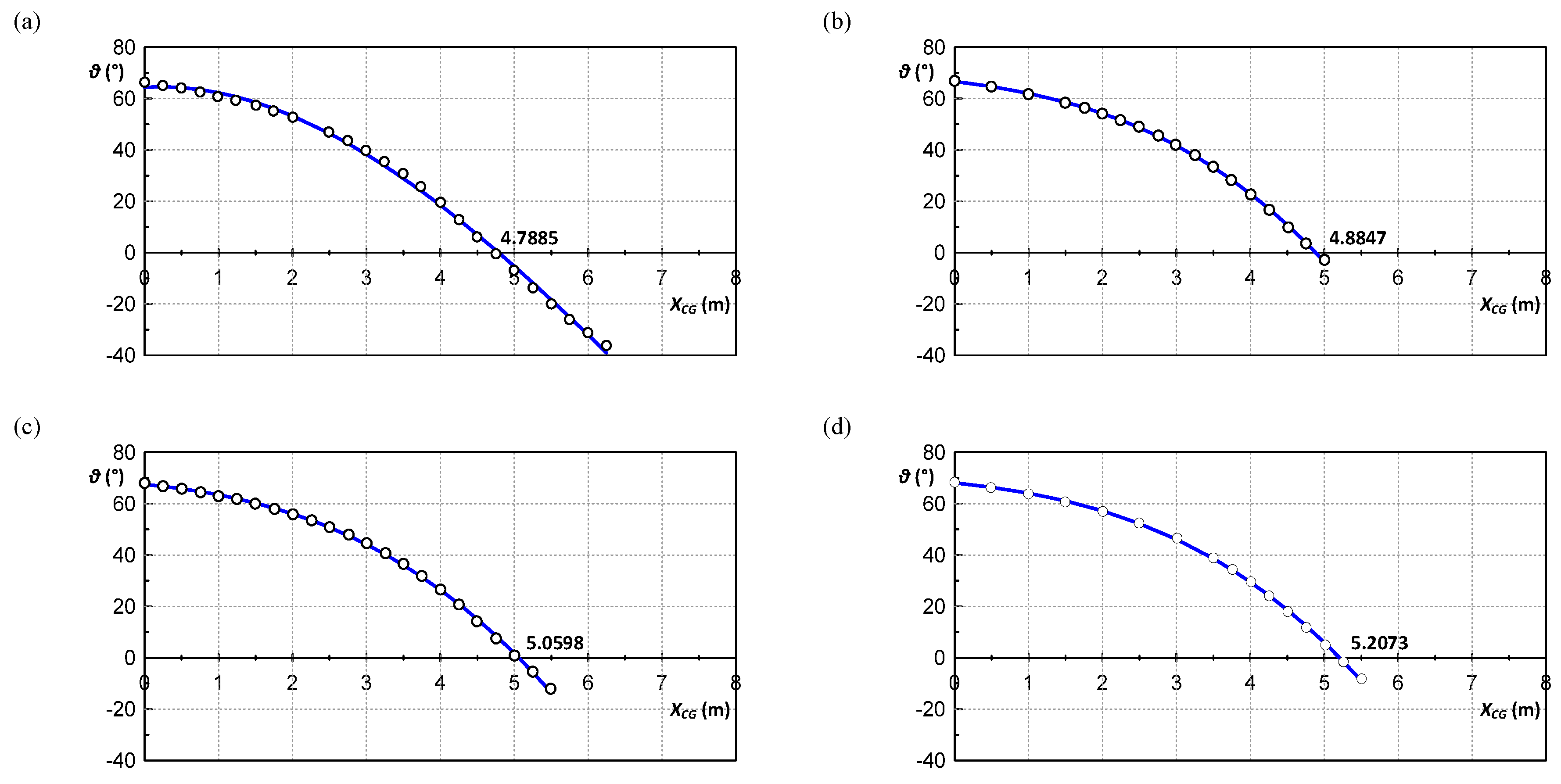
Figure 15.
(a) Experimental result for the neutral position of the duct by different attack angle of the wings [16]; (b) submerged depth with different design weight of the duct.
Figure 15.
(a) Experimental result for the neutral position of the duct by different attack angle of the wings [16]; (b) submerged depth with different design weight of the duct.
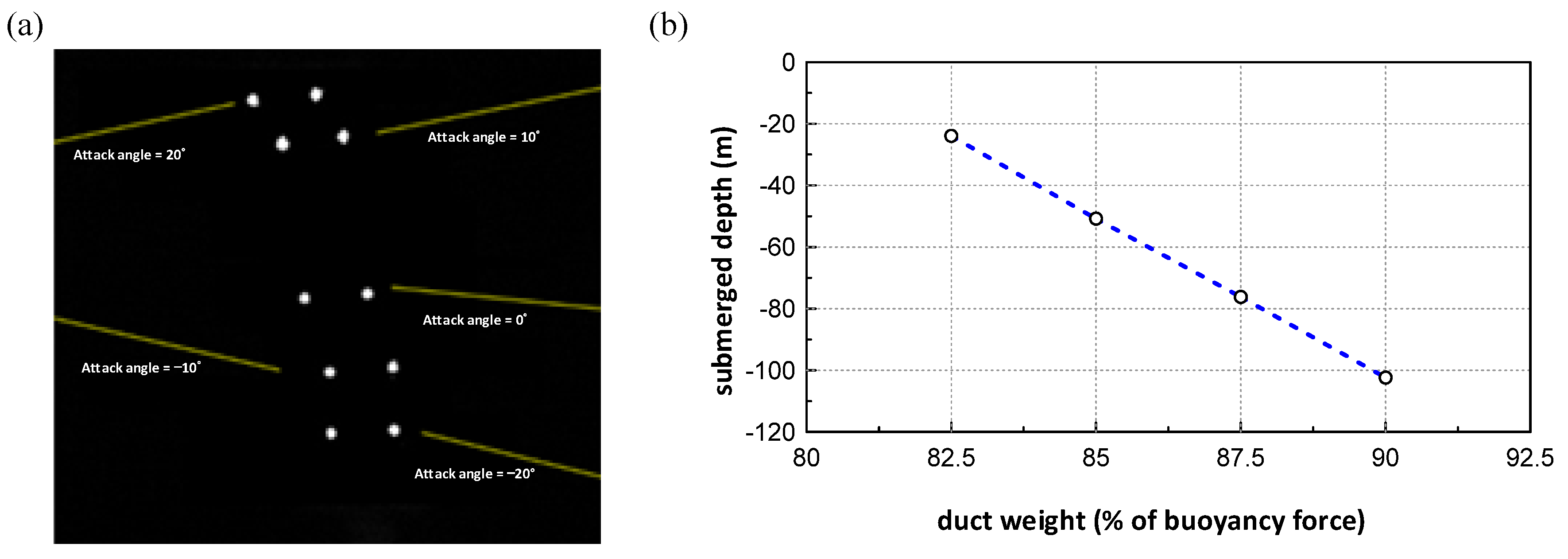
Figure 16.
Waveform of JONSWAP spectrum under normal wave condition.
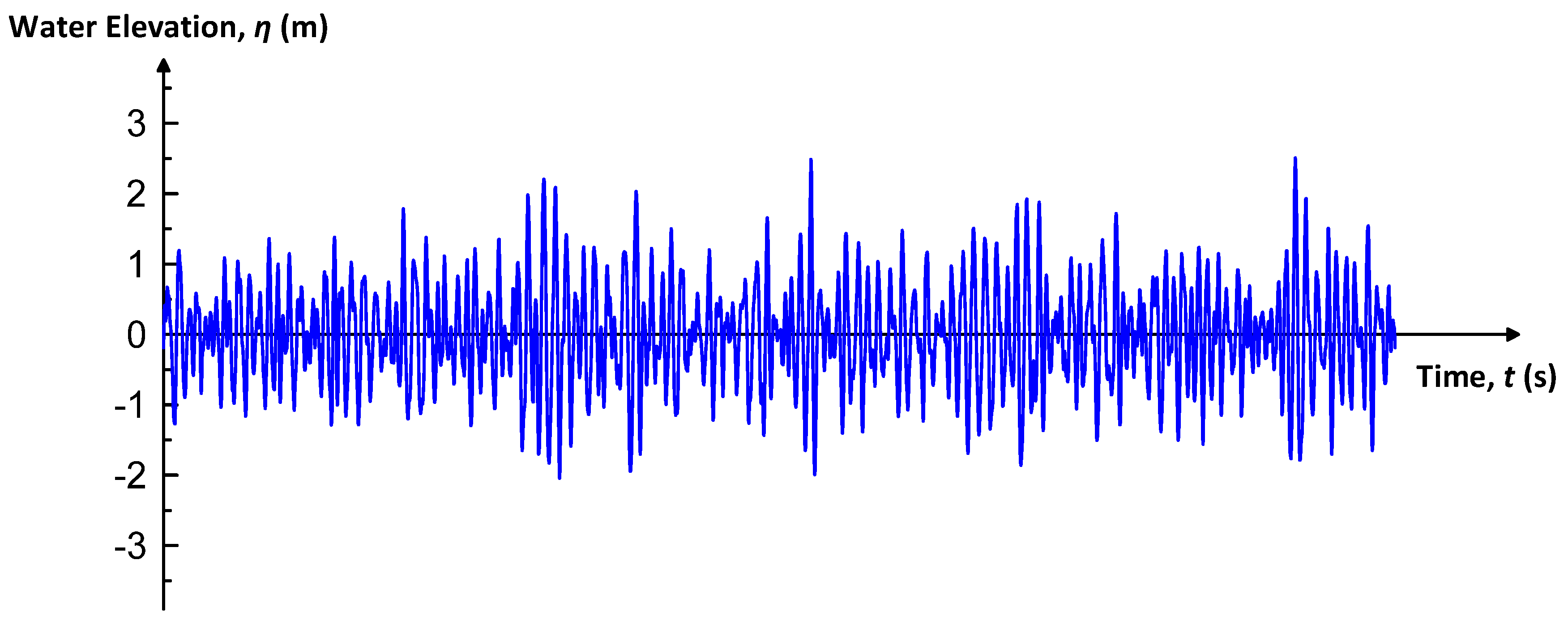
Figure 17.
Translational responses against different approaching wave directions under normal wave conditions. (a) Surge; (b) Sway; (c) Heave.
Figure 17.
Translational responses against different approaching wave directions under normal wave conditions. (a) Surge; (b) Sway; (c) Heave.
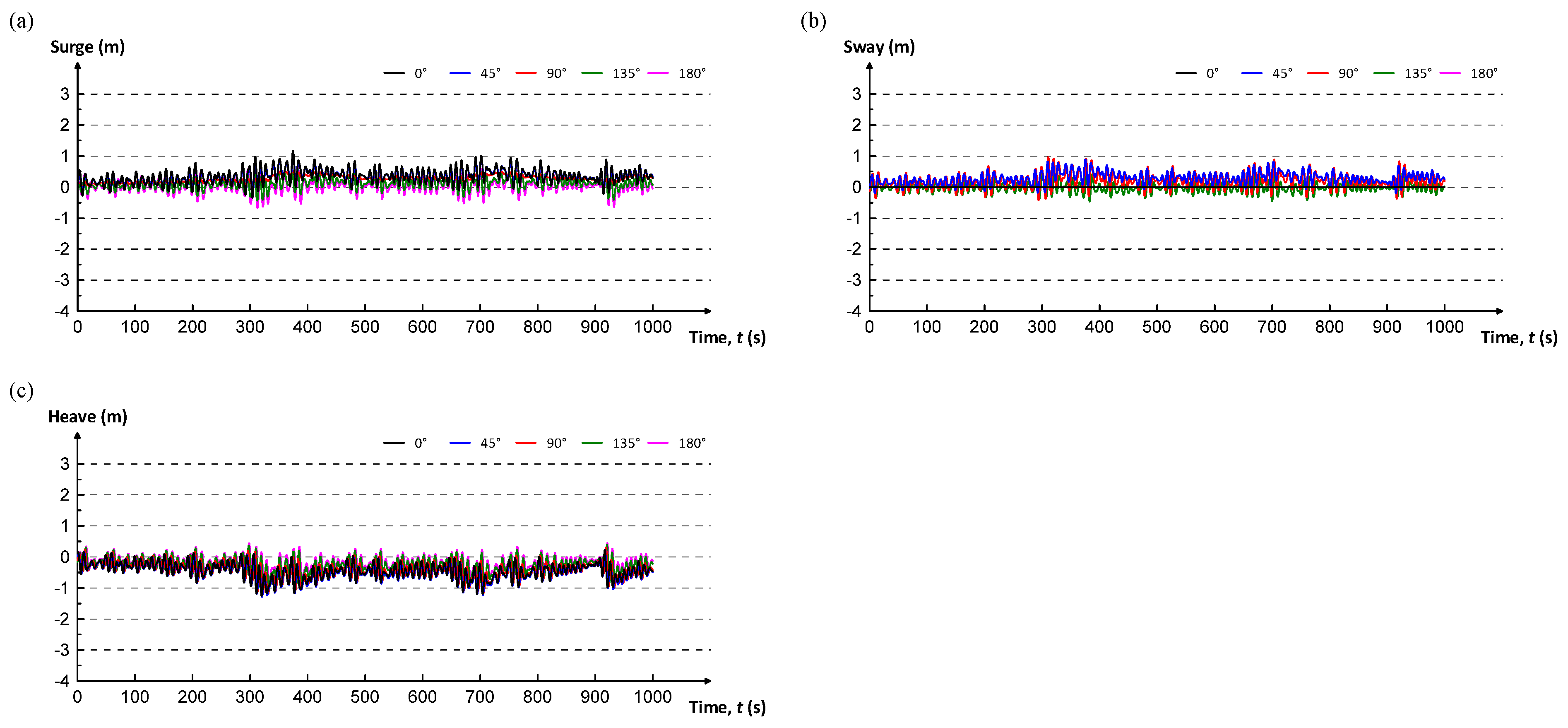
Figure 18.
Rotational responses against different approaching wave directions under normal wave conditions. (a) Roll; (b) Pitch; (c) Yaw.
Figure 18.
Rotational responses against different approaching wave directions under normal wave conditions. (a) Roll; (b) Pitch; (c) Yaw.
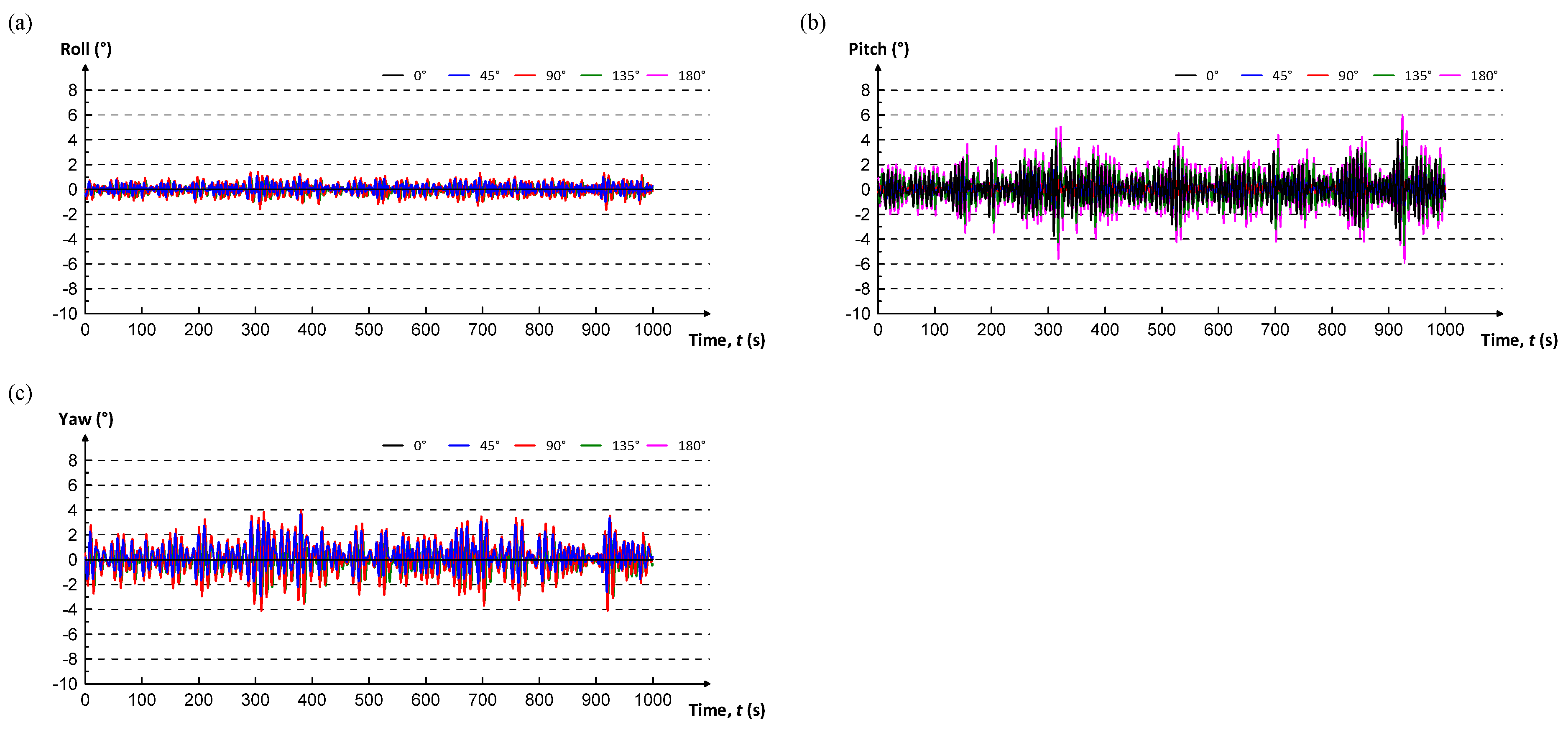
Figure 19.
Historical typhoon tracks around Taiwan from 1897–2017.
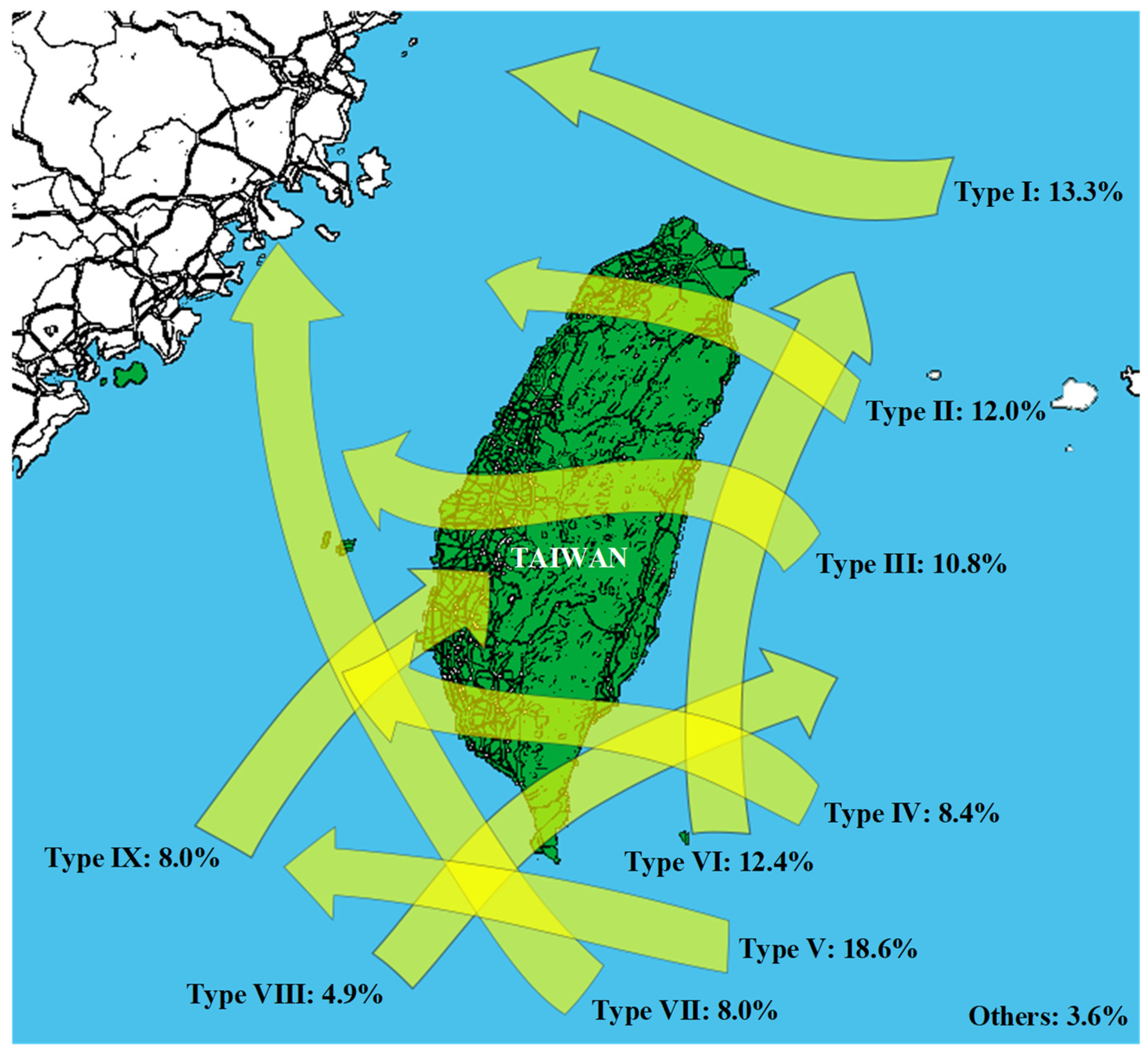
Figure 20.
Waveform of JONSWAP spectrum under storm wave condition.
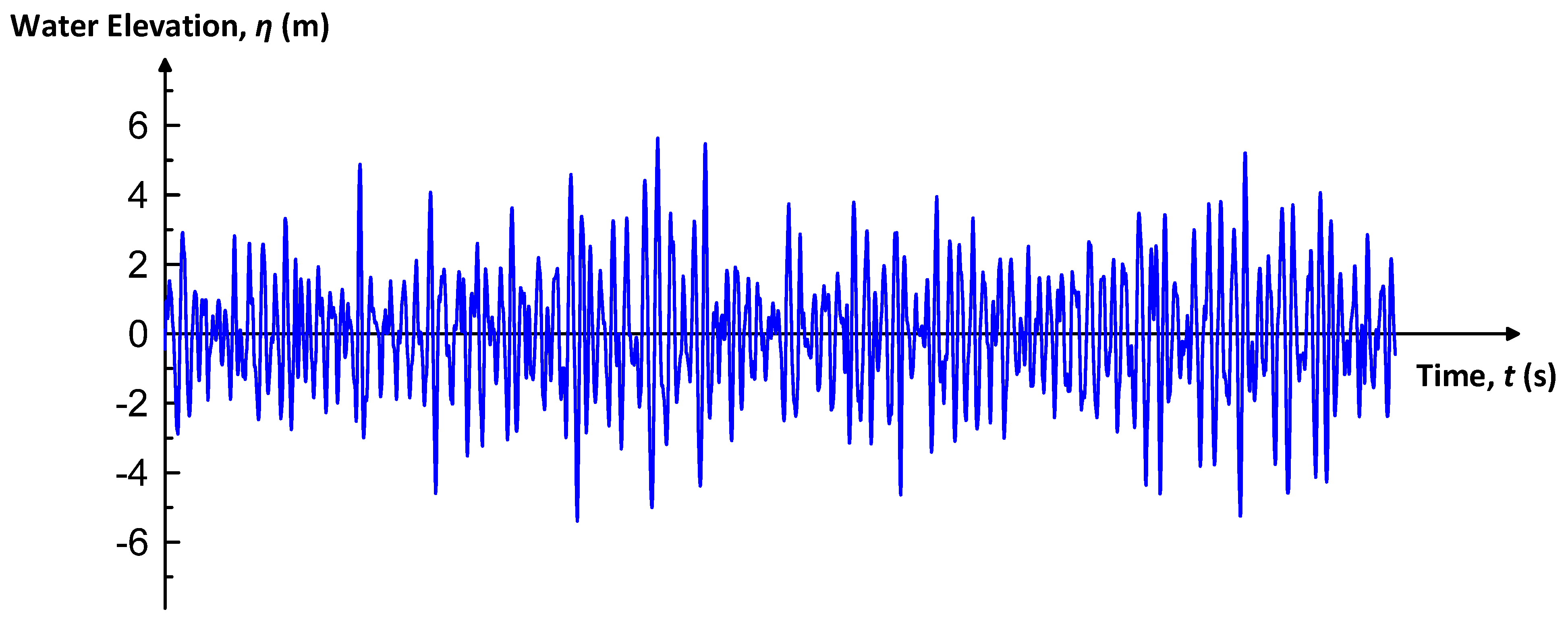
Figure 21.
Translational responses against different approaching wave directions under storm wave conditions. (a) Surge; (b) Sway; (c) Heave. Duct is 25 m below sea surface.
Figure 21.
Translational responses against different approaching wave directions under storm wave conditions. (a) Surge; (b) Sway; (c) Heave. Duct is 25 m below sea surface.
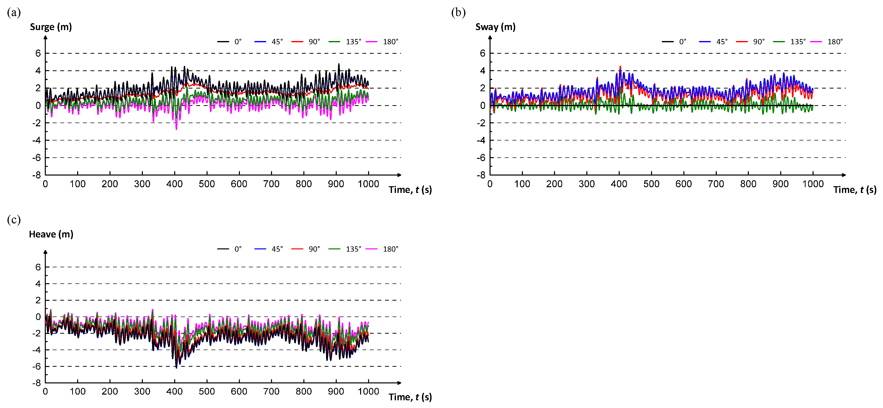
Figure 22.
Rotational responses against different approaching wave directions under storm wave conditions. (a) Roll; (b) Pitch; (c) Yaw. Duct is 25 m below sea surface.
Figure 22.
Rotational responses against different approaching wave directions under storm wave conditions. (a) Roll; (b) Pitch; (c) Yaw. Duct is 25 m below sea surface.

Figure 23.
Variation of yaw at different water depths against 90° storm waves.
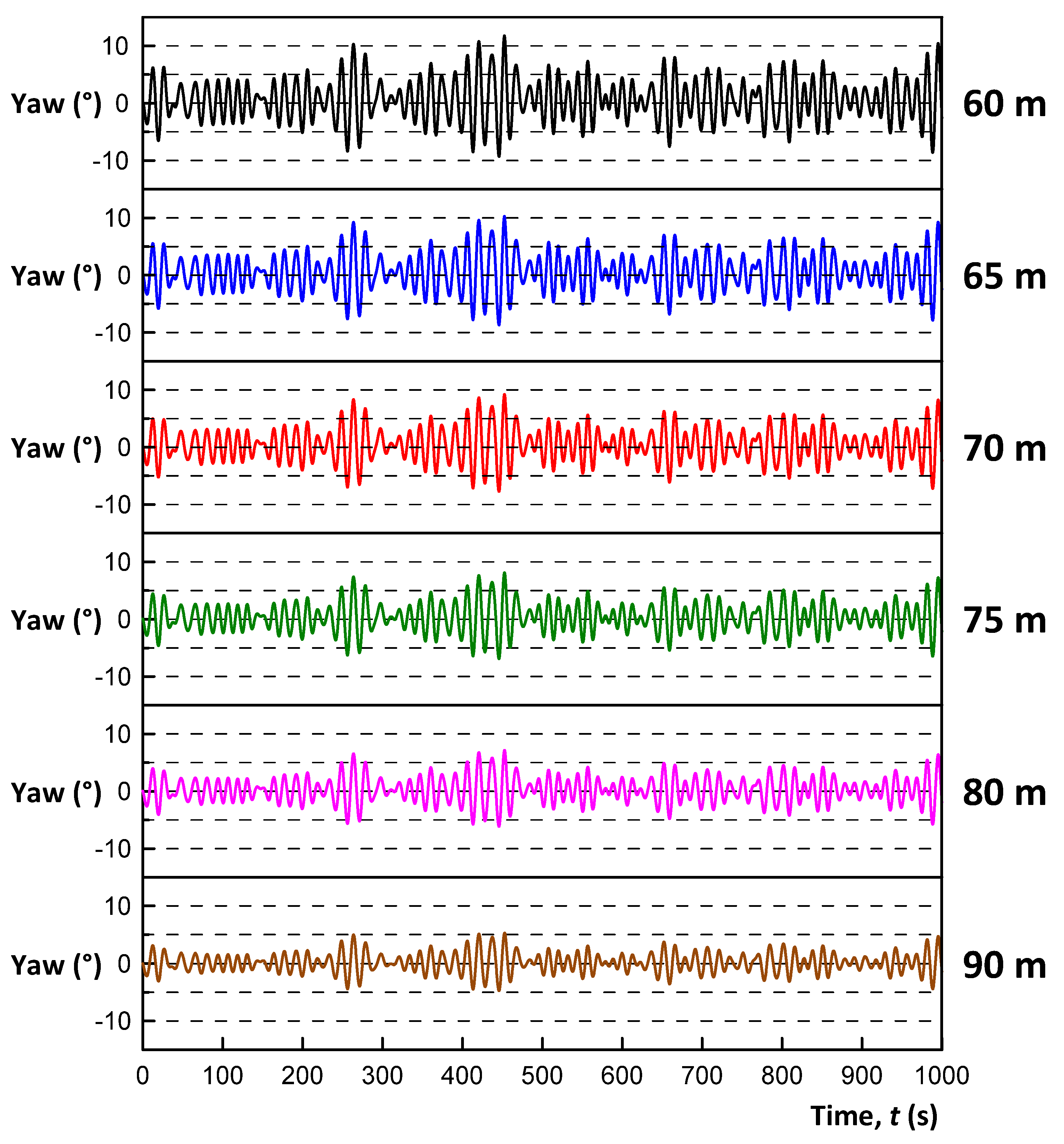
Figure 24.
The responses of duct in different dimensionless submerged depths.

Figure 25.
Optimized circular nozzle-diffuser duct designed by harmony search method.


Table 1.
Cd for the six degrees of freedom (6DoF).
| Surge | Sway | Heave | Pitch | Yaw | Roll | |
|---|---|---|---|---|---|---|
| Drag force (N) | 406,497 | 291,639 | 457,572 | |||
| Projected area (m2) | 67.28 | 67.20 | 78.96 | |||
| Drag moment (N-m) | 223,137 | 227,444 | 374,457 | |||
| Drag moment area (m5) | 2153 | 2572 | 7770 | |||
| Cd/Cdr | 1.31 | 0.94 | 1.26 | 5.06 | 4.31 | 2.35 |
Table 2.
Ca for the six degrees of freedom (6DoF).
| Added Mass (kg) | Added Moment of Inertia (kg·m2) | |||||
|---|---|---|---|---|---|---|
| Surge | Sway | Heave | Pitch | Yaw | Roll | |
| Value | 235,442 | 291,820 | 310,403 | 220,548 | 217,155 | 98,398 |
| Ca/Car | 0.69 | 0.86 | 0.91 | 0.65 | 0.64 | 0.29 |
Note: The mass of the displaced water is 339,305 kg.
Table 3.
Mooring line properties.
| Nominal diameter (m) | 0.133 |
| Diameter (m) | Outer = 0.24; Inner = 0 |
| Bending stiffness (kN·m2) | X = 0; Y = 0 |
| Axial stiffness (kN) | 1.52 × 10⁶ |
| Weight in air (kN/m) | 3.473 |
| Displacement (kN/m) | 0.455 |
| Weight in water (kN/m) | 3.018 |
| Diameter to weight ratio (m/kN) | 0.08 |
| Minimum breaking load (kN) | 15,984 |
| Poisson ratio | 0.5 |
| Drag coefficient (no axial drag) | 2.4 |
| Lift coefficient | 0 |
| Added mass coefficient (only axial direction) | 1 |
| Allowable tension (kN) | 15,984 |
Table 4.
JONSWAP parameters for normal and storm wave conditions around the Taitung area.
| γ | α | fp | |
|---|---|---|---|
| Normal wave condition | 1.59 | 0.0151 | 0.094 |
| Storm wave condition | 1.22 | 0.0047 | 0.105 |
Note: fp = spectrum peak frequency, γ and α are empirical parameters.
Publisher’s Note: MDPI stays neutral with regard to jurisdictional claims in published maps and institutional affiliations. |
© 2021 by the authors. Licensee MDPI, Basel, Switzerland. This article is an open access article distributed under the terms and conditions of the Creative Commons Attribution (CC BY) license (https://creativecommons.org/licenses/by/4.0/).
Share and Cite
MDPI and ACS Style
Yeh, P.-H.; Tsai, S.-Y.; Chen, W.-R.; Wu, S.-N.; Hsieh, M.-C.; Chen, B.-F. A Simple Nozzle-Diffuser Duct Used as a Kuroshio Energy Harvester. Processes 2021, 9, 1552. https://doi.org/10.3390/pr9091552
AMA Style
Yeh P-H, Tsai S-Y, Chen W-R, Wu S-N, Hsieh M-C, Chen B-F. A Simple Nozzle-Diffuser Duct Used as a Kuroshio Energy Harvester. Processes. 2021; 9(9):1552. https://doi.org/10.3390/pr9091552
Chicago/Turabian StyleYeh, Po-Hung, Shang-Yu Tsai, Wei-Ren Chen, Shing-Nan Wu, Meng-Chang Hsieh, and Bang-Fuh Chen. 2021. "A Simple Nozzle-Diffuser Duct Used as a Kuroshio Energy Harvester" Processes 9, no. 9: 1552. https://doi.org/10.3390/pr9091552
Note that from the first issue of 2016, this journal uses article numbers instead of page numbers. See further details here.