Regulation of Eukaryote Metabolism: An Abstract Model Explaining the Warburg/Crabtree Effect

Abstract

Adaptation of metabolism is a response of many eukaryotic cells to nutrient heterogeneity in the cell microenvironment. One of these adaptations is the shift from respiratory to fermentative metabolism, also called the Warburg/Crabtree effect. It is a response to a very high nutrient increase in the cell microenvironment, even in the presence of oxygen. Understanding whether this metabolic transition can result from basic regulation signals between components of the central carbon metabolism are the the core question of this work. We use an extension of the René Thomas modeling framework for representing the regulations between the main catabolic and anabolic pathways of eukaryotic cells, and formal methods for confronting models with known biological properties in different microenvironments. The formal model of the regulation of eukaryote metabolism defined and validated here reveals the conditions under which this metabolic phenotype switch occurs. It clearly proves that currently known regulating signals within the main components of central carbon metabolism can be sufficient to bring out the Warburg/Crabtree effect. Moreover, this model offers a general perspective of the regulation of the central carbon metabolism that can be used to study other biological questions.

1. Introduction

The status of the eukaryotic cell, such as quiescence and proliferation, highly depends on nutrient conditions in the microenvironment. In the presence of oxygen and scarcity of nutrients, a very efficient metabolism relying on the mitochondrial respiratory chain and the presence of electron acceptors (oxygen) can produce most of the chemical energy (ATP) out of sugar (glucose). In an abundance of nutrients, such efficient machinery is not necessary high, and ATP production turnover can be achieved by increasing the glycolysis rate, thanks to the increased glucose uptake rate, among others. A single enzyme in human cells (lactate dehydrogenase), can regenerate the redox cofactor ($NA{D}^{+}$) that is necessary for this inefficient but fast glycolytic process called fermentation [1].

For facultative fermentative cells, a metabolic shift occurs from an efficient (mitochondrial respiration) to an inefficient metabolism (fermentation) when passing from a poor to a rich milieu of glucose even in the presence of oxygen. This metabolic transition is known as the Warburg/Crabtree effect from the authors who first observed this glycolytic phenotype in tumors. This effect is also observed in microorganisms such as yeast (e.g., Saccharomyces Cerevisiae) and we are not distinguishing here the reversibility/irreversibility aspect of this metabolic shift which differentiates cancer cells from microorganisms.

A lot of studies have been devoted to the understanding of the Warburg/Crabtree effect from the molecular point of view [2,3,4,5]. These studies are all based on mathematical modeling using flux analyses, classical for metabolism. In these approaches, the metabolic switch is studied in terms of optimization functions tuned for different environments (hypoxia, glucose intake, etc.) without directly studying the regulatory mechanisms that control this switch. Such biochemical reaction models may hide the main regulations behind the indirect consequences of the chosen optimization functions. Here, we develop an original point of view as we seek to understand if the main regulations of the cell metabolism could be able to generate the Warburg/Crabtree effect. For this purpose, we make use of a regulation modeling formalism and, as the Warburg/Crabtree effect can be seen as an on/off mechanism, a priori non-quantitative, we adopt a discrete mathematical approach instead of continuous ones.

In this work, we ask whether the Warburg/Crabtree effect can be the result of systemic combinations of basic regulation signals of the main components of central carbon metabolism, or whether we need to evoke some specific and detailed molecular mechanism. Notice that we wrote “can be” instead of “is” in the previous sentence. Intrinsically a mathematical model never proves a biological phenotype, it only predicts possibly interesting cascades of effects (which can be experimentally refuted at any moment). More precisely, our mathematical model includes the main actors and their mutual regulations. According to our aim, we avoid modeling specific molecular mechanisms as such, to establish that the Warburg/Crabtree effect can be a consequence of only high-level regulations. Additionally, we only represent the main regulations that are common to a wide variety of eukaryote cell types, so that our result covers a rather wide scope. Obviously, as always in biology, there can be exceptions for some cell types.

To study the potential ability of the cell to perform fermentation in the presence of oxygen (with or without aerobic respiration), we focus on the regulation signals of the main catabolic and anabolic pathways of eukaryotic cells: glycolysis, fermentation, Krebs cycle, Oxidative Phosphorylation, lipidic and non-lipidic synthesis (e.g., pentose phosphate pathway) together with cofactors, and the most important nutrients. Our qualitative description of these components is accompanied by a precise description of regulation rules that govern or control the function of these components. We develop a qualitative coarse-grained model on purpose: only the main well-known metabolic pathways and cofactors are represented. Owing to this choice, the rules and parameters that govern the one-step direct influences of these components on each other are likely to be induced via classical or current biochemical literature. Nonetheless, more that 100 parameters were necessary, the identification of which took us several years of research, summarized here.

Once the model is set up using biological knowledge concerning the inter-component regulation signals (“local” knowledge), the systemic consequences of these local regulation rules, i.e., the emerging properties of the model (“global” cellular metabolic phenotypes) can be addressed rigorously. Even more, formal methods from computer science allows a fully computer-aided reasoning on emerging properties. Indeed, for more than one decade, these formal techniques have been developed to strongly assist modeling biological regulation networks [6,7]. They provide different automated procedures, both to prove the compatibility of the model with respect to biological observations (translated into a formal language), and to reveal underlying parameters.

We take benefit of the power of coupling, on the one hand, an extension of the R. Thomas’ modeling approach [8,9] with the additional expressiveness of multiplexes [10], and on the other hand, formal methods from computer science. This power is made effective through the associated platforms TotemBioNet [11,12] and DyMBioNet [13]. Here, this approach is used for the first time to design and formally validate a regulation model of the cell energetic metabolism, even if a precursory model has been introduced earlier in [14]. The classical regulation view of activation and inhibition signals can be interpreted here as “substrate producers” and “substrate consumers,” to abstract the underlying mass action rules that governs metabolic fluxes in term of regulations. Moreover, our model is designed to study the shift between the two metabolic regimes (respiration and fermentation), we focus less on the stationarity of these two regimes than on the global properties under different microenvironments (such as nutrient abundance or not).

All in all, the design of this model has been made possible for two reasons: a high level of description which allowed the determination of the majority of the parameter values from well-established biochemical knowledge, and a systematic use of formal methods to verify the cell phenotype specifications. The respiration/fermentation shift is involved in many cell behavior questions, so that our model of the central carbon metabolism constitutes a reusable reference model.

The basic concepts and proper methodology of discrete and formal modeling are reminded in Section 2. In this section, we quickly sketch out the theoretical background and corresponding methodology as well as tools for efficient algorithmic enumeration and verification. The basic concepts of metabolism regulation and Warburg/Crabtree effect are reminded in Section 3. Our abstract formal model of eukaryote metabolism regulation is presented in Section 4 where all variables and all regulations are characterized and formalized. Most of the parameter values is established in Section 5: Classical knowledge of biochemical aspects within the metabolic pathways are mostly sufficient to induce the parameter values. Section 6 describes the main cellular metabolic phenotypes in different environments (including the ones of the Warburg/Crabtree effect) and their translation into a formal language. Section 7 makes use of formal methods to extract the remaining parameters values to construct a model which is consistent with all phenotypes established in Section 6: It reveals all the parametrizations compatible with the Warburg/Crabtree properties, establishing consequently that the Warburg/Crabtree effect can be the result of the systemic combinations of basic regulation signals between the main components of central carbon metabolism. Lastly, Section 8 concludes.

2. Theoretical Background, Methods and Tools

A reader familiar with discrete modelling of regulation networks can skip this section. From the 1970s onwards, R. Thomas and co-workers developed a qualitative (discrete) method for abstracting biological regulation networks, which preserves compatibility with quantitative frameworks such as differential equations or stochastic approaches [8,9]. In particular, most of the complexity of dynamic system modeling resides in the entanglement of the feedback loops within the regulation graph. They are at the origin of the phenomena of homeostasis and multi-stationarity, and the Thomas’ method fully captures this complexity [15].

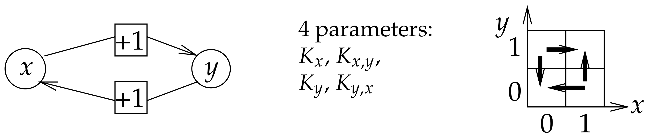
2.1. Interaction Graph

As for all regulation modeling frameworks, a model first relies on a directed interaction graph between variables that represent the main biochemical compounds and the main entities of the regulation network. Figure 1, Figure 2 and Figure 3 contain examples of such regulation graphs. The peculiarity of discrete modeling is that quantitative concentration levels, production speeds or levels of activity are abstracted into qualitative levels that are positive integers. This abstraction is based on well-chosen thresholds above which regulations take place: Thresholds are not chosen on a sort of “proportional” basis but according to the action they have on their different targets. If a variable x can possibly regulate n targets according to the regulation graph, then it keeps level 0 until its current activity (or concentration) level makes it able to regulate its first target, in which case it “jumps” to level 1. More generally, if the current activity level of x allows x to regulate m among its n targets, then its activity level is m by definition. Things are in fact a little bit more subtle because one can consider that several targets have the same threshold, in which case the maximal qualitative level of x will be strictly lower than n.

2.2. Dynamic Parameters

When modeling regulations, a major property is that the value toward which a variable tends, depends only on the inventory of the active regulations that it receives. This is encoded into the kinetic parameters. The action of a regulator of the variable can be qualified either active if it passes a given threshold, or inactive if it does not. Any potential resource can be active or inactive, thus this leads to a huge number of parameters because one needs to know the value toward which a variable tends for all possible combinations of its potential (active) resources: if a variable y has n predecessors $x_1$ to $x_n$ in the graph, then it has a priori $2^n$ possible combinations of its resources (all possible subsets $\omega$ of $\{x_1,\dots ,x_n\}$), thus $2^n$ parameters. We classically note $K_{\mathbf{y},\omega }$ the integer value toward which y tends, if we assume that its set of active resources is $\omega$ forever. In other words, $K_{\mathbf{y},\omega }$ is the number of targets regulated by y, after an infinite delay and if we assume that its set of active resources is $\omega$ forever.

Of course, “toward which” is crucial in the previous paragraph and $K_{\mathbf{y},\omega }$ denotes what is usually called a local behavior. In the global behavior, during the necessary delay for y to move toward $K_{\mathbf{y},\omega }$, the set of resources $\omega$ has changed, so that before reaching $K_{\mathbf{y},\omega }$, the level of y is attracted toward a new $K_{\mathbf{y},{\omega }^{\prime }}$ which has no reason to be in the same direction than $K_{\mathbf{y},\omega }$. This succession of different attraction values finally build the global behavior of the mathematical model. The precise mathematical definitions of the global behavior can be found in [6,8] for example.

2.3. Formal Validation

Our goal is to build and validate as much as possible a mathematical model that mimics a real complex system. One consequently must distinguish local behavior (inferred about the fate of a chemical species if all others are “frozen”) and global behavior (the systemic evolution of some species, such as homeostasis or multistationary). Of course, local and global behaviors are not independent of each other in the existing real model, simply because the local behaviors entail the global one as emerging properties. Nevertheless, the point here is to formalize as suitably as possible the real system into a mathematical model and the validation step consists of verifying whether the global behavior of the mathematical model, which results entirely from the locally encoded local rules (via parameter values), reflects the intended global behavior of the real system. If not, it would mean that either the local behaviors or the global behavior have been erroneously formalized. The goal of the validation step is precisely to verify this consistency.

Here, information about the local behavior is encoded in terms of parameter values, which can be evaluated through reasoning on the basis of general biochemical knowledge, and information about the global behavior is represented in a validation matrix in which each formula expresses the temporal global behavior a variable must exhibit in a given environmental context. These two kinds of information (that will be summarized later on in

Table 1. Kinetic parameter values from Section 5.2. Only 7 parameter values remain free: $K_{\mathit{ATP},\mathbf{LBP}\mathbf{PHOX}}$, $K_{\mathit{ATP},\mathbf{GLYC}\mathbf{1}\mathbf{LBP}}$, $K_{\mathit{ATP},\mathbf{GLYC}\mathbf{1}\mathbf{GLYC}\mathbf{2}\mathbf{LBP}}$, $K_{\mathit{ATP},\mathbf{GLYC}\mathbf{1}\mathbf{LBP}\mathbf{PHOX}}$, $K_{\mathit{ATP},\mathbf{GLYC}\mathbf{1}\mathbf{GLYC}\mathbf{2}\mathbf{LBP}\mathbf{PHOX}}$, $K_{\mathit{NADH},\mathbf{FERM}\mathbf{GLYC}\mathbf{PHOX}}$ and $K_{\mathit{NADH},\mathbf{FERM}\mathbf{GLYC}\mathbf{KREBS}}$.

# Parameters for ATP	# Parameters for O2	# Parameters for NADH
$K_{\mathit{ATP}}=0$	$K_{\mathit{O}\mathit{2}}=0$	$K_{\mathit{NADH}}=0$
$K_{\mathit{ATP},\mathbf{LBP}}=0$	$K_{\mathit{O}\mathit{2},\mathbf{PHOX}}=0$	$K_{\mathit{NADH},\mathbf{FERM}}=0$
$K_{\mathit{ATP},\mathbf{nLBP}}=0$	$K_{\mathit{O}\mathit{2},\mathbf{exO}\mathbf{2}}=1$	$K_{\mathit{NADH},\mathbf{PHOX}}=0$
$K_{\mathit{ATP},\mathbf{LBP}\mathbf{nLBP}}=0$	$K_{\mathit{O}\mathit{2},\mathbf{exO}\mathbf{2}\mathbf{PHOX}}=1$	$K_{\mathit{NADH},\mathbf{AAS}}=0$
$K_{\mathit{ATP},\mathbf{PHOX}}=1$		$K_{\mathit{NADH},\mathbf{FERM}\mathbf{PHOX}}=0$
$K_{\mathit{ATP},\mathbf{nLBP}\mathbf{PHOX}}=1$	# Parameters for GLYC	$K_{\mathit{NADH},\mathbf{FERM}\mathbf{AAS}}=0$
$K_{\mathit{ATP},\mathbf{LBP}\mathbf{nLBP}\mathbf{PHOX}}=2$	$K_{\mathit{GLYC}}=0$	$K_{\mathit{NADH},\mathbf{AAS}\mathbf{PHOX}}=0$
$K_{\mathit{ATP},\mathbf{GLYC}\mathbf{1}}=0$	$K_{\mathit{GLYC},\mathbf{GR}}=0$	$K_{\mathit{NADH},\mathbf{FERM}\mathbf{AAS}\mathbf{PHOX}}=0$
$K_{\mathit{ATP},\mathbf{GLYC}\mathbf{1}\mathbf{nLBP}}=0$	$K_{\mathit{GLYC},\mathbf{GLC}\mathbf{1}}=0$	$K_{\mathit{NADH},\mathbf{FERM}\mathbf{KREBS}\mathbf{AAS}}=0$
$K_{\mathit{ATP},\mathbf{GLYC}\mathbf{1}\mathbf{LBP}\mathbf{nLBP}}=2$	$K_{\mathit{GLYC},\mathbf{GLC}\mathbf{1}\mathbf{GR}}=0$	$K_{\mathit{NADH},\mathbf{GLYC}\mathbf{AAS}\mathbf{PHOX}}=0$
$K_{\mathit{ATP},\mathbf{GLYC}\mathbf{1}\mathbf{GLYC}\mathbf{2}}=1$	$K_{\mathit{GLYC},\mathbf{GLC}\mathbf{1}\mathbf{GLC}\mathbf{2}}=0$	$K_{\mathit{NADH},\mathbf{GLYC}\mathbf{FERM}\mathbf{AAS}\mathbf{PHOX}}=1$
$K_{\mathit{ATP},\mathbf{GLYC}\mathbf{1}\mathbf{GLYC}\mathbf{2}\mathbf{nLBP}}=1$	$K_{\mathit{GLYC},\mathbf{GLC}\mathbf{1}\mathbf{GLC}\mathbf{2}\mathbf{GR}}=0$	$K_{\mathit{NADH},\mathbf{KREBS}\mathbf{FERM}\mathbf{AAS}\mathbf{PHOX}}=1$
$K_{\mathit{ATP},\mathbf{GLYC}\mathbf{1}\mathbf{GLYC}\mathbf{2}\mathbf{LBP}\mathbf{nLBP}}=2$	$K_{\mathit{GLYC},\mathbf{COF}}=0$	$K_{\mathit{NADH},\mathbf{GLYC}\mathbf{KREBS}\mathbf{FERM}\mathbf{AAS}\mathbf{PHOX}}=1$
$K_{\mathit{ATP},\mathbf{GLYC}\mathbf{1}\mathbf{PHOX}}=1$	$K_{\mathit{GLYC},\mathbf{COF}\mathbf{GR}}=0$	$K_{\mathit{NADH},\mathbf{GLYC}\mathbf{KREBS}\mathbf{AAS}}=0$
$K_{\mathit{ATP},\mathbf{GLYC}\mathbf{1}\mathbf{nLBP}\mathbf{PHOX}}=1$	$K_{\mathit{GLYC},\mathbf{COF}\mathbf{GLC}\mathbf{1}}=0$	$K_{\mathit{NADH},\mathbf{FERM}\mathbf{GLYC}\mathbf{AAS}}=0$
$K_{\mathit{ATP},\mathbf{GLYC}\mathbf{1}\mathbf{LBP}\mathbf{nLBP}\mathbf{PHOX}}=2$	$K_{\mathit{GLYC},\mathbf{COF}\mathbf{GLC}\mathbf{1}\mathbf{GR}}=1$	$K_{\mathit{NADH},\mathbf{GLYC}\mathbf{KREBS}}=0$
$K_{\mathit{ATP},\mathbf{GLYC}\mathbf{1}\mathbf{GLYC}\mathbf{2}\mathbf{PHOX}}=1$	$K_{\mathit{GLYC},\mathbf{COF}\mathbf{GLC}\mathbf{1}\mathbf{GLC}\mathbf{2}}=1$	$K_{\mathit{NADH},\mathbf{FERM}\mathbf{KREBS}}=0$
$K_{\mathit{ATP},\mathbf{GLYC}\mathbf{1}\mathbf{GLYC}\mathbf{2}\mathbf{nLBP}\mathbf{PHOX}}=1$	$K_{\mathit{GLYC},\mathbf{COF}\mathbf{GLC}\mathbf{1}\mathbf{GLC}\mathbf{2}\mathbf{GR}}=2$	$K_{\mathit{NADH},\mathbf{KREBS}\mathbf{AAS}}=0$
$K_{\mathit{ATP},\mathbf{GLYC}\mathbf{1}\mathbf{GLYC}\mathbf{2}\mathbf{LBP}\mathbf{nLBP}\mathbf{PHOX}}=2$		$K_{\mathit{NADH},\mathbf{GLYC}\mathbf{AAS}}=0$
	# Parameters for nLBP	$K_{\mathit{NADH},\mathbf{GLYC}\mathbf{PHOX}}=0$
# Parameters for LBP	$K_{\mathit{nLBP}}=0$	$K_{\mathit{NADH},\mathbf{FERM}\mathbf{GLYC}}=0$
$K_{\mathit{LBP}}=0$	$K_{\mathit{nLBP},\mathbf{PPP}}=1$	$K_{\mathit{NADH},\mathbf{KREBS}}=0$
$K_{\mathit{LBP},\mathbf{LS}}=1$	$K_{\mathit{nLBP},\mathbf{AAS}}=1$	$K_{\mathit{NADH},\mathbf{GLYC}}=0$
$K_{\mathit{LBP},\mathbf{BOX}}=0$	$K_{\mathit{nLBP},\mathbf{AAS}\mathbf{PPP}}=1$	$K_{\mathit{NADH},\mathbf{FERM}\mathbf{GLYC}\mathbf{KREBS}\mathbf{AAS}}=1$
$K_{\mathit{LBP},\mathbf{LS}\mathbf{BOX}}=1$		$K_{\mathit{NADH},\mathbf{KREBS}\mathbf{PHOX}}=1$
	# Parameters for KREBS	$K_{\mathit{NADH},\mathbf{KREBS}\mathbf{FERM}\mathbf{PHOX}}=1$
# Parameters for NCD	$K_{\mathit{KREBS}}=0$	$K_{\mathit{NADH},\mathbf{KREBS}\mathbf{AAS}\mathbf{PHOX}}=1$
$K_{\mathit{NCD}}=0$	$K_{\mathit{KREBS},\mathbf{AnO}}=1$	$K_{\mathit{NADH},\mathbf{GLYC}\mathbf{KREBS}\mathbf{PHOX}}=1$
$K_{\mathit{NCD},\mathbf{KREBS}}=0$	$K_{\mathit{KREBS},\mathbf{AnO}\alpha -\mathbf{KG}}=2$	$K_{\mathit{NADH},\mathbf{FERM}\mathbf{GLYC}\mathbf{KREBS}\mathbf{PHOX}}=1$
$K_{\mathit{NCD},\mathbf{AA}\mathbf{1}}=1$	$K_{\mathit{KREBS},\mathbf{BOX}}=1$	$K_{\mathit{NADH},\mathbf{GLYC}\mathbf{KREBS}\mathbf{AAS}\mathbf{PHOX}}=1$
$K_{\mathit{NCD},\mathbf{AA}\mathbf{1}\mathbf{KREBS}}=1$
$K_{\mathit{NCD},\mathbf{AA}\mathbf{1}\mathbf{AA}\mathbf{2}}=2$	# Parameters for PHOX	# Parameters for FERM
$K_{\mathit{NCD},\mathbf{AA}\mathbf{1}\mathbf{AA}\mathbf{2}\mathbf{KREBS}}=2$	$K_{\mathit{PHOX}}=0$	$K_{\mathit{FERM}}=0$
	$K_{\mathit{PHOX},\mathbf{PC}}=1$	$K_{\mathit{FERM},\mathbf{EP}}=1$

and 

Table 2. Validation matrix for the cell metabolism regulation model. Each row (resp. column) represents an experimental condition (resp. an observable systemic variable). Thus, each box of the table formalizes the known behavior of that observable variable in that experimental condition. Grey boxes refer to missing knowledge depending on the cell type or more generally knowledge which we do not consider as consensus. Lines 16, 17, 18, 34, 35 and 36 formalize the Warburg/Crabtree effect.

Biological Context	FA	exO2	GLC	AA	ATP (0–2)	O2 (0–1)	GLYC (0–2)	nLBP (0–1)	LBP (0–1)	FERM (0–1)	KREBS (0–2)	PHOX (0–1)	NADH (0–1)
					Neither lipids nor oxygen supply
1	0	0	0	0	td(0)	td(0)	td(0)	td(0)	td(0)	td(0)	td(0)	td(0)	td(0)
2 & 3	0	0	0	1 & 2		td(0)
4	0	0	1	0	!td(0)	td(0)	osc(0-1)			!td(0)		td(0)	osc
5	0	0	1	1	osc	td(0)	osc(0-1)	!td(0)		!td(0)		td(0)	osc
6	0	0	1	2	osc	td(0)	osc	!td(0)	!td(0)	!td(0)		td(0)	osc
7	0	0	2	0	!td(0)	td(0)	osc			!td(0)		td(0)	osc
8	0	0	2	1	osc	td(0)	osc	!td(0)		!td(0)		td(0)	osc
9	0	0	2	2	osc	td(0)	osc	!td(0)	!td(0)	!td(0)		td(0)	osc
					No lipids but oxygen supply
10	0	1	0	0	td(0)	!td(0)	td(0)	td(0)	td(0)	td(0)	td(0)	td(0)	td(0)
11 & 12	0	1	0	1 & 2		!td(0)
13	0	1	1	0	!td(0)	osc	osc			td(0)	osc	osc	osc
14	0	1	1	1	osc	osc	osc	!td(0)		td(0)	osc	osc	osc
15	0	1	1	2	osc	osc	osc	!td(0)	!td(0)	td(0)	osc	osc	osc
16	0	1	2	0	!td(0)	!td(0)	osc			!td(0)		!td(1)	osc
17 & 18	0	1	2	1&2	osc	!td(0)	osc	!td(0)	!td(0)	!td(0)		!td(1)	osc
					Lipids but no oxygen supply
19	1	0	0	0	td(0)	td(0)	td(0)	td(0)	td(0)	td(0)	td(0)	td(0)	td(0)
20 & 21	1	0	0	1 & 2		td(0)
22	1	0	1	0	osc	td(0)	osc(0-1)		!td(0)	!td(0)		td(0)	osc
23	1	0	1	1	osc	td(0)	osc(0-1)	!td(0)	!td(0)	!td(0)		td(0)	osc
24	1	0	1	2	osc	td(0)	osc	!td(0)	!td(0)	!td(0)		td(0)	osc
25	1	0	2	0	osc	td(0)	osc		!td(0)	!td(0)		td(0)	osc
26 & 27	1	0	2	1 & 2	osc	td(0)	osc	!td(0)	!td(0)	!td(0)		td(0)	osc
					Lipids and oxygen supply
28	1	1	0	0	td(0)	!td(0)	td(0)	td(0)	td(0)	td(0)	td(0)	td(0)	td(0)
29 & 30	1	1	0	1 & 2		!td(0)
31	1	1	1	0	osc	osc	osc		!td(0)	td(0)	osc	osc	osc
32	1	1	1	1	osc	osc	osc	!td(0)	!td(0)	td(0)	osc	osc	osc
33	1	1	1	2	osc	osc	osc	!td(0)	!td(0)		osc	osc	osc
34	1	1	2	0	osc	!td(0)	osc		!td(0)	!td(0)		!td(1)	osc
35 & 36	1	1	2	1 & 2	osc	!td(0)	osc	!td(0)	!td(0)	!td(0)		!td(1)	osc

) are fully independent. Here, “independent” does not mean that the used biological properties of the real biological system are independent of each other, it means that the properties used to determine the majority of parameters are fully distinct from the properties used to fill in the validation matrix. From the mathematical point of view, “independent” means no petitio principii in the validation step.

2.4. Using Biochemical Knowledge to Induce Parameter Values

Local reasoning for parameter values is, in fact, thought experiments. The used knowledge is intrinsically not a classical experimental biological knowledge, contrarily to the global observable knowledge. It is a logical extrapolation (thought experiment) of biochemical properties. To illustrate this, let us look at a very simple example. Assume a gene x that produces a protein X which activates another gene y, and that the protein Y of y activates x, see Figure 1 Left. The four parameters to be identified are: $K_x$ (the activity level of x when y does not activate x), $K_{x,y}$ (the activity level of x when y activates x), $K_y$ (activity level of y when x does not activate y), and $K_{y,x}$ (activity level of y when x activates y), see Figure 1 Middle. Global biological knowledge observed on the real system can be the one provided in Figure 1 Right, where two stable states are observed (classical virtuous circle): (0,0) and (1,1).

When looking at state $(x=0,y=1)$, parameters $K_{x,y}$ and $K_y$ apply. The thought experiment to know the value of $K_{x,y}$ is the following: one imagines that y stays on for a sufficiently long time, and one tries to deduce the evolution of x. In such a situation, the concentration level of Y becomes sufficient for x to eventually become on, so we deduce $K_{x,y}=1$. Additionally, without X, y will not be sufficiently expressed to sustain Y against protein degradation, so $K_y=0$. This local knowledge is purely biochemical, and it is never observed at the global biological level: Indeed, the symmetric reasoning obviously identifies $K_x=0$ and $K_{y,x}=1$ and consequently the local knowledge would say that globally the system oscillates between states (0,1) and (1,0), because of the state (0,1) is attracted toward $(K_{x,y},K_y)=(1,0)$ and conversely (1,0) is attracted toward $(K_x,K_{y,x})=(0,1)$.

This global oscillation is of course never observed biologically at the global system level (quantitatively, it would be an unstable ridgeline between to extrema, passing through a saddle point). Consequently, the local knowledge used to establish the parameter values is not a global knowledge, it results from rational reasoning based on biochemical knowledge, but its direct conclusions may never be observed biologically at the global level (nor predicted by the discrete regulatory theory, which properly predicts the state graph shown before).

By definition of the regulatory discrete modeling framework, the values of K parameters are not quantitative. $K_{y,\omega }=m$ formally means that assuming that y benefits from the resources ω forever the variable y, when time tends to infinity, will be able to regulate exactly m of its targets (more precisely, m distinct thresholds). Therefore, m is the number of thresholds that y would cross, starting from 0, if $\omega$ remains its set of resources forever.

The value m does not directly belong to the general knowledge from biology manuals. However, the basic biochemical facts, from which we can extrapolate this limit value, do. To illustrate this, let us look at another classical example in the discrete approach where a gene y produces a protein Y that among other regulations, inhibits the gene y itself even if its activator X is present, see Figure 2.

In Figure 2 $K_y$, $K_{y,x}$, $K_{y,y}$ and $K_{y,xy}$ are the four parameters for y. Let us note that mathematically, a resource is always supposed to “help” its target variable, so for inhibitors such as y on itself, y becomes an active resource of itself when it does not pass threshold 1 (encoded by the $-1$ square).

If the biochemical knowledge says that the protein Y is actually able to regulate each of the $z_i$, then $K_{y,xy}=n$ (if all thresholds are distinct). Nonetheless, this is purely a thought experiment because as soon as the concentration level of Y reaches the first level, it will inhibit y so that Y will probably never reach level 2 in the cell: the biological global behavior apparently contradicts the K value that can be deduced from local biochemical knowledge. Indeed, when identifying the Ks parameters, one must only consider direct actions of y on the $z_i$ without taking into consideration the indirect consequences on $z_i$ of the self-inhibition of y.

In the discrete modeling community, this methodological approach and the difference between local and global ways to inventory parameter values and behavioral properties are rather basic. They are not always synthesized in the form of tables as we will do in the following sections, but both local identification of parameters and validation via retrieving in the mathematical model the global behavior of the biological model are the main steps.

2.5. Software Platforms for Validation

The last crucial step of the methodology consists consequently in verifying whether a model of the studied biological system is consistent with the inventory of the known global properties. For example, in Figure 1, it could be worthwhile to know if the chosen values of parameters allows variable x to oscillate. According to parameter values, one must build the associated behavior (Figure 1 Right) and to check if there exist in this graph some paths that make x oscillate. In this example, the answer is trivially no, but because of the entanglement of interactions and the number of possible states, it becomes rapidly impossible to manually check this consistency.

Fortunately, this step can be automated: the construction of the global behavior from the parameter values is straightforward, and the verification of temporal properties benefits from 40 years of research in computer science: Model checking [16] (The literature is very large because the verification of programs and devices is at the core of computer science. We cite here only the seminal work of Clarke & Emerson who introduced Computational Tree Logic (CTL), which automates the verification step as soon as the temporal properties can be translated into a formalized temporal logic such as CTL).

In this work, we made use of two software programs dedicated to qualitative modeling of regulation networks: TotemBioNet [11,12] (Available now at https://gitlab.com/totembionet/totembionet, accessed on 30 May 2021)) and DyMBioNet [13]. Both inherit from SMBioNet [6] as they rely on intensive CTL model checking to validate the parameter settings with respect to the phenotypic knowledge (and they additionally handle fair-path CTL, another temporal logic better suited for biological knowledge of global behavior). To make a long story short, TotemBioNet takes as input the description of the influences between variables, the parameter values which have been fixed by thought experiments and the global behavior expressed in CTL; then, it enumerates all the possible parametrizations of non-constrained parameters, it automates the construction of the global behavior and launches for all possible parametrizations, the verification of the global temporal properties (using intensive model checking). In the end, it lists all parametrizations that are consistent with the global temporal properties.

3. Metabolism Regulation and Warburg/Crabtree Effect

Let us now give an overview of the eukaryotic metabolism regulation in order to introduce the main actors of our mathematical model.

Cell status such as quiescence or proliferation highly depend on carbon resource [17]. Indeed, carbon and nitrogen control the resource allocation for lipidic and non-lipidic biomass (protein and nucleotide). Moreover, fast proliferation events rely on the chemical energy production rate, i.e., on the number of ATP produced per time unit. The ATP production in eukaryotic cells, as well as in certain microorganisms (e.g., Saccharomyces Cerevisiae), is possible through two different pieces of machinery that oxidize nutrients in the cell:

• Mitochondrial respiration: a slow degradation of glucose (time-consuming turnover) but efficient production yield (38 ATP per glucose molecule),
• Fermentation: a rapid degradation of glucose with an inefficient production yield (2 ATP per glucose molecule).

When passing from scarcity to abundance of nutrients (sugars and carbon sources), the highly proliferative cells favor a rapid degradation of glucose, thus, they favor fermentation rather than respiration, as it can offer a high production rate of ATP and building blocks (amino acids and nucleotides). The shift from respiration to fermentation occurs even in the presence of oxygen. This glycolytic phenotype is known as the Warburg/Crabtree effect (here we do not address the reversibility of this effect [18]) and is a characteristic of fast proliferating cells, in particular tumor cells that have a rapid access to glucose [19]. A lot of effort has been devoted to deciphering the molecular mechanism of action that underlies the Warburg/Crabtree effect [5,20].

In this article, we aim at understanding if the Warburg/Crabtree effect can be considered to be a consequence of the general regulation signals between the main metabolic pathways of the central carbon metabolism. Else, it would on the contrary rely on specific and precise molecular details.

As shown experimentally through classical biomarkers such as Oxygen or cofactors ratio ($ATP/ADP$ and $NADH/NA{D}^{+}$) [21], the central carbon metabolism of healthy cells exhibits an alternation between catabolism and anabolism. Metabolic regulation ensures that the pool of ATP and building blocks (amino acids and nucleotides) generated during catabolism is passed on anabolism for the biomass synthesis. Catabolism is compulsory to anabolism and the first level of regulation aims at avoiding waste of energy caused by futile cycles between these two processes.

3.1. The Main Actors of Catabolism

The glycolysis transforms glucose into pyruvate, the hub metabolite between the Krebs cycle and fermentation. Pyruvate has two fates: the oxidation is continuing in the mitochondria through the Krebs Cycle and Oxidative Phosphorylation, or it is reduced into lactate (eukaryotic cell) or ethanol (yeast) through lactate or ethanol dehydrogenase, forming the fermentative pathway. This fermentative process refuels $NA{D}^{+}$, a necessary cofactor of the glycolysis.

The glucose has also two fates: glycolysis or Pentose Phosphate Pathway (PPP), the producer of building blocks (amino acids and nucleotides) for biomass synthesis (anabolism). In our model, glycolysis is mostly seen as a producer of pyruvate, so we consider that there is a constant repartition of the substrate (glucose) between PPP and glycolysis, at any glucose intake level.

Following a physical-chemistry description of mitochondrial respiration, cells extract electrons and protons from nutrient (glucose) through glycolysis and Krebs cycle and store them in the intermediate reservoir $NADH$. Negative and positive charges are then separated along the respiratory chain, intuitively, similarly as a battery charge: Electrons can cross the membrane, whereas protons are captured and accumulated into the interstitial part of the mitochondrial membrane. This creates an electrochemical gradient (electrical energy) and when the “battery is charged”, it creates $ATP$ (chemical energy) at the last step of the respiration chain, in which $O_2$, protons and electrons meet to form $H_{2}O$.

Lipids and fatty acids are other sources of carbon that are oxidized through the $\beta$-oxidation pathway, which takes place into mitochondria, providing reduced $NADH$ to the respiratory chain.

3.2. The Main Actors of Anabolism

To put it simply, anabolism could be summed up by the following intuitive rule:

$$energy\left[ATP\right]+BuildingBlocks+cofactors\left[NAD\right(P\left)H\right]⟶Biomass.$$

Three types of molecules compose biomass: Nucleotidic acids, proteins and lipids. Within the scope of this study, lipids are a bit apart as they can serve as energy reservoirs. Acetyl-CoA is the hub of the lipidic component of anabolism and can be synthesized from fatty acids, carbohydrate and amino acids, especially through glutaminolysis.

Anaplerotic substrate molecules such as glutamine, together with glucose, feed cell growth and proliferation. The glutamine aliments the Krebs Cycle through $\alpha$-Keto-Glutarate.

Citrate, the precursor of acetyl-CoA, can be produced through the oxidative branch of the Krebs cycle in the presence of oxygen, or through its reductive branch in hypoxic conditions [22,23]. Anaplerotic pathways (in particular glutaminolysis) can produce citrate efficiently.

4. Graph Representation of Metabolic Regulations

In the spirit of the high-level description outlined in Section 3, we designed a highly abstract formal model of eukaryote metabolism regulation, as shown in Figure 3. Our goal is to understand if the main high-level interactions between metabolic pathways are sufficient (or not) to produce the Warburg/Crabtree metabolic shift and the respiration/fermentation balance. Certain molecular elements are crucial ($O_2$, $NADH$/$NA{D}^{+}$, $ATP$, …) but an abstract description of the major pathways (glycolysis, Krebs, fermentation, …) is, in fact, the the proper level of description concerning our goal, simply because we study interactions between pathways rather than internal functioning of the pathways themselves. This led us to propose a qualitative model of metabolic regulation, which includes both these exchange metabolites and abstract representations of the major metabolic pathways.

This section aims to explain the construction of this regulation graph. We first introduce the constituents of such a network within the Thomas’ modeling framework extended with multiplexes [8,10], then we give detailed explanations on each of the variables (circles in Figure 3) of the model, as well as on each of the multiplexes (rectangles), corresponding to coordinated regulation processes.

4.1. Biological Regulation Graphs with Multiplexes

Let us remind that the regulations are classically represented by an interaction graph such as the one of Figure 3, where the vertices abstract “elementary” entities or biochemical species, called variables, and where the regulations between them are depicted by arrows, or associations of arrows, called multiplexes. When a variable v can regulate several targets (possibly through multiplexes), there is no reason that all the regulations take place exactly at the same threshold. In such a case, we consider several thresholds for the variable v and by convention: v is at level 0 when its concentration, or activity level, is below the lowest threshold (no regulations take place), at level 1 between the lowest threshold and the second one (only targets regulated at this first threshold are under the influence of the regulating variable), and so on. These abstract values represent the qualitative state of the variable (that characterizes the set of targets on which it is active). In Figure 3, ATP can reach level 0, 1 or 2, because it regulates its targets at two distinct thresholds (e.g., nLBP at level 1 via PPP and GLYC at level 2 via COF), and FERM is only “boolean” (level 1 if its activity affects NADH, level 0 otherwise).

The regulation from FERM to NADH is direct (it simply consumes NADH at level 1), while the contribution of ATP to nLBP is subject to conditions (for example via PPP, glycolysis and nitrogen/carbon donors must also be active). Direct regulations are depicted by arrows with the threshold and a sign that indicates activation or inhibition: for example “−1” from FERM to NADH. The conditional regulations that need several precursors give rise to multiplexes when we know the conditions under which the regulation can take place: for example, PPP contains the formula $(GLYC⩾1\&ATP⩾1\&NCD⩾1)$ that transcribes the necessary cooperation between $ATP$, glycolysis and nitrogen/carbon donors ($NCD$) for the production of non-lipidic biomass. By convention, “&” stands for the conjunction, “∣” stands for the disjunction, and “!” stands for the negation. Within a formula, the negation is used to denote an inhibition, for example, $!(ATP⩾2)$ in the COF formula means that an excess of $ATP$ will participate in the inhibition of glycolysis.

Finally, let us remark that some variables, within white circles in the interaction graph, have no regulators: They represent environmental conditions which can be exhaustively checked by the modeler. For example, for studying the environmental situation where glucose is constantly over-abundant, we set GLC = 2 all along with the study, see Section 6.

The remainder of this Section 4 describes in detail the meaning of each component of the interaction graph shown in Figure 3. We graphically use “∘” to introduce variable descriptions and “□” to introduce multiplex descriptions.

4.2. Variables and Their Biological Meaning

We classify variables into four classes represented by different colors: white for environmental nutrients, yellow for exchange metabolites, blue for biomass, and red for metabolic pathways. We adopt the following typographical conventions to facilitate subsequent references: Each described variable is underlined and immediately followed by the interval of its possible (integer) values.

4.2.1. Environmental Variables: exO2, FA, GLC and AA

The medium’s contribution in nutrients is represented by 3 environmental variables, covering 3 main classes of nutrients, and another environmental variable is added for the oxygen intake:

∘

$\mathit{exO}\mathit{2}\mathit{ and}\mathit{ FA}\in [0,1]$ respectively abstract (external) oxygen and lipids (fatty acids) intakes. At level 1, FA can participate to lipid synthesis (the LS multiplex, provided that ATP is present). At level 1, exO2 activates the in-cell oxygen O2. Conversely, when their value is 0, it means that the nutrient input is not sufficient to be used normally by the cell. Please note that according to the threshold approach described above, level 0 does not mean that there is no supply but simply that it does not reach a sufficient threshold.

∘

$\mathit{GLC}\mathit{ and}\mathit{ AA}\in [0,2]$ respectively abstract glucose and amino acids (derived from proteins) intakes. They are crucial nutrients for studying the Warburg/Crabtree effect [22,24], and because their action on glycolysis (GLYC) or nitrogen/carbon donors (NCD) respectively increases with their level of presence, we need to consider an “intermediate” level. Therefore, Level 0 represents a low availability of nutrient, leading to a negligible activation of metabolic processes downstream; level 1 represents a “normal” availability sufficient for basic metabolism and level 2 represents a high level of nutrients used by the cell often inducing over-activation of glycolysis.

Because these 4 environmental variables represent the medium’s contribution to the cell, their role will be to test the model in different conditions. Each combination of values for environmental variables represents a different context. The number of environmental contexts is consequently $2\times 2\times 3\times 3=36$, and they will be exhaustively inventoried using a “validation matrix” in Section 6.

4.2.2. Metabolites: ATP, NADH, NCD and O2

∘

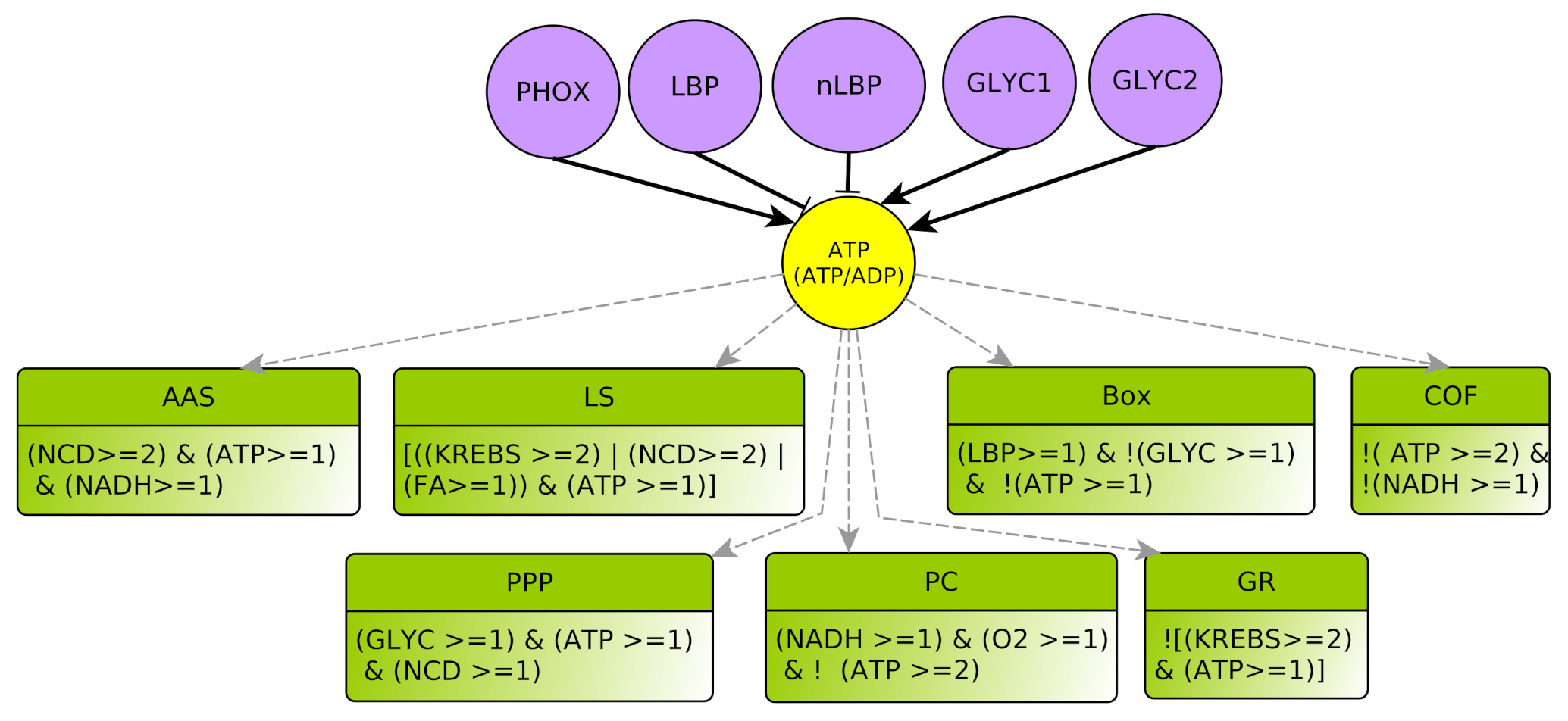
$\mathit{ATP}\in [0,2]$ represents the concentration ratio of $ATP/(ADP+AMP)$. It abstracts the energetic level for the cell. During anabolic reactions, $ATP$ is transformed into $ADP$ or $AMP$ to release energy. ADP and AMP are regenerated during glycolysis (aerobic glycolysis) or by mitochondrial respiration. Since there are shuttles between cytoplasm and mitochondria, the $ATP/(ADP+AMP)$, as a ratio, can be considered almost spatially homogeneous within the cell, even if individually the $ATP$ or $ADP$+$AMP$ level can vary greatly from mitochondria to the cytoplasm. Notice also that a high ATP value (ATP = 2) might be equally viewed as a high level of $ATP$ molecules or as a low level of $ADP$+$AMP$ molecules in the cell, and conversely for ATP = 0. Lastly, ATP = 1 represents a sort of equilibrium.

∘

$\mathit{NADH}\in [0,1]$ similarly to ATP, NADH represents the mean concentration ratio of $NADH/NA{D}^{+}$, $NADPH/NAD{P}^{+}$ as well as $FAD/FAD{H}_2$, which belong to the same electron carrier molecular group. The modeling choice of abstracting together these three different types of ratios deserves some comments. For sure, the couple $NADH/NA{D}^{+}$ is commonly used in catabolic processes whereas $NADPH/NAD{P}^{+}$ is mostly used in anabolic processes. Additionally, in Figure 3, glycolysis activates the $NADH/NA{D}^{+}$ ratio (“$+1$” plain arrow) and it does not address the same ratio as oxidative phosphorylation, which acts on $NADPH/NAD{P}^{+}$. Nevertheless, according to our very abstract level of description: (i) At the temporal resolution granularity, we consider their mean values to have the same signature as shown for example in the context of the cell cycle [25]. (ii) The thresholds between 0 and 1 are purely symbolic in the Thomas’ framework so that it is not required for the $NADH/NA{D}^{+}$ and $NADPH/NAD{P}^{+}$ thresholds to be quantitatively equal. The same reasoning applies to the $FAD/FAD{H}_2$ quotient. Therefore, we had no valuable reasons neither to distinguish between these three ratios nor to distinguish more than two different levels for the NADH targets (principle of parsimony [26]). All in all, level 0 simply represents a too low ratio to act on its targets (low $NADH$ or, equally, high $NA{D}^{+}$), contrarily to level 1.

∘

$\mathit{NCD}\in [0,2]$ represents the Nitrogen and Carbon Donors, useful to the cell and derived from amino acids. These elements are used to supply metabolic pathways such as KREBS. At level 0 NCD action is too low to undergo anabolic processes; at level 1 it can participate in the activation of the Pentose Phosphate Pathway (PPP), and at level 2 it allows the production of $\alpha$-KG through glutaminolysis even if $O_2$ is absent ($\alpha$-KG) and it also participates in amino acids and lipid synthesis (AAS and LS).

∘

$\mathit{O}\mathit{2}\in [0,1]$ represents the intracellular oxygen concentration. Once again the Thomas’ framework not being quantitative, distinguishing several thresholds for the O2 concentration can only be motivated by several targets of O2 which cannot share the same regulation thresholds. According to Figure 3, we had no valuable reason to distinguish different levels of activation for the O2 targets, so a present/absent state is sufficient in our model.

4.2.3. Metabolic pathways: GLYC, FERM, KREBS and PHOX

∘

$\mathit{GLYC}\in [0,2]$ represents glycolysis, which degrades glucose and produces pyruvate and $ATP$ (GLYC activates ATP) using ten chain reactions [27]. Three of these reactions are limiting and carried out using different enzymes, such as Phospho-Fructo-Kinase (PFK) which has a major role in glycolysis regulation. Level 0 represents glycolysis that does not produce enough intermediates, e.g., pyruvate, useful to other metabolic pathways (such as the Krebs cycle), nor any noticeable ATP. Level 1 represents a glycolytic flux sufficient to activate the related metabolic pathways (PPP). In terms of flux, PPP can be considered to be a competitor of glycolysis. However, in terms of regulation, because the variable GLYC abstracts all intermediate metabolites involved in glycolysis, GLYC is an activator of PPP (through one of its early metabolites), Krebs, etc., as well as fermentation in the absence of oxygen). Finally, level 2 represents a high level of activity where glycolysis can be considered to be over-functioning, compared to the needs of a healthy cell under optimal nutrient conditions. In such a case, glycolysis promotes the accumulation of pyruvate which in turn promotes the production of $\alpha$-KG and glycolysis also fosters the fermentation process if NADH is present, even in the presence of oxygen.

∘

$\mathit{FERM}\in [0,1]$ represents fermentation. This metabolic pathway becomes important when the oxygen supply is no longer sufficient. As $NADH$ production is the only target of FERM in the model, FERM is obviously a boolean variable.

∘

$\mathit{KREBS}\in [0,2]$ represents the TCA cycle (tricarboxylic acid cycle) or Krebs cycle. It does not represent the reverse reactions (reductive branch of the Krebs cycle) that are implicitly taken into account within multiplexes. This central metabolic cycle allows the oxidation of groups of molecules resulting from different catabolic processes (glycolysis, $\beta$-oxidation, degradation of amino acids [28]). A sufficient flow on this pathway will allow the cell to make the oxidative phosphorylation and reduce $NA{D}^{+}$ to $NADH$ (KREBS activates NADH). Its flux is dependent on the level of cellular oxygen but also on the quantity of precursors available [29]. Level 0 represents a low flux that does not allow one to noticeably obtain $NADH$. Level 1 represents a Krebs cycle flow capable of reducing $NA{D}^{+}$ to $NADH$ from basic catabolic processes (glycolysis and $\beta$-oxidation). This is the normal flow for healthy cells with an adapted supply of nutrients. At level 2 Krebs cycle is over-functioning and alarms the cell to lower catabolic processes, such as glycolysis (via GR), and promotes anabolic processes such as lipid synthesis (via LS).

∘

$\mathit{PHOX}\in [0,1]$ represents oxidative phosphorylation, a mitochondrial metabolic pathway that allows the creation of $ATP$ (PHOX activates ATP) by consuming oxygen and $NADH$ (PHOX inhibits NADH and O2). Several chemical reactions allow the reduction of an oxygen molecule into a water molecule. These steps release energy, which is used to form $ATP$. This pathway depends entirely on oxygen [30]. PHOX activates all its targets at the same level, so, it is a boolean variable.

4.2.4. Biomass: LBP and nLBP

∘

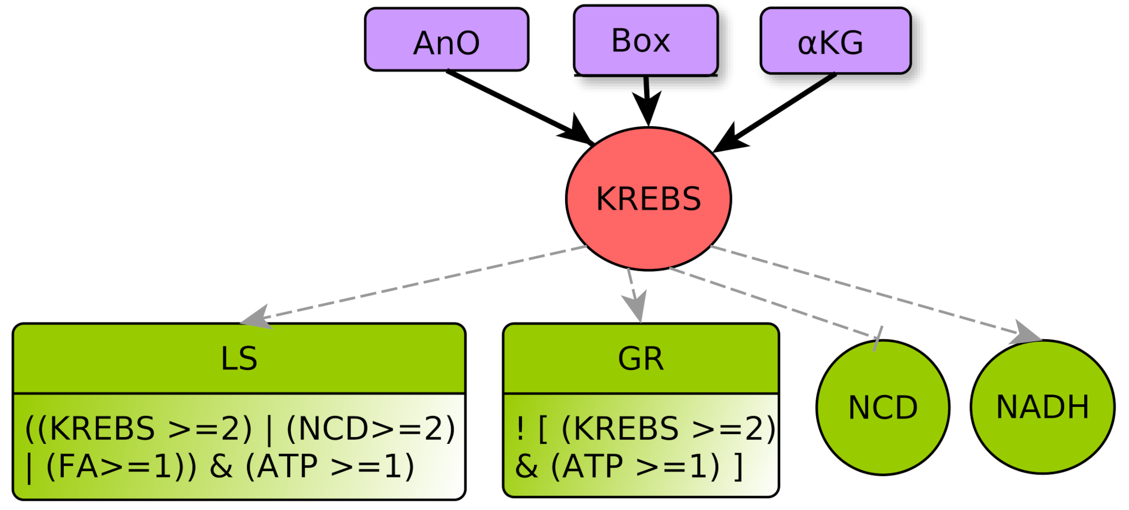
$\mathit{LBP}\mathit{ and}\mathit{ nLBP}\in [0,1]$ represents respectively the Production and storage of Lipid Biomass (all complex lipids, such as phospholipids or glycolipids) and Non-Lipidic Biomass (proteins and DNA/RNA). They are useful for component turnover and cell proliferation. Biomass production consumes energy: LBP and nLBP inhibit ATP  (Notice that lipid synthesis is in fact the process that consumes ATP, see Section 4.3.3. Technically, as LS is a multiplex, one must delegate the ATP consumption to the variable LBP. The same applies to nLBP). In addition, lipid biomass production LBP can participate in Krebs activation through Box. Whatever the kind of biomass, there is either noticeable production and storage or not, so these variables are boolean.

4.3. Multiplexes and Their Biological Meaning

In Figure 3, the grey multiplexes represent regulations of metabolic pathways whereas the red ones abstract themselves metabolic pathways. With each multiplex is associated with a logical formula, expressing the necessary conditions under which the regulation (for grey multiplexes) or the metabolic pathway (for red multiplexes) is effective. In this section, the multiplexes are sorted according to the variable they regulate and, to facilitate subsequent references, each of them is underlined and immediately followed by its associated formula.

4.3.1. Multiplexes Regulating Metabolites

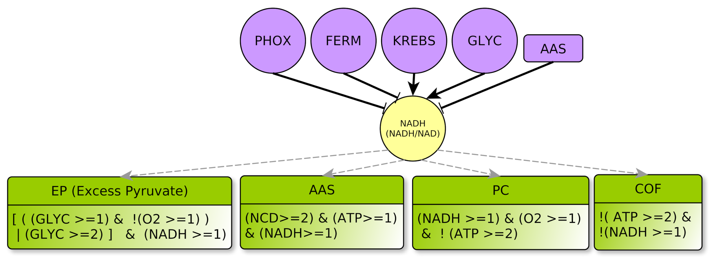
NADH Regulator

□

AAS    $(NCD⩾2)\&(ATP⩾1)\&(NADH⩾1)$ represents the processes for anabolic production of amino acids (Amino Acid Synthesis) which favor non-lipidic biomass production. They are mostly synthesized from other amino acids collected outside the cell: The multiplex AAS summarizes the necessary elements to produce new amino acids, such as nitrogen and carbon given off by the products of degradation of amino acids outside the cell $(NCD⩾2)$, a large amount of $NADH$$(NADH⩾1)$, and $ATP$ at least for some of the amino acid synthesis reactions $(ATP⩾1)$. The conjunction of these three conditions yields to the formula of this multiplex [31,32]. Moreover, $NADH$ being consumed, AAS inhibits NADH: this is encoded by the “!” (negation) on the outgoing arrow from AAS to NADH.

4.3.2. Multiplexes Regulating Pathways

GLYC Regulators

□

COF    $!(ATP⩾2)\&!(NADH⩾1)$ represents the cofactors needs to a correct course of glycolysis: $ADP$ and $NA{D}^{+}$ must not be limiting. This means that $\mathbf{ATP}<2$ and $\mathbf{NADH}<1$, as already explained in Section 4.2.2. Therefore, the COF formula properly formalizes this regulation of GLYC.

□

GR    $!\left[\right(KREBS⩾2)\&(ATP⩾1\left)\right]$ represents metabolic glycolytic flow inhibitors such as an absence of the enzyme PFK (Phospho-fructokinase) and an accumulation of citrate. Enzyme PFK of the glycolysis is allosterically inhibited by $ATP$ [33], Thus, ATP participates to inhibition of GLYC via PFK. Moreover, pyruvate (the final product of glycolysis) fuels the TCA cycle and is transformed into citrate, which, if in excess, inhibits glycolysis. Reminding that the TCA cycle is abstracted by KREBS, an excess of citrate is produced when $KREBS⩾2$, which also participates in the inhibition of glycolysis. Here, we consider that GLYC is inhibited when both conditions are satisfied, so GLYC is inhibited if $(KREBS⩾2)\&(ATP⩾1)$. The negation “!” at the beginning of the formula indicates the inhibition.

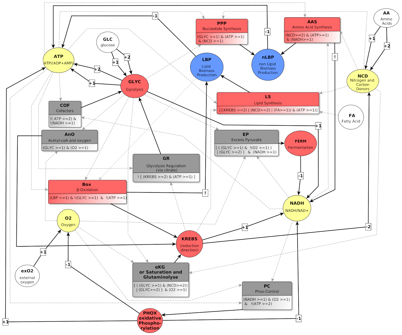
KREBS Regulators

□

AnO    $(GLYC⩾1)\&(O2⩾1)$ represents the action of AcetylcoA as main precursor of the Krebs cycle: it directly derives from pyruvate (glycolysis product) [29], which is formalized as $GLYC⩾1$. Moreover, the accumulation of Acetyl-coA coming from glycolysis activates the Krebs cycle if oxygen is present [34].

□

Box    $(LBP⩾1)\&!(GLYC⩾1)\&!(ATP⩾1)$ represents $\beta$-oxidation, the fatty acid degradation pathway. It converts fatty acids to acetyl-CoA [35]. $\beta$-oxidation can be performed when the energy level of the cell is relatively low $!(ATP⩾1)$, when the pool of stored lipids is large enough $(LBP⩾1)$ and when glycolysis is not efficient enough to produce energy $!(GLYC⩾1)$ [29]. The multiplex formula is the conjunction of these conditions.

□

$\alpha$-KG    $\left[\right(GLYC⩾1)\&(NCD⩾2\left)\right|(GLYC⩾2)]\&(O2⩾1)$ represents an accumulation of the $\alpha$-Ketoglutarate metabolite. This intermediate of a reaction of the Krebs cycle shows a significant flow only in the presence of oxygen $(O2⩾1)$ [36]. Then, the accumulation can come from a saturation issued by glycolysis with a very high flow rate $(GLYC⩾2)$. Moreover, with a lower flow rate $(GLYC⩾1)$, the transformation of glutamine to $\alpha$-KG by glutaminolysis [23,37] can accumulate, provided that the amount of amino acids in the form of nitrogen and carbon is important $(NCD⩾2)$.

FERM Regulator

□

EP    $(NADH⩾1)\&\left[\right(GLYC⩾2\left)\right|\left(\right(GLYC⩾1)\&!(O2⩾1\left)\right)]$ represents an Excess of Pyruvate, which activates the fermentation flow. Fermentation always needs $NADH$ as a cofactor $(NADH⩾1)$. Then, fermentation can be activated by an overproduction of pyruvate via glycolysis $(GLYC⩾2)$, or if glycolysis produces pyruvate at a standard rate $(GLYC⩾1)$ together with an intracellular hypoxia $!(O2⩾1)$.

PHOX Regulator

□

PC    $(NADH⩾1)\&(O2⩾1)\&!(ATP⩾2)$ represents the PHOX Control. Oxidative phosphorylation requires a sufficient supply of oxygen $(O2⩾1)$ as precursor of the chain. It also requires $NADH$$(NADH⩾1)$. Moreover, this pathway is only activated when the energy pool of the cell is not too high [38], i.e., $!(ATP⩾2)$.

4.3.3. Multiplexes Regulating Biomass

nLBP Regulators

□

PPP    $(GLYC⩾1)\&(ATP⩾1)\&(NCD⩾1)$ represents the production of nucleotides via the Pentose Phosphate Pathway that favors non-lipidic biomass production. It produces nucleotides, thus PPP activates non-lipidic biomass (nLBP). This pathway also produces $NADPH$, which is directly consumed to produce non-lipidic biomass, so that the end $NADPH$ production result is neutral for the NADH ratio. Consequently, we do not put an activation arrow from PPP to NADH in the regulation graph (contrarily to AAS). Glycolysis is required for the activation of PPP$(GLYC⩾1)$ because Glyceraldehyde-3-phosphate (G3P) is an intermediate reaction of glycolysis and the precursor of the Pentose Phosphate Pathway. In addition, for these endergonic reactions it needs a carbon input $(NCD⩾1)$ from the internalization of amino acids, as well as $ATP$$(ATP⩾1)$ [39].

The multiplex AAS (Amino-Acid Synthesis), is obviously also an activator of nLBP. It has already been described as a NADH inhibitor.

LBP regulators:

□

LS    $\left[\right((KREBS⩾2)\left|\right(NCD⩾2\left)\right|(FA⩾1))\&(ATP⩾1\left)\right]$ represents specifically the Synthesis of Lipids composed by fatty acids. Lipid creation uses energy $(ATP⩾1)$ and fatty acids can come directly from the cellular environment $(FA⩾1)$ or via the fatty acid synthesis pathway, the main precursor of which is acetyl-CoA, which is in turn provided by Krebs cycle when it is over-functioning $(KREBS⩾2)$ or by glutaminolysis directly derived from amino acids degradation $(NCD⩾2)$ [40].

The multiplex Box ($\beta$-oxidation) has already been described as a KREBS regulator which allows lipid degradation. It is consequently an inhibitor of LBP, encoded in Figure 3 through the negation sign “!” from Box to LBP.

5. Kinetic Parameters: How Local Reasoning Makes a Global Dynamics of the Mathematical Model Emerge

The interaction graph depicted in Section 4 allows the inventories and formalizes the general knowledge mentioned in Section 3. The next step to define the dynamics of our mathematical model is to guess the parameter values.

5.1. Kinetic Parameters and State Transitions

At every moment, each variable possesses a set of active resources and a complementary set of inactive resources. Let us remind that for inhibitors such as FERM on NADH, FERM becomes an active resource of NADH when it does not pass its threshold: there is an implicit multiplex with formula $(\mathit{FERM}⩾1)$ that is the actual resource of NADH. More generally, and formally, a multiplex becomes a resource of its target variable when its formula becomes true.

Figure 3 shows three particular cases: (i) the action of GLC intake on glycolysis is rather “proportional” (if the other necessary resources of glycolysis are present) than “active/inactive”; in such a case, we classically draw two actions from GLC to GLYC, with fictitious thresholds 1 and 2 and this simulates low (GLC = 0), average (GLC = 1) or high (GLC = 2) intakes; (ii) the same occurs with amino acids intake from AA to NCD; as well as (iii) the ATP production by the glycolysis GLYC. In the sequel, GLC1 denotes that GLC is at least at level 1 whereas GLC2 denotes that GLC reaches its highest level (and similarly for AA1, AA2, GLYC1 and GLYC2).

This motivates a remark: Some resource combinations are impossible, for example $K_{\mathit{GLYC},\mathbf{GLC}\mathbf{2}}$ is useless because if GLC passes threshold 2 then it also passes threshold 1, consequently only $K_{\mathit{GLYC},\mathbf{GLC}\mathbf{1}\mathbf{GLC}\mathbf{2}}$ can apply.

Once the parameter values are fixed, we consider all the possible states of all the variables of the regulation network. Our network has 7 boolean variables and 7 three-valued variables, thus it has $2^7\times 3^7$ = 279,936 states. From a given state, one can check the truth value of all the multiplex formulas. Consequently, for each variable v, we know the set $\omega$ of its resources for this state. If $K_{\mathbf{v},\omega }>v$ then v tends to grow, and it means that it is possible for v to reach its next value $v+1$: There is what we call a transition from the current state to the state where v has value $v+1$. If $K_{\mathbf{v},\omega }<v$, the transition goes from v to $v-1$, and if $K_{\mathbf{v},\omega }=v$, there is no transition related to v. Notice that there can be several variables that are attracted toward a $K_{\dots ,}$ which is different from their current value: In such a case, there are as many elementary transitions as there are such variables. We never consider transitions that modify several variables at the same time because the probability that several variables pass their thresholds exactly at the same time is null. A trajectory is consequently a succession of transitions, which we call a path. Trajectories are non-deterministic, as there are states of the network from which several variables can change their value, thus, at these steps of the path, the transition can be chosen arbitrarily.

The kinetic parameters are the key to establish the global dynamics of the mathematical model (i.e., its state transition graph) from a local biochemical knowledge encoded into the $K_{\mathbf{v},\omega }$ parameters: The value of $K_{\mathbf{v},\omega }$ is the limit value that v would reach if its set of resources $\omega$ would stay fixed forever. Let us point out that the possible values of the $K_{\mathbf{v},\omega }$ parameters are the discrete possible values of variable v. Let us remind that the values of v are separated by the thresholds of actions of v onto its targets, so that by definition, identifying the value of $K_{\mathbf{v},\omega }$ amounts to deciphering the set of targets that v can regulate when $\omega$ is its set of resources for a sufficiently long time. Let us remind that $v=m$ intrinsically means that v is active on all its targets with thresholds lower or equal to m, and inactive on all its other targets. Consequently, the thought experiment amounts to foresee on which v is active after its stabilization.

Some of these thought experiments can be inconclusive, and of course the state transition graph is far too huge to be manually studied, or even properly visualized. In such a case, we keep all possible values of these parameters compatible with the thought experiments and we will see in Section 7 how biological knowledge about the global behavior of the system (Section 6) can help us to automatically select those of biological interest. Let us first inventory the successful thought experiments.

5.2. Local Identification of Parameters for Metabolic Regulations

Owing to the coarse-grained level of abstraction of our model, where variables and multiplexes mostly refer to classical biochemical markers, we take benefit of a long history of accumulated biochemical knowledge [41,42,43]. Elucidated parameter values are summarized in Table 1.

GLYC Parameters

Properly conducting parameter identifications for a given variable requires to have in mind all possible resources and all targets of the variable. Figure 4 focuses on this information for the variable GLYC: It is potentially active from its level 1 for all its targets, but, depending on external conditions, level 2 can be required. More precisely level 2 of GLYC  is necessary to act on three targets:

• EP if $\mathit{O}\mathit{2}=1$ and $\mathit{NADH}⩾1$,
• $\alpha$KG if $\mathit{NCD}<2$ and $\mathit{O}\mathit{2}=1$,
• over-activation of ATP (compared to “simple” activation performed at level 1).

In the first phase of the reasoning, we put aside parameters with inconsistent resources. We already remarked that GLC2 implies GLC1 as resource, thus $K_{\mathit{GLYC},\mathbf{GLC}\mathbf{2}}$, $K_{\mathit{GLYC},\mathbf{COF}\mathbf{GLC}\mathbf{2}}$, $K_{\mathit{GLYC},\mathbf{COF}\mathbf{GLC}\mathbf{2}\mathbf{GR}}$ and $K_{\mathit{GLYC},\mathbf{GLYC}\mathbf{2}\mathbf{GR}}$ reflect inconsistent sets of resources and therefore have not to be instantiated. Therefore, it remains $2^4-4=12$ GLYC parameters to estimate.

The second phase of the reasoning treats easy cases, mostly when the variable under consideration is attracted toward 0, by lack of resources. Here GLC and COF (cofactors) are prerequisites for glycolysis: if one of them is missing, the glycolysis cannot occur, and it becomes unable to act on its targets. It implies that 8 parameters are equal to 0: $K_{\mathit{GLYC},}$, $K_{\mathit{GLYC},\mathbf{GLC}\mathbf{1}}$, $K_{\mathit{GLYC},\mathbf{COF}}$, $K_{\mathit{GLYC},\mathbf{GR}}$, $K_{\mathit{GLYC},\mathbf{GLC}\mathbf{1}\mathbf{GLC}\mathbf{2}}$, $K_{\mathit{GLYC},\mathbf{GLC}\mathbf{1}\mathbf{GR}}$, $K_{\mathit{GLYC},\mathbf{COF}\mathbf{GR}}$ and $K_{\mathit{GLYC},\mathbf{GLC}\mathbf{1}\mathbf{GLC}\mathbf{2}\mathbf{GR}}$.

Other usually easy cases arise when the variable under consideration takes benefit of all its resources, or when no inhibitor act on it (thus, when all inhibitors are resources of the variable). Here, GR reflects an inhibition of glycolysis by KREBS and ATP (that make PFK unavailable to glycolysis). Therefore, when GR is a resource of GLYC, if cofactors and glucose are present, then the greater the level of glucose, the greater the level of glycolysis:

• When $\mathit{GLC}=2$ the functioning of glycolysis will reach a level that is sufficient to activate EP even if $\mathit{O}\mathit{2}=1$ and $\mathit{NADH}⩾1$, as well as $\alpha$KG if $\mathit{NCD}<2$ and $\mathit{O}\mathit{2}=1$. Thus $K_{\mathit{GLYC},\mathbf{COF}\mathbf{GLC}\mathbf{1}\mathbf{GLC}\mathbf{2}\mathbf{GR}}=2$.
• When $\mathit{GLC}=1$ the functioning of glycolysis will allow the activation of its targets (if the other conditions are satisfied), but neither EP if $\mathit{O}\mathit{2}=1$ and $\mathit{NADH}⩾1$, nor $\alpha$KG if $\mathit{NCD}<2$ and $\mathit{O}\mathit{2}=1$. Thus $K_{\mathit{GLYC},\mathbf{COF}\mathbf{GLC}\mathbf{1}\mathbf{GR}}=1$.

The last phase of the reasoning is to try to identify parameters with intermediate sets of resources. Here two parameter values remain so far unknown: $K_{\mathit{GLYC},\mathbf{COF}\mathbf{GLC}\mathbf{1}\mathbf{GLC}\mathbf{2}}$ and $K_{\mathit{GLYC},\mathbf{COF}\mathbf{GLC}\mathbf{1}}$. In both cases, nutrient (GLC) and cofactors (COF) are present, and GR acts as an inhibitor that will reduce the effectiveness of glycolysis. In fact, the inhibition via GR, even in the presence of high glucose, stops the “suractivation” of ATP and EP when $\mathit{O}\mathit{2}=1$ and $\mathit{NADH}⩾1$, thus $K_{\mathit{GLYC},\mathbf{COF}\mathbf{GLC}\mathbf{1}\mathbf{GLC}\mathbf{2}}=1$. With the normal presence of glucose, GR is even strong enough to stop the activation of all downstream processes through glycolysis, thus $K_{\mathit{GLYC},\mathbf{COF}\mathbf{GLC}\mathbf{1}}=0$.

In the remainder of this section, this methodology in four phases is the same for all other parameters. In some cases, the abstraction of biological knowledge can be difficult and we take care to make all our interpretation choices explicit. They can be regarded as sensible assumptions in the context of our generic eukaryote metabolism regulation study, and these assumptions might be reevaluated if the model is used to deal with new questions or more specialized cells.

KREBS Parameters

KREBS has a dual role depending on the cell’s milieu. At level 1, KREBS is a provider of NADH to normal functioning of the cell. At level 2 KREBS is overspreading and alarms glycolysis (through the GR inhibition) to lower the production of pyruvate and to lower the intake of elements coming from amino acids to break Krebs turnover. At level 2 KREBS also provokes lipid production. Therefore, KREBS is an inhibitor of GLYC and NCD, and an activator of lipid synthesis LS. See Figure 5.

Resources of KREBS are: BOX through fatty acid degradation, $\alpha$KG coming from glutaminolysis, and AnO because acetyl-CoA is derived from pyruvate, the final product of glycolysis. Thus there are $2^3=8$ parameters to identify for KREBS.

Useless parameters (please refer to multiplex formulas in Figure 3): The $\alpha$KG formula implies the one of AnO, reflecting the fact that both $\alpha$KG and AnO came from glycolysis. Moreover, the BOX formula implies GLYC=0, and thus contradicts the ones of $\alpha$KG and AnO. Therefore, $K_{\mathit{KREBS},\alpha \mathbf{KG}}$ , $K_{\mathit{KREBS},\mathbf{BOX}\alpha \mathbf{KG}}$ , $K_{\mathit{KREBS},\mathbf{AnO}\mathbf{BOX}\alpha \mathbf{KG}}$ and $K_{\mathit{KREBS},\mathbf{AnO}\mathbf{BOX}}$ are useless.

Lack of resources: When none of the three potential resources of KREBS is available, it cannot activate any downstream target. Thus $K_{\mathit{KREBS},}=0$.

Full resources: When KREBS has the full support of $\alpha$KG and AnO, it will give an alarm to catabolic processes as glycolysis or degradation of amino acids intake (NCD) to avoid overproduction of energy and it also promotes anabolic processes. Thus $K_{\mathit{KREBS},\mathbf{AnO}\alpha \mathbf{KG}}=2$.

Intermediate sets of resources: In the presence of normal intake of Acetyl-CoA through glycolysis (AnO), KREBS produces $NADH$ without alarming the cell. Thus, $K_{\mathit{KREBS},\mathbf{AnO}}=1$, and for the same reason $K_{\mathit{KREBS},\mathbf{BOX}}=1$.

FERM and PHOX Parameters

Fermentation and oxidative phosphorylation are easy cases because they have only two possible values (boolean variables) and exactly one resource each (respectively EP that denotes an excess of pyruvate, and PC that denotes the PHOX control, see Figure 6). In both cases, if the resource is absent, then FERM or PHOX will become unable to act on their targets, thus $K_{\mathit{FERM},}=0$ and $K_{\mathit{PHOX},}=0$. Conversely, if the resource is present, they will become able to act on their targets, thus $K_{\mathit{FERM},\mathbf{EP}}=1$ and $K_{\mathit{PHOX},\mathbf{PC}}=1$.

nLBP Parameters

The non-lipidic biomass production variable nLBP is boolean, acting on ATP consumption (see Figure 7). It has 2 possible resources: PPP and AAS, whose combinations are all satisfiable, meaning that each of the 4 conjunctions of their formulas or their negations are true for at least one state of the network. Therefore, all 4 parameters are useful.

If neither nucleotide synthesis nor amino acid synthesis occur (lack of resources), then the production of non-lipidic biomass will stop, thus $K_{\mathit{nLBP},}=0$. Conversely, in the presence of PPP or in the presence of AAS, the non-lipidic biomass production becomes sufficiently activated to consume ATP, thus $K_{\mathit{nLBP},\mathbf{PPP}}=K_{\mathit{nLBP},\mathbf{AAS}}=K_{\mathit{nLBP},\mathbf{AAS}\mathbf{PPP}}=1$.

LBP Parameters

The complex lipidic production variable LBP is also boolean and it consumes ATP and favors Box concomitantly. Possible resources of LBP are lipid synthesis LS and Box, and this makes the thought experiments particularly subtle: even when Box is supposed inactive forever as a resource of LBP, one must consider fully independently the possible action of LBP on Box as a target. In other words, one must consider that Box as a resource is different from Box as a target. More generally, these thought experiments only take into account the local biochemical behavior without considering its effect on the whole network (see Figure 8).

All combinations of LS and Box are satisfiable, so that the 4 parameters are useful. Without lipidic synthesis LBP lacks resources, thus $K_{\mathit{LBP},}=K_{\mathit{LBP},\mathbf{BOX}}=0$. Conversely, with lipidic synthesis, even if Box inhibits LBP, lipid biomass as precursor activates its degradation and consumes ATP, thus $K_{\mathit{LB},\mathbf{LS}}=1$ and a fortiori $K_{\mathit{LBP},\mathbf{LS}\mathbf{BOX}}=1$.

NCD Parameters

NCD is a provider of nitrogen and carbon coming from amino acids: In our model, AA is the input provider of NCD at two different levels, and KREBS inhibits NCD. Thus, 8 kinetic parameters drive NCD. At level 1, NCD allows the creation of nucleotides and DNA by providing nitrogen via PPP. At level 2, it allows the creation of $\alpha$KG via glutaminolysis, as well as amino acids via the amino acids synthesis pathway AAS, and lipid synthesis LS by providing nitrogen and carbon. See Figure 9.

Useless parameters come from the fact that AA at level 2 implies that AA at level 1 is also a resource of NCD, as already explained, thus $K_{\mathit{NCD},\mathbf{AA}\mathbf{2}}$ and $K_{\mathit{NCD},\mathbf{AA}\mathbf{2}\mathbf{KREBS}}$ are useless.

Without inhibitor that is when the KREBS level does not reach 2: NCD is fully under the control of amino acid intake AA. If AA=0, then without input of amino acids, no nitrogen is provided and none of the target processes downstream of NCD can be activated ($K_{\mathit{NCD},\mathbf{KREBS}}=0$). If AA=1, there is enough production of nucleotide via the pathway PPP but not enough production of nitrogen and carbon to be active on amino acid AAS or lipid LS synthesis, as well as $\alpha$KG, thus $K_{\mathit{NCD},\mathbf{AA}\mathbf{1}\mathbf{KREBS}}=1$. Lastly if AA = 2, then NCD becomes active on AAS, LS and $\alpha$KG, thus $K_{\mathit{NCD},\mathbf{AA}\mathbf{1}\mathbf{AA}\mathbf{2}\mathbf{KREBS}}=2$.

With inhibitor: We established previously that $K_{\mathit{NCD},\mathbf{KREBS}}=0$, so a fortiori $K_{\mathit{NCD},}=0$. More generally, with respect to the thresholds of NCD to be active on PPP, $\alpha$KG, AAS and LS, we consider that the inhibition of KREBS will lower down the production speed of nitrogen and carbon, but this will not decrease the value toward which KREBS asymptotically tends (technically because there is no degradation of nitrogen and carbon as such). Therefore, $K_{\mathit{NCD},\mathbf{AA}\mathbf{1}}=K_{\mathit{NCD},\mathbf{AA}\mathbf{1}\mathit{KREBS}}=1$ and $K_{\mathit{NCD},\mathbf{AA}\mathbf{1}\mathbf{AA}\mathbf{2}}=K_{\mathit{NCD},\mathbf{AA}\mathbf{1}\mathbf{AA}\mathbf{2}\mathbf{KREBS}}=2$.

O2 Parameters

The O2 activator exO2 (oxygen supply) and O2 inhibitor PHOX (oxidative phosphorylation which consumes oxygen) are independent of each other (see Figure 10), thus the 4 kinetic parameters for O2 are useful. All the targets of O2, AnO, $\alpha$KG, EP and PC share the same threshold: O2 is simply present or absent.

Of course, without external oxygen supply, O2 lack of resources, thus $K_{\mathit{O}\mathit{2},}=K_{\mathit{O}\mathit{2},\mathbf{PHOX}}=0$. Conversely, external oxygen constantly renews O2, so that $K_{\mathit{O}\mathit{2},\mathbf{exO}\mathbf{2}}=K_{\mathit{O}\mathit{2},\mathbf{exO}\mathbf{2}\mathbf{PHOX}}=1$.

NADH Parameters

Let us remind that NADH stands for the quotient $NAD\left(P\right)H/NAD{\left(P\right)}^{+}$, thus NADH = 1 equally means presence of $NAD\left(P\right)H$ or lack of $NAD{\left(P\right)}^{+}$, and NADH = 0 equally means presence of $NAD{\left(P\right)}^{+}$ or lack of $NAD\left(P\right)H$. It acts as activator for phosphorylation (PHOX via PC when O2 is present), for fermentation (FERM via EP when there is hypoxia or when glycolysis produces an excess of pyruvate) and for amino acid synthesis (when ATP and NCD are sufficiently present). It also acts as inhibitor for glycolysis (GLYC via COF).

NADH has 2 source providers: KREBS and GLYC, and 3 consumers: PHOX, FERM and AAS, see Figure 11. All combinations of these 5 potential resources are satisfiable, leading to 32 parameters to identify.

Lack of resources: When neither KREBS nor GLYC is present NADH will obviously not activate its targets, thus $K_{\mathit{NADH},}=K_{\mathit{NADH},\mathbf{FERM}}=K_{\mathit{NADH},\mathbf{PHOX}}=K_{\mathit{NADH},\mathbf{AAS}}=K_{\mathit{NADH},\mathbf{FERM}\mathbf{PHOX}}=K_{\mathit{NADH},\mathbf{FERM}\mathbf{AAS}}=K_{\mathit{NADH},\mathbf{AAS}\mathbf{PHOX}}=K_{\mathit{NADH},\mathbf{FERM}\mathbf{AAS}\mathbf{PHOX}}=0$.

No inhibitor and at least an activator: No $NAD\left(P\right)H$ is consumed and no $NAD{\left(P\right)}^{+}$ is produced, so, even if the activator is weak, its long-term action will increase the NADH quotient and thus downstream targets will finally be activated. Thus, $K_{\mathit{NADH},\mathbf{GLYC}\mathbf{FERM}\mathbf{AAS}\mathbf{PHOX}}=K_{\mathit{NADH},\mathbf{KREBS}\mathbf{FERM}\mathbf{AAS}\mathbf{PHOX}}=K_{\mathit{NADH},\mathbf{GLYC}\mathbf{KREBS}\mathbf{FERM}\mathbf{AAS}\mathbf{PHOX}}=1$.

Intermediate sets of resources: 21 parameter values remain to be identified for NADH, and we can set most of them owing to two hypotheses that seem sensible within our context:

• In the cell, PHOX is the principal consumer of NADH, KREBS is its principal producer, and the metabolic processes they abstract are nested, therefore they balance on a long-term basis.
• GLYC is a weak producer of NADH, FERM is an average consumer, and AAS is a weak consumer (but we do not know if GLYC and AAS balance on a long-term basis).

The first hypothesis, once translated in terms of resources, implies that $K_{\mathit{NADH},\mathbf{FERM}\mathbf{KREBS}\mathbf{AAS}}=0$ as KREBS and PHOX are putted aside (they are in balance), so the situation is similar to no provider, and there is no remaining inhibitor nor activators. From the second hypothesis, it comes $K_{\mathit{NADH},\mathbf{GLYC}\mathbf{AAS}\mathbf{PHOX}}=0$ because, here, the only producer GLYC is weak and the average consumer FERM is on. Taking into account the balance between KREBS and PHOX, the second hypothesis also implies $K_{\mathit{NADH},\mathbf{GLYC}\mathbf{KREBS}\mathbf{AAS}}=0$ for the same reason. We can also deduce that $K_{\mathit{NADH},\mathbf{FERM}\mathbf{GLYC}\mathbf{AAS}}=0$, as GLYC is here the only activator and the principal inhibitor PHOX is on. Therefore, the hypotheses require 4 parameter values to 0, and, a fortiori with less resources, we deduce 8 more parameter values: $K_{\mathit{NADH},\mathbf{GLYC}\mathbf{KREBS}}=K_{\mathit{NADH},\mathbf{FERM}\mathbf{KREBS}}=K_{\mathit{NADH},\mathbf{KREBS}\mathbf{AAS}}=K_{\mathit{NADH},\mathbf{GLYC}\mathbf{AAS}}=K_{\mathit{NADH},\mathbf{GLYC}\mathbf{PHOX}}=K_{\mathit{NADH},\mathbf{FERM}\mathit{GLYC}}=K_{\mathit{NADH},\mathbf{KREBS}}=K_{\mathit{NADH},\mathbf{GLYC}}=0$.

Conversely, the hypotheses imply $K_{\mathit{NADH},\mathbf{FERM}\mathbf{GLYC}\mathbf{KREBS}\mathbf{AAS}}=1$ because PHOX is in equilibrium with KREBS, there is no other inhibitor, and consequently the GLYC activation makes the difference. We also obtain $K_{\mathit{NADH},\mathbf{KREBS}\mathbf{PHOX}}=1$ (where KREBS is the only activator and AAS and FERM are inhibitors) because the principal producer KREBS, not balanced by the PHOX inhibition, contributes to the $NAD\left(P\right)H/NAD{\left(P\right)}^{+}$ quotient more than FERM and AAS together, which are at most average consumers. Then, a fortiori with more resources, we deduce $K_{\mathit{NADH},\mathbf{KREBS}\mathbf{FERM}\mathbf{PHOX}}=K_{\mathit{NADH},\mathbf{KREBS}\mathbf{AAS}\mathbf{PHOX}}=K_{\mathit{NADH},\mathbf{GLYC}\mathbf{KREBS}\mathbf{PHOX}}=K_{\mathit{NADH},\mathbf{FERM}\mathbf{GLYC}\mathbf{KREBS}\mathbf{PHOX}}=K_{\mathit{NADH},\mathbf{GLYC}\mathbf{KREBS}\mathbf{AAS}\mathbf{PHOX}}=1$

So far, two parameters out of 32 have not been found: $K_{\mathit{NADH},\mathbf{FERM}\mathbf{GLYC}\mathbf{KREBS}}$ and $K_{\mathit{NADH},\mathbf{FERM}\mathbf{GLYC}\mathbf{PHOX}}$, for which the only producer is GLYC and the consumer is AAS (for the first parameter, considering the KREBS/PHOX balance simplification from the first hypothesis). GLYC and AAS are both weak but we cannot figure out a sensible third hypothesis (that would not be too arbitrary with respect to our general context) to assert a proper comparison. Therefore, let us leave those parameters unknown and Section 7 will handle the question properly.

ATP Parameters

ATP stands for the quotient $ATP/ADP$, with two activity thresholds. At level 1 it participates in the amino acid, the nucleotide and the lipid syntheses (AAS, PPP and LS), it inhibits $\beta$-oxidation BOX, and it down-regulates glycolysis when KREBS = 2 via GR. At level 2, it additionally inhibits oxidative phosphorylation through PC and down-regulates glycolysis once more via COF. See in Figure 12.

ATP has 3 providers: two levels of glycolysis (GLYC1 and GLYC2) as well as oxidative phosphorylation (PHOX). It has 2 consumers: LBP and nLBP (biomass productions). Of course, the resource GLYC2 implies GLYC1, thus there are 8 useless parameters: $K_{\mathit{ATP},\mathbf{GLYC}\mathbf{2}}$, $K_{\mathit{ATP},\mathbf{GLYC}\mathbf{2}\mathbf{PHOX}}$, $K_{\mathit{ATP},\mathbf{GLYC}\mathbf{2}\mathbf{LBP}}$, $K_{\mathit{ATP},\mathbf{GLYC}\mathbf{2}\mathbf{nLBP}}$, $K_{\mathit{ATP},\mathbf{GLYC}\mathbf{2}\mathbf{PHOX}\mathbf{LBP}}$, $K_{\mathit{ATP},\mathbf{GLYC}\mathbf{2}\mathbf{PHOX}\mathbf{nLBP}}$, $K_{\mathit{ATP},\mathbf{GLYC}\mathbf{2}\mathbf{LBP}\mathbf{nLBP}}$ and $K_{\mathit{ATP},\mathbf{GLYC}\mathbf{2}\mathbf{PHOX}\mathbf{LBP}\mathbf{nLBP}}$. It remains consequently 24 parameters to identify.

Lack of resources: When neither PHOX nor GLYC is present ATP will finally not be able to activate its targets, thus $K_{\mathit{ATP},\mathbf{LBP}\mathbf{nLBP}}=K_{\mathit{ATP},\mathbf{LBP}}=K_{\mathit{ATP},\mathbf{nLBP}}=K_{\mathit{ATP},}=0$.

No inhibitor: without consumption of ATP, the presence of any ATP provider will make ATP tend to its higher value where it is able to act on all its targets. Thus, $K_{\mathit{ATP},\mathbf{LBP}\mathbf{nLBP}\mathbf{PHOX}}=K_{\mathit{ATP},\mathbf{GLYC}\mathbf{1}\mathbf{LBP}\mathbf{nLBP}\mathbf{PHOX}}=K_{\mathit{ATP},\mathbf{GLYC}\mathbf{1}\mathbf{GLYC}\mathbf{2}\mathbf{LBP}\mathbf{nLBP}\mathbf{PHOX}}=K_{\mathit{ATP},\mathbf{GLYC}\mathbf{1}\mathbf{LBP}\mathbf{nLBP}}=$$K_{\mathit{ATP},\mathbf{GLYC}\mathbf{1}\mathbf{GLYC}\mathbf{2}{LBP}\mathbf{nLBP}}=2$.

Intermediate sets of resources: let us first consider when LBP and nLBP both consume ATP (i.e., when they are not resources). If PHOX is present as an activator, it produces enough ATP to activate anabolic pathways such as PPP or AAS, and to inhibit $\beta$-oxidation, but the production will not be powerful enough to ring overproduction retro-controls via PC or COF. The same arises if glycolysis at level 2 is an activator. Indeed, in terms of metabolic pathways, the energetic balance between oxidative phosphorylation and glycolysis is widely in favor of phosphorylation, except when the glycolysis is over-speeding. For this reason, PHOX and GLYC at level 2 will tend to activate the same targets downstream ATP when biomass production consumes ATP. Thus, $K_{\mathit{ATP},\mathbf{PHOX}}=K_{\mathit{ATP},\mathbf{GLYC}\mathbf{1}\mathbf{PHOX}}=K_{\mathit{ATP},\mathbf{GLYC}\mathbf{1}\mathbf{GLYC}\mathbf{2}}=K_{\mathit{ATP},\mathbf{GLYC}\mathbf{1}\mathbf{GLYC}\mathbf{2}\mathbf{PHOX}}=1$. When GLYC=1 is the only ATP producer, glycolysis is not over-speeding and there is not enough ATP produced against biomass production consumers. Thus $K_{\mathit{ATP},\mathbf{GLYC}\mathbf{1}}=0$.

So far 10 ATP parameters remain to be identified: those where at least one ATP producer is present and exactly one of the two consumers nLBP or LBP is in action. To go further, the following hypothesis seems sensible: When lipidic biomass production is on, the ATP consumption of non-lipidic biomass production will not change the limit value toward which ATP is attracted. This offers 5 more parameter values: $K_{\mathit{ATP},\mathbf{nLBP}\mathbf{PHOX}}=K_{\mathit{ATP},\mathbf{GLYC}\mathbf{1}\mathbf{nLBP}\mathbf{PHOX}}=K_{\mathit{ATP},\mathbf{GLYC}\mathbf{1}\mathbf{GLYC}\mathbf{2}\mathbf{nLBP}}=K_{\mathit{ATP},\mathbf{GLYC}\mathbf{1}\mathbf{GLYC}\mathbf{2}\mathbf{nLBP}\mathbf{PHOX}}=1$ and $K_{\mathit{ATP},\mathbf{GLYC}\mathbf{1}\mathbf{nLBP}}=0$.

Just as we did for 2 NADH parameters, let us leave the 5 remaining ATP parameters unknown and Section 7 will handle the question properly.

Summarizing this section, for each possible set of values of the 7 remaining parameters, Thomas’ modeling framework defines a unique mathematical dynamics of the system. The main question is now to verify if one of these possible dynamics is biologically compatible with available biological knowledge about the global behavior of the cell. This is the purpose of Section 6, formalizing this biological knowledge, and Section 7 that makes the bridge between the formalized biological knowledge and mathematical dynamics using automated formal proofs.

6. Validation Matrix: Encoding Global Biological Knowledge Using Temporal Logic

In this section, we carefully ignore the local knowledge used in Section 5. Once the set of variables in the model has been established (Section 4), we can list available knowledge about its global phenotypes in terms of these variables, comprising both anabolic and catabolic functioning and Warburg/Crabtree effects. We formalize them into a table, called de validation matrix (Table 2), where each row represents an environmental condition under which some properties have been observed, and each column represents a marker.

• The environmental conditions are defined by the four environmental variables described above (Section 4.2): presence of glucose, availability of fatty acids, etc.
• and the markers of the global functioning are the regulated variables: biomass production, the activity level of the Krebs cycle, concentration ratio $NAD\left(P\right)H/NAD{\left(P\right)}^{+}$, etc.

At the crossing between a row and a column, we describe which kind of behavior the marker must exhibit, if well-established from biological or biochemical knowledge. This behavior is formalized using a temporal logic formula in the corresponding box of the table.

The result of this section will be the validation matrix of Table 2. It formalizes and synthesizes the commonly accepted knowledge about the global behaviors of generic cell metabolism in different contexts. When we doubt biological consensus, the matrix exhibits a grey box, so that our model remains open to different types of cells leading to a sort of “generic model”. Unless specified otherwise we extract this consensus knowledge from manuals such as [41,42,43].

6.1. A Logic for Asymptotic Behaviors

Logical formulas similar to the ones carried by multiplexes are able to formalize instant properties about a given state of the system. When it comes to temporal properties, at the level of sub-cellular behavior, most of the phenomena are stochastic consequently not deterministic. Thus, simple logical formulas are not enough to capture the evolution of a regulation network along time: a temporal logic is needed. Moreover, to be able to capture cell phenotypes, one cannot be satisfied with a pure temporal logic: we need to address long time convergence, which rely on asymptotic behavior.

Computation Tree Logic [16] (CTL) has proved its effectiveness for biological regulation networks [6,44]. Its tree-like representation of time allows for an indeterminism on the possible behaviors: As biological systems are not deterministic, from a given current state of the regulation network, it is possible to observe different traces with different successive observations. CTL can easily express that a property can be true only within certain paths, using the E quantifier that means there Exists a path such that… It can also easily express that a property is true within All possible paths, using the A quantifier. Moreover, CTL also offers 4 so-called modalities about time passing along a given path: X stands for the neXt state after the current state, F stands for some Future state (without specifying when it happens), G stands for all future events (Globally), and U allows one to specify that something is true Until another property becomes true.

More precisely each temporal connective is made of two letters: the first one is the quantifier (A or E) and the second one is the modality (X, F, G or U). For example, “$EX(\mathit{O}\mathit{2}=0)$” stands for “in the current state, it is possible that at the next state, the oxygen reaches its lower level”. Similarly, “$AG(\mathit{AA}=0)\Rightarrow AF\left(AG\right(\mathit{NCD}=0\left)\right)$” means that “from any context where there is never external Amino Acid intake ($AG(\mathit{AA}=0)$), all possible paths lead to a state ($AF$) where Nitrogen and Carbon Donors will stay low forever ($AG(\mathit{NCD}=0)$).

With such a temporal logic, it becomes possible to formally express global knowledge about biological phenomena: epigenetic phenomena, homeostasis, (non-)reachability of certain states, events that always happen after others (but not necessarily right after), etc. Nevertheless CTL, as such, is unable to capture asymptotic behaviors, due to the existence of “unfair” cyclic paths. For example, “$AG(\mathit{AA}=0)\Rightarrow AF\left(AG\right(\mathit{NCD}=0\left)\right)$” may become false in pure CTL. This is because there exists an infinite artefactual path where only ATP or NADH oscillate, and where NCD is never updated. At our level of abstraction, such a path is highly improbable because it is unfair with respect to the lowering of NCD. This leads us to adopt the “fair-paths” semantics: A formula containing the quantifier A is evaluated on all paths except the non “fair” ones: For a path to be taken into account, it is necessary that if a state is visited an infinite number of times, none of its outgoing events can be neglected forever. This variant of CTL, where the quantifiers A and E do not consider unfair paths, is called fair-path CTL.

Fortunately, there is a systematic translation algorithm from fair-path CTL formulas to equivalent CTL formulas [45], so that we take benefit of all the CTL software tools. Indeed, once a temporal property has been written in CTL, one can automatically, and very efficiently, check whether a model satisfies the specified property using a so-called model checker such as NuSMV [46], which will be intensively used in Section 7.

In the sequel, we use fair-path CTL for representing phenotypic behaviors, and two patterns of formulas are introduced for readability:

• The pattern “osc” depicts oscillations of the considered marker. If one knows the highest and lowest boundaries of this oscillation, one can specify these boundaries, e.g., “osc(1,2)” indicates that the variable under consideration oscillates between 1 and 2. However, if such boundaries are unknown, “osc” simply specifies that the oscillation takes place without any constraints on the boundaries.
• The pattern “td(n)” specifies that the variable under consideration tends toward the value n. It specifies that the marker tends toward a global equilibrium.

Lastly, in Table 2, the logical negation “!” indicates that a behavior (specified by one of the previously described patterns) is not valid with respect to biological knowledge.

6.2. Validation Matrix for the Regulation of Metabolism

The validation matrix given in Table 2 lists all known behaviors (phenotypes) about the metabolism in the context of the Warburg/Crabtree effect, according to different environmental contexts such as nutrient conditions (Section 4.2.1). Each row represents such a context, i.e., a setting of environmental variables (white variables in Figure 3). There are 36 possible contexts, so the validation matrix contains 36 lines. Each column represents a biologically interpretable variable, possibly experimentally observable, which we call “markers” by language abuse. In addition to the 4 environmental variables (light grey columns) that define the environmental contexts, the 10 systemic variables are considered to be markers (yellow, red and blue circles in Figure 3). Table 2 leaves the NCD column implicit because its asymptotic behavior is under the control of the level of AA, which imposes to NCD the value toward which it tends, so the NCD column would be a copy (up to the “td()” pattern) of the AA column. Table 2 should be regarded as a $36\times 9$ matrix of fair-path CTL formulas that formalize the known behaviors of these markers (with a tenth implicit column). When no general knowledge about the behavior of a given marker in a given context is available, the corresponding box remains empty (dark grey).

A valid qualitative model must at least exhibit all the behaviors of this validation matrix: the parameter settings of Section 5.2 will be confronted against it. It is important to note that we only use fair-path CTL, and consequently, each specified behavior in the validation matrix must be understood as asymptotic.

Section 6.2.1, Section 6.2.2 and Section 6.2.3 below list the 36 environmental contexts of the validation matrix. Sometimes two contexts are glued together in the same line, e.g., the contexts 2 and 3, because the general knowledge about the marker behaviors in these two contexts is identical. For each line of Table 2 we justify the fair-path CTL statement of each marker behavior, according to general biological knowledge. We graphically use “⇝” followed by the line number to introduce each line description.

Unless otherwise stated, “general knowledge” refers to biochemistry books such as [41,42,43].

6.2.1. Without Lipid Intake and without Oxygen Supply

⇝

1—FA = 0, exO2 = 0, GLC = 0, AA = 0: Leads to cell death. Cells require sufficient nutrients to supply the metabolic demands for cell growth and division. When all inputs are absent, no production of any component of the cell is possible and thus each variable tends toward 0. This would lead to cell death.

⇝

2 & 3—FA = 0, exO2 = 0, GLC = 0, AA = (1 or 2): The cell has only amino acids as nutrient supply. There is no general knowledge to assert whether amino acid intake alone can sustain carbon-dependent metabolic activity of the cell even if there are culture media without glucose for certain cancer cell lines [20,22]. Thus, we consider that cell fate is unknown, except that with no input of oxygen, the cell becomes in hypoxia and O2 tends toward 0.

⇝

4—FA = 0, exO2 = 0, GLC = 1, AA = 0: Leads to aerobic glycolysis. Without oxygen and with glucose as a unique carbon source, mitochondrial respiration cannot occur and the only metabolic pathway is fermentation. Even if ATP is consumed for cell maintenance, it at least does not tend to zero as the cell can survive with only glucose. $NA{D}^{+}$ is consumed during glycolysis and regenerated during fermentation; Glucose intake allows the production of lactate, which reduces $NADH$ to $NA{D}^{+}$, which is recycled back to $NADH$ by glycolysis, so NADH oscillates. By the absence of oxygen supply, O2 tends toward 0 and mitochondrial activity is shunted, so PHOX tends toward 0. Lastly, GLC=1 denotes a glucose intake insufficient to make glycolysis reach its higher rate, so GLYC oscillates between 0 and 1.

⇝

5—FA = 0, exO2 = 0, GLC = 1, AA = 1: Leads to aerobic glycolysis. An additional supply of amino acids allows for non-lipidic biomass production, so nLBP does not tend toward 0. This anabolic process consumes $ATP$, and as it is also produced, $ATP$ should oscillate. In addition, as in ⇝4, the cell is in an anaerobic process, and cytosolic metabolism and mitochondrial activity act similarly on the other markers.

⇝

6—FA = 0, exO2 = 0, GLC = 1, AA = 2: Leads to aerobic glycolysis. A huge supply on amino acids favors the reductive phase of Krebs to provide precursors for lipid synthesis, so LBP does not tend toward 0. The metabolic processes are the same as ⇝5, except that a large intake of amino acids activates glutaminolysis. It creates $\alpha$-ketoglutarate that can be converted with the reductive Krebs cycle in pyruvate. This accumulation of pyruvate could also be due to high activity of GLYC, therefore GLYC could sometimes reach its highest level. Thus, we prefer to relax its oscillatory behavior (“osc” without knowledge of the boundaries instead of “osc (0,1)”).

⇝

7—FA = 0, exO2 = 0, GLC = 2, AA = 0): Leads to aerobic glycolysis. With high glucose intake, glycolysis can sometimes reach its highest level. So, GLYC could possibly oscillate from its lowest to its highest level (“osc” instead of “osc (0,1)”). Moreover, the same processes as ⇝4 are impacted, and thus the behavior of all other markers remain identical.

⇝

8—FA = 0, exO2 = 0, GLC = 2, AA = 1): Leads to aerobic glycolysis. Here, the catabolic activity (glycolysis, fermentation, oxidative respiration and Krebs cycle) is similar to ⇝7, so that NADH behaves similarly. The more precise knowledge comes from the endergonic production of non-lipidic biomass, so that nLBP does not tend toward 0 and ATP can temporarily decrease to 0, so it oscillates.

⇝

9—FA = 0, exO2 = 0, GLC = 2, AA = 2: Leads to aerobic glycolysis. For the same reasons as ⇝6, this context allows for the production of lipid biomass, so LBP does not tend toward 0. Other markers behave similarly as in ⇝8.

6.2.2. Without Lipid Intake and with Oxygen Supply

⇝

10—FA = 0, exO2 = 1, GLC = 0, AA = 0: Leads to cell death. The cell is now in normoxia, thus O2 does not tend toward 0. All other markers tend toward 0 because, without glucose and amino acids entries, there is no glucose metabolism, thus no carbon and cofactors sources for anabolism, so we expect no pyruvate available for the Krebs cycle, and thus no oxidative phosphorylation; and lastly this also affects the production of ATP.

⇝

11 & 12—FA = 0, exO2 = 1, GLC = 0, AA = (1 or 2): No consensus phenotype. With oxygen and amino acids (glutamine) but no glucose, the general knowledge does not allow us to decide if amino acids intake is sufficient to sustain carbon dependent metabolic activity of the cell (grey boxes): Some cells survive, and some others do not. Only oxygen makes no doubt. Indeed, we prefer to take a cautious approach so as not to restrict the genericity of our study of the Warburg effect.

⇝

13—FA = 0, exO2 = 1, GLC = 1, AA = 0: Aerobic respiration survival. With normal intake, except amino acids and lipids, respiration can operate the processes involved in creating $ATP$: GLYC, KREBS and PHOX oscillate. In response, O2 (consumed by oxidative phosphorylation) and NADH (produced by the Krebs cycle) also, oscillate. $ATP$ is produced but there is not enough general knowledge about its consumption to assert that ATP tends toward 1 or that it oscillates, so we only assert that it does not tend toward 0. Lastly, according to normal aerobic metabolism, FERM tend toward 0 (as fermentation is less efficient than oxidative phosphorylation).

⇝

14—FA = 0, exO2 = 1, GLC = 1, AA = 1: Cell culture conditions. This line can be considered to be the context representing a healthy cell. It adds amino acid inputs to ⇝13, so that non-lipid biomass can be produced (nLBP does not tend toward 0). Aerobic processes follow the behavior of ⇝13 but we can be more specific about ATP: there is now an $ATP$ consumption by biomass production, so that ATP oscillates.

⇝

15—FA = 0, exO2 = 1, GLC = 1, AA = 2: Aerobic respiration. This line is similar to ⇝14 except that the large input of amino acids enables a lipid biomass production.

⇝

16—FA = 0, exO2 = 1, GLC = 2 and AA = 0: Warburg/Crabtree effect. GLYC oscillates as in ⇝14, but the high glucose uptake provokes Warburg/Crabtree phenotype and leads to high anaerobic glycolysis, even in the presence of oxygen. From the general knowledge, we only assert that FERM does not tend toward 0. Glycolysis activity suffices to regenerate $NADH$: as explained in ⇝4, NADH oscillates. As with ⇝13 ATP does not tend toward 0. On the opposite, oxidative phosphorylation might be present when the Warburg/Crabtree effect occurs, but for sure not constantly so PHOX does not tend toward 1. Therefore, oxygen could be partially consumed, but O2 does not tend toward 0 because its consumption by oxidative phosphorylation cannot counterbalance the external intake.

⇝

17 & 18—FA = 0, exO2 = 1, GLC = 2, AA = (1 or 2): Warburg/Crabtree effect. The Warburg/Crabtree occurs as in ⇝16. Additionally, here, the presence of amino acids intake allows biomass productions, so that nLBP and BLP do not tend toward 0, and thus ATP oscillates.

6.2.3. With Lipid Intake

⇝

19 and 28—FA = 1, exO2 = (0 or 1), GLC = 0, AA = 0: Lead to cell death. Lipid intake alone is unable to sustain all carbon-dependent metabolic activity of the cell, so, as in ⇝1 and ⇝10 respectively, all markers tend toward 0, except O2 for ⇝28.

⇝

20 & 21—FA = 1, exO2 = 0, GLC = 0, AA = (1 or 2): No consensus phenotype. As with ⇝2&3, there is no general knowledge to assert whether lipid intake alone can sustain carbon-dependent metabolic activity of the cell: we consider that the future phenotype of the cell is unknown, except for hypoxia.

⇝

22–27—FA = 1, exO2 = 0, GLC = (1 or 2), AA = (0, 1 or 2): Leads to aerobic glycolysis. With respect to ⇝4 to ⇝9, fatty acid intake only sustains lipidic biomass production, and consequently the $ATP$ consumption. Lipids synthesis can be done as soon as $ATP$ is available for the cell even in absence of amino acids and thus LBP does not tend toward 0, and the $ATP$ consumption makes ATP oscillate. Other markers keep the behavior already described in ⇝4 to ⇝9.

⇝

29 & 30—FA = 1, exO2 = 1, GLC = 0, AA = (1 or 2): No consensus phenotype. As with ⇝11&12, the general knowledge does not allow us to decide if oxygen and lipid intake are sufficient to sustain carbon-dependent metabolic activity of the cell. Only normoxia makes no doubt.

⇝

31—FA = 1, exO2 = 1, GLC = 1, AA = 0: Aerobic respiration survival. Compared to ⇝13, the same reasoning as ⇝22-27 applies.

⇝

32—FA = 1, exO2 = 1, GLC = 1, AA = 1: Compared to the cell culture conditions of ⇝14, fatty acid intake only sustains lipidic biomass production, thus LBP does not tend toward 0 and the other markers keep the same behavior.

⇝

33—FA = 1, exO2 = 1, GLC = 1, AA = 2: Aerobic respiration. With respect to ⇝32, glutaminolysis feeds Krebs (anaplerotic reactions) and this can fuel lipid synthesis through citrate export from mitochondria. This excess of citrate opens the possibility to fuel fermentation in addition to lipid production. Thus, as a precaution, we leave the behavior of FERM unknown.

⇝

34–36—FA=1, exO2=1, GLC=0, AA=(0,1 or 2): Warburg/Crabtree effect. Compared to lines from ⇝16 to ⇝18, the same reasoning as ⇝22–27 applies: LBP does not tend toward 0, and ATP oscillates.

The matrix of Table 2 is a formal object that allows one to confront, on the one hand, consensus global behaviors from biological knowledge and, on the other hand, the mathematical behavior emerging from the interaction graph and the parameter values. In the modeling process, the verification of all the temporal phenotypic properties of Table 2 is one of the most important steps, because it will validate and help in the identification of the underlying kinetic parameters controlling the dynamics of the regulation network. To be consistent, a model needs to satisfy all these behaviors. More precisely, within our qualitative modeling approach, a model is made of the interaction graph of Section 4 together with a set of parameter values, some of which are directly established from biochemical knowledge (Section 5.2). When all parameters have been determined, it remains to validate this parametrization by testing if the global dynamics (driven by the determined parameters) satisfies the phenotypic properties summarized in Table 2. Section 7 shows how TotemBioNet can help establishing this consistency. When thought experiments did not allow the setting of all parameters, it means that the remaining possible values are all correct with respect to the used (local) biochemical knowledge. In such a case, phenotypic properties can be used to constrain the remaining parametrizations, also thank to TotemBioNet, and a model is valid if the set of resulting parametrizations is not empty.

7. Computer-Aided Validation of the Model Dynamics

On the one hand, owing to a long-term accumulation of biochemical knowledge about the metabolism regulation at this rather high level of abstraction, Section 5.2 allowed us to identify 87 kinetic parameters and 7 parameter values remain unknown. On the other hand, Section 6 makes an inventory of biological knowledge about the global behavior of the metabolism formalized into a validation matrix. These two formalizations of knowledge are fully independent formalizations and, as usual, behavioral knowledge permits validation or invalidation of the proposed model and its parameter values. Here, the situation is a little bit more subtle, due to the 7 unknown parameter values: In fact, as we have no specific knowledge about them, the graph of Section 4 and the work of Section 5.2 will be validated with respect to the behaviors required from Section 6 if there exist parameter values for these 7 remaining parameters that cope with all intended behaviors.

We made use of two software programs dedicated to qualitative modeling of regulation networks: TotemBioNet [11,12] and DyMBioNet [13]. Both inherit from SMBioNet [6] as they rely on intensive model checking to validate parameter settings with respect to phenotypic knowledge (and they additionally handle fair-path CTL, as described in Section 6). TotemBioNet is remarkably efficient to manage all the possible parametrizations satisfying a set of given constraints and exhaustively select the correct parametrizations. For instance, TotemBioNet enumerates and checks about 100 parameter settings per second and per line of the validation matrix. DyMBioNet has a more user-friendly interfaces and it additionally offers easy simulations. DyMBioNet has been very useful at the beginning of the modeling process, when sensible variables, valuable interactions, and revealing behaviors were still under examination. Later, TotemBioNet gave us the freedom to leave many unset parameters, so that we did not hesitate to check several local modifications of the interaction graph, different possible ranges for variables, finally leading to the model proposed in this article.

Section 5.2 left us with only 5 unidentified kinetic parameters for ATP ($K_{\mathit{ATP},\mathbf{LBP}\mathbf{PHOX}}$, $K_{\mathit{ATP},\mathbf{GLYC}\mathbf{1}\mathbf{LBP}}$, $K_{\mathit{ATP},\mathbf{GLYC}\mathbf{1}\mathbf{GLYC}\mathbf{2}\mathbf{LBP}}$, $K_{\mathit{ATP},\mathbf{GLYC}\mathbf{1}\mathbf{LBP}\mathbf{PHOX}}$, $K_{\mathit{ATP},\mathbf{GLYC}\mathbf{1}\mathbf{GLYC}\mathbf{2}\mathbf{LBP}\mathbf{PHOX}}$) and 2 for NADH ($K_{\mathit{NADH},\mathbf{FERM}\mathbf{GLYC}\mathbf{KREBS}}$ and $K_{\mathit{NADH},\mathbf{FERM}\mathbf{GLYC}\mathbf{PHOX}}$). ATP has 3 possible values, from 0 to 2, and NADH has 2 possible values, 0 or 1. Moreover, the KREBS/PHOX balance hypothesis of Section 5.2 implies that $K_{\mathit{NADH},\mathbf{FERM}\mathbf{GLYC}\mathbf{KREBS}}=K_{\mathit{NADH},\mathbf{FERM}\mathbf{GLYC}\mathbf{PHOX}}$, a constraint that TotemBioNet handles easily. Thus TotemBioNet had finally to explore $3^5\times 2^1=486$ different parameter settings: a small number with respect to its efficiency.

From the technical side, the validation matrix cannot be checked directly as a whole on the 486 parameter settings because each line of the matrix denotes a context where the environment variables have distinct behaviors. Thus, formally, each line addresses a different formal model, and only the parameters of internal variables are shared. Valid parameter settings are those which make each line compatible with its own formulas, and the strategy is to independently select the set of valid parameter values per line of the validation matrix, to collect them all, and to compute the intersections of all these sets of parameter settings [47].

Finally, TotemBioNet results prove that 30 parameter settings among the 486 potential ones cope with the validation matrix (The input file describing interaction graph, partially identified parameters and validation matrix is also available now at the TotemBioNet repository: https://gitlab.com/totembionet/totembionet, accessed on 30 May 2021)). Therefore, the thought experiments performed in Section 5.2 are validated with respect to the behaviors inventoried in Section 6, because there exist correct values for the 7 free parameters of Table 1. If instead of 30 parameter settings TotemBioNet had found 0 parameter settings, it would have invalidated Table 1.

The fact that TotemBioNet has found more than 1 parameter setting, leading to several potentially distinct behaviors, could raise the erroneous idea that the goal is not yet achieved. This deserves three comments.

The first one is a basic element of observability and dynamic system modeling: one cannot observe in vivo the detailed behaviors of the regulation network, among other reasons because many quantities cannot be measured within a living cell, and because there is variability between the cells that the model is supposed to abstract. Therefore, restricted observation capabilities lead naturally to accept several parameter settings exhibiting slight (non-observable or subject to variability) behavioral differences.

The second comment is that a model at this level of abstraction has made simplification choices that have been guided by the questions under consideration. Here, the question was to check if the well-known interactions between the main metabolic processes can be sufficient to reproduce the Warburg/Crabtree metabolic shift. As these behaviors have been encoded into the validation matrix, the fact that TotemBioNet has found at least 1 parameter settings ($30⩾1$) validates both the interaction graph of Section 4 and the 87 parameter values of Section 5.2 and this simply answers yes to the question. A common complementary question is to know if additional research is needed to obtain exactly 1 correct parameter setting. In fact, the 30 parameter settings exhibit the same answer to the question that motivated the research, consequently, the work is actually achieved with respect to the original question.

Nonetheless, and that is the third comment, a new model often opens new questions and most of the interesting new questions precisely rely on the slight behavioral differences between the valid models. Each of the 30 parameter settings give rise to predictions that can be valuable to go further. DyMBioNet facilitates the exploration of the 30 parameter settings via easy intensive simulations and TotemBioNet can automatically fill the gaps (the grey boxes) of the validation matrix for each of the parameter settings.

For all these reasons, the ability of TotemBioNet to manage exhaustively all parameter settings that cope with biological knowledge, instead of only exhibiting one proper parameter setting among others is crucial from the methodological point of view.

8. Conclusions

This article precisely defines an abstract model of the cell regulation of the central carbon metabolism, designed to be a reference model for future works involving cell metabolism regulation. It has been built intentionally at a coarse-grained level, to rely on general, well-established, biological knowledge. Consequently, it calls for very few and weak assumptions (which we carefully made explicit so that they can be relaxed if necessary). One of the advantages of such a level of description lies in the fact that variables and multiplexes represent well-known, easily observable and understandable elements in cell biology. All of this makes easier a cross-fertilization between modeling, enrichment of biological knowledge and interpretation of wet experiments.

This qualitative model has been designed in the first place for studying the Warburg/Crabtree effect, addressing the following biological question: can this effect be a consequence of well-established regulation signals of metabolic pathways? or, on the contrary, is there necessarily a specific ad hoc mechanism that explains the balance between respiration and fermentation? Our coarse-grained model clearly answers that currently known generic regulations between the main carbon metabolic pathways can be sufficient to bring out the Warburg/Crabtree effect.

The proposed model results from a systematic methodology based on the confrontation of two kinds of information formalized independently: on the one hand, structural information describing the main local regulations between the actors of the metabolism (Section 4 and Section 5.2), and on the other hand, global behavioral information that describes the known cell phenotypes of the central carbon metabolism (Section 6.2) for validation purposes. The fact that these two formalizations were carried out independently is crucial. Owing to formal methods from computer science and to dedicated tools such as TotemBioNet or DyMBioNet we proved the compatibility of these two mathematical descriptions (Section 7). This ensures a high level of validation of our model.

Notice that we found several valid parametrizations: This denotes a certain flexibility in the adaptation of the reference model, mostly due to the fact that we addressed generic eukaryotic cells. For more specialized cell types, new biological knowledge can lead to a shrinkage of the set of parametrizations without putting the whole model into question. Additionally, the validation matrix can be made fully precise for each given valid parametrization (e.g., !td(0) may become osc(0-1) for some parameter values, and td(1) for some others). Such predictions would be interesting to study less generic cell types. Additionally, our definition of the Warburg/Crabtree effect only considers the ability to perform fermentation in the presence of oxygen. It could be interesting to distinguish several kinds of Warburg/Crabtree effects classified according to the concomitant aerobic respiration behavior: In [48] a quantitative interplay between glutamine, glucose and oxygen is shown decisive and this would require at least to add a supplementary threshold for our O2 variable and a lot of new parameters to identify.

Although molecular biology often focuses on particularities of the multitude of molecules and their numerous interactions (“the devil is in the details”), we showed in our particular context that an abstract vision-based on well-established knowledge of carbon, metabolism allows for a synthetic explanation of the Warburg/Crabtree effect. Details should not eclipse high-level regulations!

In this vein, our reference model can be used to perform virtual screening on the effect of disrupting one or more metabolic functions that it contains. Studying the set of resulting predictions might help to favor a wished phenotype, or to avoid some, e.g., disease-related phenotypes. Once such predictions of interesting pathway disruptions are established, making them effective often rely on available biochemical knowledge (detailed mechanisms of action). Following such an approach, the molecular “details” (not taken into consideration in coarse-grained models) become at the service of phenotype control.

This model is, in fact, the result of several years of collaborative research and elaboration, mainly because the model is quite big and parameter identification required a lot of thought experiments (about 100, summarized in Section 5.2), and because it motivated several extensions of the TotemBioNet and DyMBioNet platforms (in particular the handling of several environments [47]). It provides a solid and flexible basis to focus on different cell types, with numerous applications, for example in human therapy or bio-production. We plan to use it to study the interaction of the central carbon metabolism with other cellular subsystems, such as the cell cycle and cell proliferation, or the circadian clock. Lastly, in a long-term perspective, it could be prolific to mix flux analysis methods to such an abstract regulation model, taking into account the shift between fermentation and respiration.

References

- Hammad, N.; Rosas-Lemus, M.; Uribe-Carvajal, S.; Rigoulet, M.; Devin, A. The Crabtree and Warburg effects: Do metabolite-induced regulations participate in their induction? Biochim. Biophys. Acta Bioenerg. 2016, 1857, 1139–1146. [Google Scholar] [CrossRef] [PubMed]
- Molenaar, D.; van Berlo, R.; de Ridder, D.; Teusink, B. Shifts in growth strategies reflect tradeoffs in cellular economics. Mol. Syst. Biol. 2009, 5, 323. [Google Scholar] [CrossRef] [PubMed]
- Simeonidis, E.; Murabito, E.; Smallbone, K.; Westerhoff, H.V. Why does yeast ferment? A flux balance analysis study. Biochem. Soc. Trans. 2010, 38, 1225–1229. [Google Scholar] [CrossRef] [PubMed]
- Wortel, M.T.; Bosdriesz, E.; Teusink, B.; Bruggeman, F.J. Evolutionary pressures on microbial metabolic strategies in the chemostat. Sci. Rep. 2016, 6, 29503. [Google Scholar] [CrossRef] [PubMed] [Green Version]
- da Veiga Moreira, J.; Hamraz, M.; Abolhassani, M.; Schwartz, L.; Jolicœur, M.; Peres, S. Metabolic therapies inhibit tumor growth in vivo and in silico. Sci. Rep. 2019, 9, 3153. [Google Scholar] [CrossRef] [Green Version]
- Bernot, G.; Comet, J.P.; Richard, A.; Guespin, J. Application of formal methods to biological regulatory networks: Extending Thomas’ asynchronous logical approach with temporal logic. J. Theor. Biol. 2004, 229, 339–347. [Google Scholar] [CrossRef] [PubMed]
- Bernot, G.; Comet, J.P.; Khalis, Z.; Richard, A.; Roux, O.F. A Genetically Modified Hoare Logic. Theor. Comput. Sci. 2019, 765, 145–157. [Google Scholar] [CrossRef] [Green Version]
- Thomas, R. (Ed.) Kinetic logic: A boolean approach to the analysis of complex regulatory systems. In Lecture Notes in Biomathematics; Springer: Berlin/Heidelberg, Germany, 1979; Volume 29. [Google Scholar]
- Thomas, R. Regulatory networks seen as asynchronous automata: A logical description. J. Theor. Biol. 1991, 153, 1–23. [Google Scholar] [CrossRef]
- Khalis, Z.; Comet, J.P.; Richard, A.; Bernot, G. The SMBioNet Method for Discovering Models of Gene Regulatory Networks. Genes Genomes Genom. 2009, 3, 15–22. [Google Scholar]
- Boyenval, D.; Bernot, G.; Collavizza, H.; Comet, J.P. What is a cell cycle checkpoint? The TotemBioNet answer. In Proceedings of the 18th International Conference on Computational Methods in Systems Biology (CMSB), Online, 23–25 September 2020; Volume 12314, pp. 362–372. [Google Scholar]
- Gibart, L.; Bernot, G.; Collavizza, H.; Comet, J.P. TotemBioNet Enrichment Methodology: Application to the Qualitative Regulatory Network of the Cell Metabolism. In Proceedings of the 12th International Conference on Bioinformatics Models, Methods and Algorithms, Online, 11–13 February 2021. [Google Scholar]
- Khoodeeram, R. Discrete Coarse-Grained Modelling of Energy Metabolism Using Formal Approach: A Study of the Dynamics in Cell Proliferation. Ph.D. Thesis, Université Côte d’Azur, Nice, France, 2020. [Google Scholar]
- Khoodeeram, R.; Bernot, G.; Trosset, J.Y. An Ockham Razor model of energy metabolism. In Proceedings of the Thematic Research School on Advances in Systems and Synthetic Biology, Modelling Complex Biological Systems in the Context of Genomics; EDP Sciences: Les Ulis, France, 2016; pp. 81–101. ISBN 978-2-7598-2116-7. [Google Scholar]
- Thomas, R.; D’Ari, R. Biological Feedback; CRC Press: Boca Raton, FL, USA, 1990. [Google Scholar]
- Clarke, E.; Emerson, E. Design and syntheses of synchronization skeletons using branching time temporal logic. Workshop Log. Programs 1981, 131, 52–71. [Google Scholar]
- Yin, C.; Qie, S.; Sang, N. Carbon Source Metabolism and Its Regulation in Cancer Cells. Crit. Rev. Eukaryot. Gene Expr. 2012, 22, 17–35. [Google Scholar] [CrossRef] [Green Version]
- de Alteriis, E.; Cartenì, F.; Parascandola, P.; Serpa, J.; Mazzoleni, S. Revisiting the Crabtree/Warburg effect in a dynamic perspective: A fitness advantage against sugar-induced cell death. Cell Cycle 2018, 17, 688–701. [Google Scholar] [CrossRef] [Green Version]
- Zhu, J.; Thompson, C.B. Metabolic regulation of cell growth and proliferation. Nat. Rev. Mol. Cell. Biol. 2019, 20, 436–450. [Google Scholar] [CrossRef]
- Rigoulet, M.; Bouchez, C.L.; Paumard, P.; Ransac, S.; Cuvellier, S.; Duvezin-Caubet, S.; Mazat, J.P.; Devin, A. Cell energy metabolism: An update. Biochim. Biophys. Acta Bioenerg. 2020, 1861, 148276. [Google Scholar] [CrossRef]
- Murray, D.B.; Beckmann, M.; Kitano, H. Regulation of yeast oscillatory dynamics. Proc. Natl. Acad. Sci. USA 2007, 104, 2241–2246. [Google Scholar] [CrossRef] [PubMed] [Green Version]
- Dang, C.V. Links between metabolism and cancer. Genes Dev. 2012, 26, 877–890. [Google Scholar] [CrossRef] [Green Version]
- Yang, L.; Venneti, S.; Nagrath, D. Glutaminolysis: A Hallmark of Cancer Metabolism. Annu. Rev. Biomed. Eng. 2017, 19, 163–194. [Google Scholar] [CrossRef] [PubMed]
- Liberti, M.V.; Locasale, J.W. The Warburg Effect: How Does it Benefit Cancer Cells? Trends Biochem. Sci. 2016, 41, 211–218. [Google Scholar] [CrossRef] [PubMed] [Green Version]
- Moreira, J.d.V.; Hamraz, M.; Abolhassani, M.; Bigan, E.; Pérès, S.; Paulevé, L.; Nogueira, M.L.; Steyaert, J.M.; Schwartz, L. The Redox Status of Cancer Cells Supports Mechanisms behind the Warburg Effect. Metabolites 2016, 6, 33. [Google Scholar] [CrossRef]
- Sober, E. Ockham’s Razors: A User’s Manual; Cambridge University Press: Cambridge, UK, 2015. [Google Scholar] [CrossRef]
- Axelrod, B. Chapter 3—Glycolysis. In Metabolic Pathways, 3rd ed.; Greenberg, D.M., Ed.; Academic Press: Cambridge, MA, USA, 1967; pp. 112–145. [Google Scholar] [CrossRef]
- Anderson, N.M.; Mucka, P.; Kern, J.G.; Feng, H. The emerging role and targetability of the TCA cycle in cancer metabolism. Protein Cell 2018, 9, 216–237. [Google Scholar] [CrossRef]
- Lowenstein, J.M. Chapter 4—The Tricarboxylic Acid Cycle. In Metabolic Pathways, 3rd ed.; Greenberg, D.M., Ed.; Academic Press: Cambridge, MA, USA, 1967; pp. 146–270. [Google Scholar] [CrossRef]
- Green, D.E.; MacLennan, D.H. Chapter 2—The Mitochondrial System of Enzymes. In Metabolic Pathways, 3rd ed.; Greenberg, D.M., Ed.; Academic Press: Cambridge, MA, USA, 1967; pp. 47–111. [Google Scholar] [CrossRef]
- Kumagai, H. Amino Acid Production. In The Prokaryotes: Applied Bacteriology and Biotechnology; Rosenberg, E., DeLong, E.F., Lory, S., Stackebrandt, E., Thompson, F., Eds.; Springer: Berlin/Heidelberg, Germany, 2013; pp. 169–177. [Google Scholar] [CrossRef]
- Reitzer, L. Amino Acid Synthesis. In Encyclopedia of Microbiology, 3rd ed.; Schaechter, M., Ed.; Academic Press: Oxford, UK, 2009; pp. 1–17. [Google Scholar] [CrossRef]
- Mansour, T.E. Studies on Heart Phosphofructokinase: Purification, Inhibition, and Activation. J. Biol. Chem. 1963, 238, 2285–2292. [Google Scholar] [CrossRef]
- Shi, L.; Tu, B.P. Acetyl-CoA and the Regulation of Metabolism: Mechanisms and Consequences. Curr. Opin. Cell Biol. 2015, 33, 125–131. [Google Scholar] [CrossRef] [PubMed] [Green Version]
- Houten, S.M.; Wanders, R.J.A. A general introduction to the biochemistry of mitochondrial fatty acid beta-oxidation. J. Inherit. Metab. Dis. 2010, 33, 469–477. [Google Scholar] [CrossRef] [Green Version]
- Wu, N.; Yang, M.; Gaur, U.; Xu, H.; Yao, Y.; Li, D. Alpha-Ketoglutarate: Physiological Functions and Applications. Biomol. Ther. 2016, 24, 1–8. [Google Scholar] [CrossRef] [PubMed] [Green Version]
- McKeehan, W.L. Glutaminolysis in Animal Cells. In Carbohydrate Metabolism in Cultured Cells; Morgan, M.J., Ed.; Springer: Berlin/Heidelberg, Germany, 1986; pp. 111–150. [Google Scholar] [CrossRef]
- Wilson, D.F. Oxidative phosphorylation: Regulation and role in cellular and tissue metabolism. J. Physiol. 2017, 595, 7023–7038. [Google Scholar] [CrossRef] [PubMed] [Green Version]
- Gregg, X.T.; Prchal, J.T. Chapter 44—Red Blood Cell Enzymopathies. In Hematology, 7th ed.; Hoffman, R., Benz, E.J., Silberstein, L.E., Heslop, H.E., Weitz, J.I., Anastasi, J., Salama, M.E., Abutalib, S.A., Eds.; Elsevier: Amsterdam, The Netherlands, 2018; pp. 616–625. [Google Scholar] [CrossRef]
- Stein, O.; Stein, Y. Lipid Synthesis, Intracellular Transport, Storage, and Secretion. J. Cell Biol. 1967, 33, 319–339. [Google Scholar] [CrossRef] [Green Version]
- Nelson, D.L.; Cox, M.M. Lehninger Principles of Biochemistry, 6th ed.; W.H. Freeman and Company: New York, NY, USA, 2012. [Google Scholar]
- Koolman, J.; Röhm, K.H. Color Atlas of Biochemistry, 3rd ed.; Revised and Updated Edition; Thieme Publishing Group: Stuttgart, Germany, 2012. [Google Scholar]
- Berg, J.M.; Tymoczko, J.L.; Stryer, L.; Berg, J.M.; Tymoczko, J.L.; Stryer, L. Biochemistry, 5th ed.; W.H. Freeman and Company: New York, NY, USA, 2002. [Google Scholar]
- Goldfeder, J.; Kugler, H. BRE:IN—A Backend for Reasoning About Interaction Networks with Temporal Logic. In Computational Methods in Systems Biology; Lecture Notes in Computer, Science; Bortolussi, L., Sanguinetti, G., Eds.; Springer International Publishing: Cham, Switzerland, 2019; pp. 289–295. [Google Scholar] [CrossRef]
- Richard, A. Fair Paths in CTL. Available online: https://gitlab.com/totembionet/totembionet (accessed on 30 May 2021).
- Cimatti, A.; Clarke, E.; Giunchiglia, E.; Giunchiglia, F.; Pistore, M.; Roveri, M.; Sebastiani, R.; Tacchella, A. NuSMV 2: An OpenSource Tool for Symbolic Model Checking. In Proceedings of the CAV 2002: Computer Aided Verification, Copenhagen, Denmark, Copenhagen, Denmark, 27–31 July 2002; pp. 359–364. [Google Scholar]
- Gibart, L.; Collavizza, H.; Comet, J.P. Greening R. Thomas’ Framework with Environment Variables: A Divide and Conquer Approach. In Proceedings of the 19th International Conference on Computational Methods in Systems Biology (CMSB), Bordeaux, France, 22–24 September 2021. [Google Scholar]
- Damiani, C.; Colombo, R.; Gaglio, D.; Mastroianni, F.; Pescini, D.; Westerhoff, H.V.; Mauri, G.; Vanoni, M.; Alberghina, L. A metabolic core model elucidates how enhanced utilization of glucose and glutamine, with enhanced glutamine-dependent lactate production, promotes cancer cell growth: The WarburQ effect. PLoS Comput. Biol. 2017, 13, e1005758. [Google Scholar] [CrossRef] [Green Version]