
Early-Stage Detection of Solid Oxide Cells Anode Degradation by Operando Impedance Analysis
by
 , , ,
, , ,
Antunes Staffolani
1 ,
,
Arianna Baldinelli
2 ,
,
Linda Barelli
2,
Gianni Bidini
2 and
Francesco Nobili
1,* 1
School of Science and Technology, Chemistry Division, Università Degli Studi di Camerino, Via Sant’Agostino 1, 62032 Camerino, Italy
2
Department of Engineering, Università Degli Studi di Perugia, Via Duranti 93, 06125 Perugia, Italy
*
Author to whom correspondence should be addressed.
Processes 2021, 9(5), 848; https://doi.org/10.3390/pr9050848
Submission received: 26 March 2021
/
Revised: 6 May 2021
/
Accepted: 8 May 2021
/
Published: 12 May 2021
(This article belongs to the Special Issue Hydrogen Energy Systems: Optimization Models, Control and Simulation)
Abstract
:Solid oxide cells represent one of the most efficient and promising electrochemical technologies for hydrogen energy conversion. Understanding and monitoring degradation is essential for their full development and wide diffusion. Techniques based on electrochemical impedance spectroscopy and distribution of relaxation times of physicochemical processes occurring in solid oxide cells have attracted interest for the operando diagnosis of degradation. This research paper aims to validate the methodology developed by the authors in a previous paper, showing how such a diagnostic tool may be practically implemented. The validation methodology is based on applying an a priori known stress agent to a solid oxide cell operated in laboratory conditions and on the discrete measurement and deconvolution of electrochemical impedance spectra. Finally, experimental evidence obtained from a fully operando approach was counterchecked through ex-post material characterization.
Keywords:
fuel cells; SOFC; electrolysis; EIS; DRT; degradation; operando; hydrogen; reversible cells1. Introduction
New technology solutions for renewable energy storage are necessary for the green transition towards decarbonized and resilient energy systems. Hydrogen and fuel cells are deemed to be pivotal as they allow cross-sectoral integration (energy-transport-industry nexus) and high efficiency in electrochemical energy conversion processes. In such a technological sector, Solid Oxide Cells (SOCs) appear to be very promising [1]. In power generation, Solid Oxide Fuel Cells (SOFCs) have several advantages over state-of-the-art competitors, such as superior electric efficiency in the hydrogen-to-power process (up to 60–70%, based on the hydrogen low heating value) [2], availability of high-grade heat for co-generation purposes, and almost negligible pollutant emission due to the absence of direct combustion [3]. Moreover, SOFC modules can be customized in size without losing efficiency (1 kW–1 MW) [4]. In electric energy storage processes, they are the most efficient electrolysis technology. At high temperatures (c.a. 973–1023 K), power-to-gas efficiency [5] is well beyond state-of-the-art performances achieved by commercial low-temperature electrolyzers [6] (around 80% for SOC, versus 50% for alkaline and polymer membrane electrolyzers). In addition to that, SOCs appear promising since they support reversible operation (reversible Solid Oxide Fuel Cells, rSOC) [7]. This operation mode sounds particularly interesting when coupling the SOC unit with intermittent renewable power sources like photovoltaic [8]. The possibility to revert the cell mode operation is vital to increase the electrochemical device’s utilization factor, thereby shortening the system’s payback time.
According to evidence from scientific reports and literature, reversible operation may cause harsher degradation on fuel cell materials [9]. The real operation of SOCs implies cyclic temperature and load variation [10], which are responsible for undesired side reactions involving the SOC materials and, finally, ending in a loss of performance [11]. These problems are already debated when the same materials are employed in either single-effect fuel cell or single-effect electrolysis SOCs [12]. When it comes to the dual operation mode [13], the early detection of degradation phenomena is more complicated since degradation may be worsened by the frequent commutation in cyclic operation, beyond the effect occurring in every single operating phase.
To reach commercial maturity, lifetime, maintenance, and related costs are overriding concerns [14,15]. Real-time diagnosis techniques are thereby necessary to understand and measure incumbent degradation processes.
1.1. Operando Measurement Techniques for SOC Degradation
Performance losses often occur in SOCs, as a macroscopic effect of several degradation phenomena, such as poisoning from unwanted species like sulfur [16,17], chromium from the interconnect plates or metal piping [18,19,20] and chlorine [21], or maybe oxidation of nickel in the fuel electrode [22]. A concise measurement of performance losses may be done by the polarization measurements. However, this technique provides non-specific results regarding single processes.
Several techniques based on spectroscopic and electrochemical principles are available to monitor degradation phenomena and the state of health of the cell for a more detailed insight. On the one hand, spectroscopic techniques include Raman [23,24], electron microscopy [25,26] and X-rays, such as X-ray diffraction and X-ray absorption [27]. The main common shortcomings are [28]: (i) the difficulty to implement such techniques, as the experiment is running, and (ii) high complexity and costs of testing apparatus. On the other hand, characterizations based on Electrochemical Impedance Spectroscopy (EIS) [29] can be applied while the cell runs without complex experimental setups. EIS is a well-known non-destructive technique able to provide information on polarization losses due to reaction kinetics, ohmic resistances, and transport phenomena. Besides fuel cells, EIS is rather popular in electrochemical characterization techniques, from batteries to solar and microbial cells [30,31,32]. In SOCs, the electrochemical impedance is determined by processes such as ion and electron transport, interfacial charge transfer, gas diffusion. These processes are strongly conditioned by the electrode’s microstructure (i.e., grain size, porosity, surface morphology, interfaces between material phases), which may undergo modifications as an effect of either aging or contamination during the cell lifetime. EIS data processing can be used to detect and analyze poisoning phenomena by chromium [33] and sulfur [34] or to evaluate the degradation of the electrodes, as demonstrated by Sumi et al. [35].
Over the last years, several researchers have dealt with the electrochemical characterization of SOCs through EIS [36]. In the usual practice, EIS is approximated by a complex nonlinear least squares (NLLS) function to find an equivalent circuit model (ECM) [37], which fits the experimental data. Multiple models may provide fits of the same quality [38]. However, only models with a sound physicochemical meaning can be accepted after being validated in different operating conditions. To make the identification of the ECM parameters easier, it is useful to deconvolute the measured impedance data into their components, according to their time constant (, Equation (1)) [36]. This is a complementary method to the ECM approach and takes the name of distribution of relaxation time function (DRT) [39].
Starting from previous scientific literature results, the authors proposed a diagnosis method based on operando EIS and its deconvolution by DRT, whose outcomes have been published in [40]. The study tunes this methodology on NiYSZ/8YSZ/GDC-LSCF solid oxide cells.
EIS-DRT Analysis for SOCs: A Summary
The cell impedance may be written according to Equation (1), as a function of the frequency , and decomposed into a pure ohmic resistance R0 and a polarization impedance Zpol(). The deconvolution of Zpol() into a is not trivial. Since the real () and imaginary part () of a linear, time-invariant system are connected by the Kramers-Kronig transformation [41], it is sufficient to consider only to go through the solution of the problem Equation (2). Equation (2) is an example of Fredholm integral of the first kind, yet the inversion of the equation is an ill-posed problem leading to many possible solutions. Anyhow, it can be solved by numerical approaches [42], as explained in Section 2.2.
The calculation of the function allows identification of the main physicochemical processes behind polarization losses in SOC and consequently builds an adaptive ECM suitable for real-time diagnosis. Based on the previous study made on a SOC specimen of the same typology [40], an example of DRT deconvolution from EIS measurement is reported in Figure 1 on the left side (Figure 1a), an experimental EIS characterization is shown in a Nyquist-plot fashion, while on the right side (Figure 1b), the function is plotted as a function of relaxation time. The SOC impedance is decomposed in the time domain into five different contributions, which can be ascribed to independent physicochemical phenomena.
The EIS behavior is fitted with the ECM reported in Figure 2. Other researchers [43,44,45] agree on choosing this circuit for SOCs materials alike. The correlation between the deconvoluted contribution to the cell impedance (Figure 1b) and the circuital elements (Figure 2) stand as it is here explained (the nomenclature Fuel Electrode—FE—and Air Electrode—AE—is here preferred over fuel cell “anode” and “cathode” respectively. This avoids ambiguous definitions regarding electrochemical cells in which the electrode polarity may be inverted: when rSOCs operate as electrolyzers, the FE and the AE are the cathode and anode, respectively):
- Oxygen transfer at the FE is highlighted by a peak in the DRT at τ = 10−4 s (PA1); moreover, it is modeled with a parallel Resistance//Constant Phase Element (Ra1Qa1);
- The Hydrogen Oxidation Reaction (HOR) at the fuel electrode yields a peak at τ = 10−3 s (PA2) and it corresponds to a parallel Resistance//Constant Phase Element (Ra2Qa2);
- Similarly, the Oxygen Reduction Reaction (ORR) at the AE is modeled with another parallel Resistance//Constant Phase Element (Rc1Qc1) and it gives a peak in the DRT at τ = 10−1 s (Pc1).
Note that constant phase elements are used instead of pure capacitors in the circuit to consider electrodes’ inhomogeneity and roughness [46]. Then, two diffusive elements [29,47] are used to model the diffusion in the FE and the mixed ionic electronic conductor AE. Namely, they are:
- A finite-length Warburg element (WFLWa) modeling the gas transport to the fuel electrode. This process is highlighted by the peak at τ = 10−2 s (PA3);
- A Gerischer element (G), standing for gas transport at the mixed ionic-electronic conductor (MIEC) AE. It corresponds to the signal at τ = 10 s (PC1).
R0 models the ion conduction in the electrolyte, and it can be immediately identified in the Nyquist plot representation as the positive shift from the origin in the Zr axis. Finally, an inductor L fits the inductive feature at high frequency due to cell geometry and wiring.
According to the operating condition of the SOC, each contribution to the overall impedance may either increase or decrease. Hence, a comprehensive overview of the physicochemical phenomena is reported in Table 1, together with an explicit notation for the ECM elements and a simplified overview of the process variables affecting them. Each circuital element coefficient depends on the process variables, like temperature, reactive gas concentration and flow rates, and current density. When a complete library of the circuital coefficients is available to describe the new&clean condition for the SOC operation, the ECM can be used as a useful reference model to detect cell degradation and isolate the principal cause leading to a global increase of performance losses.
1.2. Aim of the Study
This research paper aims to validate the methodology developed by the authors in [40], hence showing how the technique may be implemented for the operando diagnosis of faults and aging of SOCs. While this study overlooks applications of SOCs in reversible operation, the technique is developed to be applied in the fuel cell working mode since electrical signals and power flows from the cell are more stable and more comfortable to be deconvoluted.
2. Materials and Methods
This section provides detailed instructions about the realization of the physical experiment (Section 2.1) and the methodology implemented while post-processing the experimental measurements (Section 2.2). Comprehensively, the methodology followed abides by the workflow sketched in the chart in Figure 3.
2.1. Experimental
2.1.1. Materials
Experiments were performed on a planar two-electrode round cell, with an active surface area of 1 cm2. The cell composition and geometric features are reported briefly in Table 2. Before running the experiments, the cell was sealed onto an alumina housing with Schott G018-311 (Schott AG, Mainz, Germany).
A schematic of the testing apparatus is displayed in Figure 4. The cell housing was placed into a temperature-controlled electric furnace equipped with two K-thermocouples for temperature regulation (TR) and measurement (TM). The cell was fed with technical-purity gases conveyed by alumina pipes. Regarding gas flow rate regulation, the test bench was equipped with Vögtlin Red-y Smart digital mass flow meter controllers (FMC), one for each gas feed. The instrument accuracy was 0.2% on the full scale (200 Sml/min for hydrogen and nitrogen, 1000 Sml/min regarding air). On the fuel gas line side, a room-temperature humidifier was interposed between the gas flow meters and the piping reaching the inner part of the housing. The electrodes were covered with high-purity metal meshes to realize a proper gas distribution over the cell electrodes, together with good electric contact. In detail, the mesh for the air electrode (cathode in fuel cell operation) was made of 99.999% purity gold, while the one for the fuel electrode (anode in fuel cell operation) by 99.999% purity nickel. Each metal mesh was connected to voltage sensors and a DC load circuit. All electrical measurements are performed with a Keysight DAQ system (accuracy 0.0004%). The standard operation of the fuel cell was managed with Lab-view software developed in-house. For impedance measurement, the analyzer Biologic SP-240 was used, and data were acquired and processed by the software EC-Lab.
2.1.2. Methods
The testing protocol is described in terms of both operating conditions and instructions to perform measurements. SOC operating settings are resumed in Table 3 for each phase. The operating voltage and current of the cell were continuously measured and saved throughout the entire test duration.
Below the test phases:
- Start-up: When starting the test, the sealing paste is cured according to the instructions provided by the supplier, without exceeding a temperature rising rate of 1 K/min. During this phase, the cell is supplied with nitrogen at the fuel electrode and air at the air electrode. Once 1073 K are reached, the fuel electrode catalyst reduction begins.
- Reduction: Nitrogen is gradually substituted with hydrogen to reduce the fuel electrode catalysts from NiO to Ni.
- Stabilization: The cell is stabilized for at least 100 h at 1073 K, exposing the fuel electrode to a pure hydrogen atmosphere. A constant mild current load (250 mA/cm2) is set.
- Begin Reference: Reference performances are acquired at 1048 K, feeding the fuel electrode with a mixture of hydrogen (50 Sml/min) and nitrogen (150 Sml/min). The air electrode gas supply does not change (air, 300 Sml/min). Reference performance is characterized by both polarization and impedance analysis. For the further, the i-V curve of the cell is sampled with a potentiostat method, varying the working electrode potential from Open Circuit (OC) down to 0.7 V, by a rate of −40 mV/min, and then reverting to OC with a rising ramp of +40 mV/min. Then, for the latter, impedance is measured in galvanostatic mode with a single-sine method, applying a current wave of 20 mA amplitude. Electrochemical impedance is scanned from 100 kHz down to 100 MHz, acquiring 10 points per frequency decade, logarithmically spaced. Every single measurement is the average of 6 samplings. Impedance spectra are sampled at different selected points on the i-V curve (0, 100, 250, 500, and 750 mA/cm2). Both techniques are implemented through a BioLogic SP-240 analyzer, setting a voltage range of 0.5–1.5 V (resolution 20 μV) and a current range of 4A.
- Stress test: The cell temperature is kept at 1048 K and the gas flow rates and composition at both electrodes do not change regarding the reference characterization. The cell is continuously operated at 1500 mA/cm2 for time intervals of 4 h. After each 4-h time interval, the cell is brought back to OC to perform a galvanostatic EIS scan. The settings are the same as above: 20 mA single-sine current wave, 10 points per frequency decade, logarithmic spacing, 6 samplings per point. The impedance analysis is carried out at three current values of the polarization curve (0, 250, 500 mA/cm2), with both forward (from 100 kHz down to 100 MHz) and backward frequency scan (from 100 MHz up to 100 kHz). After the EIS characterization, constant load operation at 1500 mA/cm2 is restored for the following 4 h. This process is iterated as long as the working electrode potential is above 0.60 V.
- End Point: The final characterization is performed in the same conditions set for the beginning reference test. Both polarization and impedance are recorded, following the procedure already presented at the previous point 4.
- Shut down: The electric load is disconnected. Then, the cell is cooled down to room temperature (RT) with a decreasing temperature rate of −1 K/min, supplying former gas at the fuel electrode (hydrogen 5 Sml/min + nitrogen 95 Sml/min) and nitrogen at the air electrode (100 Sml/min).
2.1.3. Cell Material Characterization
After the test is concluded, the exhausted SOC specimen is used for material post-analysis. The morphology of both cell face and section is characterized using a scanning electron microscope (ZEISS Sigma Series 300 FE-SEM). Raman spectra are recorded on a Horiba iH320 spectrometer with a 532 nm laser source. The material characterization is performed on the cell used for the experiment and on two other samples: on the one hand, a new cell as it comes from the supplier and, on the other hand, a new cell after a chemical reduction.
2.2. Impedance Data Post-Processing
The deconvolution of the impedance spectrum is done by applying a DRT function based on Tikhonov regularization. Therefore, a regularization parameter of λ = 0.001 is used to deconvolute the experimental data. The inductive feature in the high-frequency region due to the cell geometry and electrical wiring was cut before the DRT data-processing. Complex non-linear least square fit was pursued by using the equivalent circuit model L-R0-(RQ A1)-(RQ A2)-WFLW-G-(RQ C1), already discussed in the previous section. In spectrum fitting, the inductive feature has not been cut and was modeled by adding an inductor element in the ECM. All the χ2 obtained from fitting were in the order of 10−5–10−6. The Kramer-Kronig Transform test and residual analysis were done using the imaginary part of the impedance spectrum. Data processing concerning the impedance data was pursued using the impedance analysis software Relaxis3 from the RHD instrument.
3. Results
This section presents experimental results and their post-processing. Section 3.1 shows the whole history of the stress test and the reference tests, reporting the measured voltage evolution and i-V curves, respectively. Then, Section 3.2 shows and comments about the evolution of the cell impedance through the DRT and ECM approach. Finally, the operando investigation’s main outcomes are validated with material post-mortem analysis in Section 3.3 (following the workflow reported in Figure 3).
3.1. Experimental
The cell under test completed 32 h in the stress test conditions (8 intervals of 4 h each). After the 8th interval, the average voltage measured over the last 4 h was below the warning threshold of 0.6 V. Consequently, the stress test ceased. The i-V characterization reported in Figure 5 shows the global performance loss scored. From Figure 5, it is clear that the endpoint test curve (red curve, i-V end) is below the begin reference curve (blue curve, i-V begin) in the whole operating range investigated. The gap increases with current density. Despite that, as profoundly debated in the introduction, this technique does not provide information about single processes deviating from the initial state.
Figure 6 reports the stress test history, clearly showing that the stress test comprises eight 4-h intervals, spaced out by EIS measurements (each lasting about 30 min). The current density was kept at 1500 mA/cm2 in all intervals, as planned. In the first three intervals, the cell voltage was relatively stable around an average value of 0.643 V. In interval IV, a sudden voltage drop appeared (−30 mV). Then, the cell voltage kept stable in intervals V and VI (0.615 V), and finally, it smoothly decreased in the last two intervals. The test was stopped after falling below the 0.600 V warning threshold.
3.2. Diagnosis Investigation
Figure 7a reports a typical impedance Nyquist plot of the cell under investigation. It is characterized by: (i) an inductive feature at high frequencies due to the electrical wiring and cell geometry, (ii) a small depressed semi-circle at high frequencies, and (iii) a bigger semi-circle in the mid-low frequency region. Then, the deconvolution of the physical and electrochemical processes occurring inside the cell was done through their characteristic relaxation times (Figure 7b). Before doing that, the quality of the impedance data was assessed by analyzing the Kramer-Kronig residuals in the imaginary part of the spectrum, as shown in Figure 7c. Most of the residuals fell below the 0.5% threshold. Nonetheless, at mid-high frequencies (103–104 Hz), this threshold was almost reached, and it can be referred to as the unwanted inductive feature.
The data were deconvoluted by the Tikhonov Regularization. At least five peaks are resolved and, by an extended experimental campaign, assigned to different physical and chemical processes—as explained in Section 1. Then, the impedance spectrum was fitted with the proposed ECM shown in Figure 2. The fitting procedure led to a χ2 = 10−5 − 10−6, and residuals (shown in Figure 7d) mostly ≤ 0.5 %. As for the Kramer-Kronig residuals, only at high frequencies, this limit was almost reached.
As mentioned in Section 2, impedance spectra were collected during the stress test every 4 h to monitor the cell state of health. Figure 8 reports impedance arcs measured in three checkpoints of the stress test, namely:
- -
- -
- -
As the applied current density increases, the dispersion maintains the same shape, and the overall impedance decreases. Interestingly, as the experiment proceeds, the impedance becomes slightly smaller.
Looking at the DRT deconvolution in Figure 8d–f, the distribution decreases in all cases as the current increases. Simultaneously, while the experiment goes forward, the area and the relaxation time of the peaks change, especially regarding the two peaks PA2 and PA3 related to HOR and the hydrogen diffusion in the fuel electrode. To have a clearer view, the peaks were fitted with a gaussian function (Equation (3), where A, w, y0, and xc stand for the area, the width, the minimum height, and the center point of each peak, respectively) to monitor how the center point and area of the peaks change as the experiment progresses:
Thereby, the DRT plot was fitted until reaching a χ2 = 10−9. An example spectrum is shown in Figure 9. The peak’s shape was totally fitted and, at the same time, information about the peak’s area and relaxation time were acquired.
Figure 10 reports the relaxation time and the area of each peak vs the experiment time at 250 mA/cm2. In all cases, the relaxation time and the area oscillated during the experiment. This could be due to oscillations coming from data acquisition and elaboration within the experimental error. Looking at the general trend, some peaks had a considerable change in both relaxation time and area. Specifically, after ≈ 16 h both peaks PA2 and PA3 (HOR and the hydrogen diffusion in the fuel electrode) had a complete change in their shape and τ, while PA1 had a small change after few hours from the start. This feature was in good agreement with the E vs. t and I vs. t plots reported in Figure 6, in which at the interval IV, there was a sudden voltage drop at ≈ 16 h. PA2 area increases and shifts to higher relaxation times, meaning that somehow the HOR’s kinetic started worsening, increasing the contribution of this phenomenon to the overall impedance. In the case of PA3, one can remark a decrease in the area (and lower related impedance). However, this change is less noticeable than PA2.
Then, in Figure 11, the relaxation time and the area of each peak vs the experiment time at 500 mA/cm2 are shown. In this case, smaller changes can be noticed.
This can be attributable to the overall impedance decrease caused by the higher applied current density. The peak PA1 had similar behavior to the previous case (j = 250 mA/cm2), with an increase of relaxation time and decrease of the peak area after a few hours from the start of the experiment. As in the first case, the PA2 relaxation time increases, and the PA3 area decreases after ≈ 30 h from the start of the experiment.
Concerning the cathodic peaks, at both applied current densities, PC1 had small changes at the end of the experiment, probably due to the HOR and the ORR interrelation. In contrast, PC2 had no significant change in both peak relaxation time and area.
3.3. Diagnosis Validation
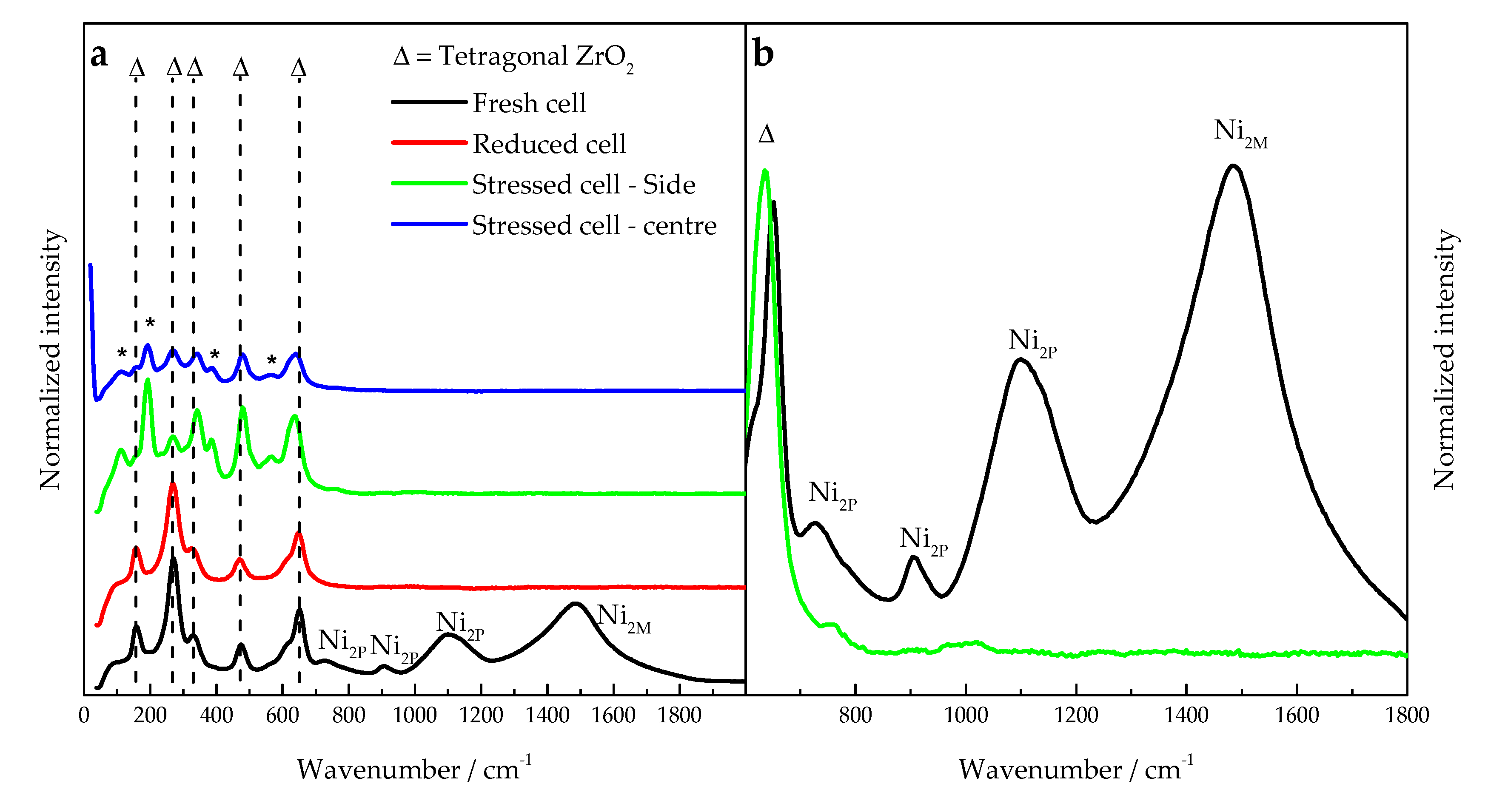
The diagnosis validation was achieved thanks to post-mortem analysis of the exhausted specimen. The exhausted SOC specimen was taken out from the testing apparatus for further characterizations, namely SEM analysis and Micro-Raman spectroscopy. In Figure 12, the SEMs of both fuel electrode face and section of the cell are shown. Looking at the cells section micrographs (A1 and B1), neither delamination’s were observed at the electrode-electrolyte interface nor cracks on the electrode. Concerning the micrographs of FE faces, no coarsening of both Ni catalyst and YSZ particles nor agglomeration were detected. This means that the high-current stress test did not irreversibly damage the cell. To have a clearer view of the microstructural composition of the FE, Micro-Raman spectroscopy was employed (Figure 13). The pristine cell presented all the characteristics peaks of YSZ and NiO. The peaks at 157 cm−1, 271 cm−1, 333 cm−1, 474 cm−1, and 650 cm−1 (labeled as Δ) can be assigned to tetragonal ZrO2 [48]. Four peaks assignable to NiO can be observed at a wavenumber higher than 700 cm−1. Specifically, the two-phonon 2nd order transverse optical mode at ≈ 730 cm−1 (Ni2P), the two-phonon mode transverse optical + longitudinal mode at ≈ 906 cm−1 (Ni2P), the two-phonon 2nd order longitudinal optical mode at ≈ 1090 cm−1 (Ni2P), and at last the two-magnon mode at ≈ 1500 cm−1 (2M) [49,50]. No peaks of the one-phonon mode (<700 cm−1) appear, probably because they overlapped with the scattering of YSZ. As the cell is started, the NiO in the FE is reduced with 100 % H2 at 150 Sml/min. Indeed, all the peaks coming from NiO scattering are no more visible, suggesting a complete reduction of NiO to metal Ni.
To study the composition on the exhausted SOC specimen, Raman spectra were acquired on two different spots, i.e., the center and near the circumference of the electrode. The peaks due to the scattering of tetragonal ZrO2 were still visible. Two peaks, which were at 474 cm−1 and 650 cm−1, shifted at 478 cm−1 and 640 cm−1, respectively. A new set of peaks appeared from 190 cm−1 up to 730 cm−1. These peaks were assigned to NiO as zone-boundary phonon mode (190 cm−1), one-phonon transverse optical mode (380 cm−1), one-phonon longitudinal optical mode (570 cm−1), and two-phonon 2nd order transverse optical mode (730 cm−1). The higher intensity of the one-phonon mode peaks can be explained by the defect-rich surface of the catalyst particles, probably induced by the stress test [49]. The two-phonon modes of NiO (>730 cm−1) could be weak because of two factors: (i) the surface layer is amorphous, and (ii) the presence of adsorbate species on the surface such as oxygen or water [50]. Finally, the absence of the two-magnon peak (1500 cm−1) could be due to the laser-induced heating above the Néel temperature and the destruction of magnetic ordering [51].
4. Discussion and Concluding Remarks
In the test here proposed, the stress agent causing early degradation of the SOC material was known a priori. Thus, the comprehensive analysis of the evolution of DRT peaks features (center and area) revealed the effect of the stress test. Similar experiences might be conducted, perturbating the SOC operation with different stress agents. Nonetheless, the experimental evidence, profusely presented and discussed in Section 3, already provides a validation of the diagnostic technique here proposed, encompassing EIS signal analysis and post-mortem SOC material investigation. Therefore, the technique based on EIS and DRT can be implemented as a tool for SOC operando diagnosis. Real-time deconvolution of EIS data and the comparison of results with new&clean deconvoluted spectra allow identifying faults outbreak and deliver specific information on the leading cause behind performance loss. The detection of faults at the early stage is fundamental for process control and management and permits mitigation actions to reduce the stress on the SOC material; hence, preventing its performance from decaying beyond physiological rates.
The diagnostic tool here presented is related to a particular family of hydrogen electrochemical energy technologies, namely Solid Oxide Cells. As presented in the Introduction, this technology embeds a great potential in both fuel cell and electrolysis processes, as well as in reversible operated cells. Moreover, the methodology adopted in the diagnostic tool shows relevance in the broader framework of hydrogen energy conversion technologies. Hence, provided that DRT peaks are correctly identified, their utilization can be extended beyond solid oxide cells.
Author Contributions
Conceptualization, L.B.; methodology, A.B.; software, A.S.; validation, A.B., and A.S.; formal analysis, A.S. and F.N.; investigation, A.B.; resources, L.B.; data curation, A.S.; writing—original draft preparation, A.B. and A.S.; writing—review and editing, L.B. and F.N.; visualization, A.B. and A.S.; supervision, G.B.; project administration, L.B.; funding acquisition, L.B. All authors have read and agreed to the published version of the manuscript.
Funding
This research was funded by the Italian Ministry for Education and Research (MIUR), under the program “Progetti di Ricerca di rilevante Interesse Nazionale” (PRIN-2017)” in the context of HERMES (High Efficiency Reversible technologies in fully renewable Multi-Energy System project)—Prot. 2017F4S2L3.
Institutional Review Board Statement
Not applicable.
Informed Consent Statement
Not applicable.
Data Availability Statement
Data sharing not applicable.
Conflicts of Interest
The authors declare no conflict of interest. The funders had no role in the design of the study; in the collection, analyses, or interpretation of data; in the writing of the manuscript, or in the decision to publish the results.
Abbreviations
| AE | Air Electrode |
| DAQ | Digital Acquistition System |
| DC | Direct Current |
| DRT | Distribution of Relaxation Times |
| ECM | Equivalent Circuit Model |
| EIS | Electrochemical Impedance Spectroscopy |
| FMC | Flow Meter Controller |
| FE | Fuel Electrode |
| HOR | Hydrogen Oxidation Reaction |
| MIEC | Mixed Ionic-Electronic Conductor |
| NLLS | Non-Linear Least Square |
| OC | Open Circuit |
| OCV | Open Circuit Voltage |
| ORR | Oxygen Reduction Reaction |
| rSOC | Reversible Solid Oxide Cell |
| RT | Room Temperature |
| SEM | Scanning Electron Microscopy |
| SOC | Solid Oxide Cell |
| SOFC | Solid Oxide Fuel Cell |
| TM | Temperature Measurement |
| TR | Temperature Regulation |
| YSZ | Yttria-stabilized Zirconia |
References
- Venkataraman, V.; Pérez-Fortes, M.; Wang, L.; Hajimolana, Y.S.; Boigues-Muñoz, C.; Agostini, A.; McPhail, S.J.; Maréchal, F.; Van Herle, J.; Aravind, P. Reversible solid oxide systems for energy and chemical applications—Review & perspectives. J. Energy Storage 2019, 24, 100782. [Google Scholar] [CrossRef] [Green Version]
- Posdziech, O.; Schwarze, K.; Brabandt, J. Efficient hydrogen production for industry and electricity storage via high-temperature electrolysis. Int. J. Hydrogen Energy 2019, 44, 19089–19101. [Google Scholar] [CrossRef]
- Bicer, Y.; Khalid, F. Life cycle environmental impact comparison of solid oxide fuel cells fueled by natural gas, hydrogen, ammonia and methanol for combined heat and power generation. Int. J. Hydrogen Energy 2020, 45, 3670–3685. [Google Scholar] [CrossRef]
- Choudhury, A.; Chandra, H.; Arora, A. Application of solid oxide fuel cell technology for power generation—A review. Renew. Sustain. Energy Rev. 2013, 20, 430–442. [Google Scholar] [CrossRef]
- Keçebaş, A.; Kayfeci, M.; Bayat, M. Electrochemical hydrogen generation. In Solar Hydrogen Production; Elsevier: Amsterdam, The Netherlands, 2019; pp. 299–317. [Google Scholar]
- David, M.; Ocampo-Martínez, C.; Sánchez-Peña, R. Advances in alkaline water electrolyzers: A review. J. Energy Storage 2019, 23, 392–403. [Google Scholar] [CrossRef] [Green Version]
- Bianchi, F.R.; Baldinelli, A.; Barelli, L.; Cinti, G.; Audasso, E.; Bosio, B. Multiscale Modeling for Reversible Solid Oxide Cell Operation. Energies 2020, 13, 5058. [Google Scholar] [CrossRef]
- Frank, M.; Deja, R.; Peters, R.; Blum, L.; Stolten, D. Bypassing renewable variability with a reversible solid oxide cell plant. Appl. Energy 2018, 217, 101–112. [Google Scholar] [CrossRef]
- Nguyen, V.N.; Fang, Q.; Packbier, U.; Blum, L. Long-term tests of a Jülich planar short stack with reversible solid oxide cells in both fuel cell and electrolysis modes. Int. J. Hydrogen Energy 2013, 38, 4281–4290. [Google Scholar] [CrossRef]
- Hanasaki, M.; Uryu, C.; Daio, T.; Kawabata, T.; Tachikawa, Y.; Lyth, S.M.; Shiratori, Y.; Taniguchi, S.I.; Sasaki, K. SOFC Durability against Standby and Shutdown Cycling. J. Electrochem. Soc. 2014, 161, F850–F860. [Google Scholar] [CrossRef]
- Cooper, S.J.; Brandon, N.P. An Introduction to Solid Oxide Fuel Cell Materials, Technology and Applications; Elsevier Ltd.: Amsterdam, The Netherlands, 2017. [Google Scholar]
- Petipas, F.; Fu, Q.; Brisse, A.; Bouallou, C. Transient operation of a solid oxide electrolysis cell. Int. J. Hydrogen Energy 2013, 38, 2957–2964. [Google Scholar] [CrossRef]
- Preininger, M.; Stoeckl, B.; Subotić, V.; Hochenauer, C.; Stöckl, B. Extensive analysis of an SOC stack for mobile application in reversible mode under various operating conditions. Electrochimica Acta 2019, 299, 692–707. [Google Scholar] [CrossRef]
- Baldinelli, A.; Barelli, L.; Bidini, G.; Discepoli, G. Economics of innovative high capacity-to-power energy storage technologies pointing at 100% renewable micro-grids. J. Energy Storage 2020, 28, 101198. [Google Scholar] [CrossRef]
- Pfeifer, T.; Reuber, S.; Hartmann, M.; Barthel, M.; Baade, J.; Matyáš, J.; Balaya, P.; Singh, D.; Wei, J. SOFC System Development and Held Trials for Commercial Applications. Process. High Temp. Supercond. 2016, 255, 61–75. [Google Scholar] [CrossRef]
- Khan, M.S.; Lee, S.-B.; Song, R.-H.; Lee, J.-W.; Lim, T.-H.; Park, S.-J. Fundamental mechanisms involved in the degradation of nickel–yttria stabilized zirconia (Ni–YSZ) anode during solid oxide fuel cells operation: A review. Ceram. Int. 2016, 42, 35–48. [Google Scholar] [CrossRef]
- Sasaki, K.; Susuki, K.; Iyoshi, A.; Uchimura, M.; Imamura, N.; Kusaba, H.; Teraoka, Y.; Fuchino, H.; Tsujimoto, K.; Uchida, Y.; et al. H2S Poisoning of Solid Oxide Fuel Cells. J. Electrochem. Soc. 2006, 153, A2023–A2029. [Google Scholar] [CrossRef]
- Sreedhar, I.; Agarwal, B.; Goyal, P.; Agarwal, A. An overview of degradation in solid oxide fuel cells-potential clean power sources. J. Solid State Electrochem. 2020, 24, 1239–1270. [Google Scholar] [CrossRef]
- Jiang, S.P.; Zhen, Y. Mechanism of Cr deposition and its application in the development of Cr-tolerant cathodes of solid oxide fuel cells. Solid State Ionics 2008, 179, 1459–1464. [Google Scholar] [CrossRef]
- Fergus, J. Effect of cathode and electrolyte transport properties on chromium poisoning in solid oxide fuel cells. Int. J. Hydrogen Energy 2007, 32, 3664–3671. [Google Scholar] [CrossRef]
- Trembly, J.; Gemmen, R.; Bayless, D. The effect of coal syngas containing HCl on the performance of solid oxide fuel cells: Investigations into the effect of operational temperature and HCl concentration. J. Power Sources 2007, 169, 347–354. [Google Scholar] [CrossRef]
- El Gabaly, F.; Mccarty, K.F.; Bluhm, H.; McDaniel, A.H. Oxidation stages of Ni electrodes in solid oxide fuel cell environments. Phys. Chem. Chem. Phys. 2013, 15, 8334–8341. [Google Scholar] [CrossRef]
- Li, X.; Blinn, K.; Chen, D.; Liu, M. In Situ and Surface-Enhanced Raman Spectroscopy Study of Electrode Materials in Solid Oxide Fuel Cells. Electrochem. Energy Rev. 2018, 1, 433–459. [Google Scholar] [CrossRef]
- Li, X.; Lee, J.-P.; Blinn, K.S.; Chen, D.; Yoo, S.; Kang, B.; Bottomley, L.A.; El-Sayed, M.A.; Park, S.; Liu, M. High-temperature surface enhanced Raman spectroscopy for in situ study of solid oxide fuel cell materials. Energy Environ. Sci. 2013, 7, 306–310. [Google Scholar] [CrossRef] [Green Version]
- Swallow, J.G.; Lee, J.K.; Defferriere, T.; Hughes, G.M.; Raja, S.N.; Tuller, H.L.; Warner, J.H.; Van Vliet, K.J. Atomic Resolution Imaging of Nanoscale Chemical Expansion in PrxCe1−xO2−δ during In Situ Heating. ACS Nano 2018, 12, 1359–1372. [Google Scholar] [CrossRef]
- Hwang, S.; Chen, X.; Zhou, G.; Su, D. In Situ Transmission Electron Microscopy on Energy-Related Catalysis. Adv. Energy Mater. 2020, 10, 1902105. [Google Scholar] [CrossRef]
- Stangl, A.; Munoz-Rojas, D.; Burriel, M. In situ and operando characterisation techniques for solid oxide electrochemical cells: Recent advances. J. Phys. Energy 2020, 3, 12001. [Google Scholar] [CrossRef]
- Baldinelli, A.; Barelli, L.; Bidini, G.; Di Cicco, A.; Gunnella, R.; Minicucci, M.; Trapananti, A. Advancements regarding in-operando diagnosis techniques for solid oxide cells NiYSZ cermets. AIP Conf. Proc. 2019, 2191, 020012. [Google Scholar] [CrossRef]
- Nielsen, J.; Hjelm, J. Impedance of SOFC electrodes: A review and a comprehensive case study on the impedance of LSM:YSZ cathodes. Electrochimica Acta 2014, 115, 31–45. [Google Scholar] [CrossRef] [Green Version]
- Nobili, F.; Tossici, R.; Marassi, R.; Croce, F.; Scrosati, B. An AC Impedance Spectroscopic Study of LixCoO2 at Different Temperatures. J. Phys. Chem. B 2002, 106, 3909–3915. [Google Scholar] [CrossRef]
- Pitarch-Tena, D.; Ngo, T.T.; Vallés-Pelarda, M.; Pauporté, T.; Mora-Seró, I. Impedance Spectroscopy Measurements in Perovskite Solar Cells: Device Stability and Noise Reduction. ACS Energy Lett. 2018, 3, 1044–1048. [Google Scholar] [CrossRef] [Green Version]
- Schwartz, M. The theory of impedance in biological systems. J. Biol. Phys. 1973, 1, 123–142. [Google Scholar] [CrossRef]
- Kornely, M.; Neumann, A.; Menzler, N.H.; Leonide, A.; Weber, A.; Ivers-Tiffée, E. Degradation of anode supported cell (ASC) performance by Cr-poisoning. J. Power Sources 2011, 196, 7203–7208. [Google Scholar] [CrossRef]
- Kromp, A.; Dierickx, S.; Leonide, A.; Weber, A.; Iverstiffee, E. Electrochemical Analysis of Sulfur-Poisoning in Anode Supported SOFCs Fuelled with a Model Reformate. J. Electrochem. Soc. 2012, 159, B597–B601. [Google Scholar] [CrossRef]
- Sumi, H.; Shimada, H.; Yamaguchi, Y.; Yamaguchi, T.; Fujishiro, Y. Degradation evaluation by distribution of relaxation times analysis for microtubular solid oxide fuel cells. Electrochimica Acta 2020, 339, 135913. [Google Scholar] [CrossRef]
- Dierickx, S.; Weber, A.; Ivers-Tiffée, E. How the distribution of relaxation times enhances complex equivalent circuit models for fuel cells. Electrochimica Acta 2020, 355, 136764. [Google Scholar] [CrossRef]
- Boukamp, B.A. A Nonlinear Least Squares Fit procedure for analysis of immittance data of electrochemical systems. Solid State Ionics 1986, 20, 31–44. [Google Scholar] [CrossRef] [Green Version]
- Macdonald, J.R. Impedance spectroscopy: Old problems and new developments. Electrochimica Acta 1990, 35, 1483–1492. [Google Scholar] [CrossRef]
- Bartoszek, J.; Liu, Y.-X.; Karczewski, J.; Wang, S.-F.; Mrozinski, A.; Jasiński, P. Distribution of relaxation times as a method of separation and identification of complex processes measured by impedance spectroscopy. In Proceedings of the 2017 21st European Microelectronics and Packaging Conference (EMPC) & Exhibition, Warsaw, Poland, 10–13 September 2017; pp. 1–5. [Google Scholar]
- Baldinelli, A.; Staffolani, A.; Bidini, G.; Barelli, L.; Nobili, F. An extensive model for renewable energy electrochemical storage with Solid Oxide Cells based on a comprehensive analysis of impedance deconvolution. J. Energy Storage 2021, 33, 102052. [Google Scholar] [CrossRef]
- Boukamp, B. Practical application of the Kramers-Kronig transformation on impedance measurements in solid state electrochemistry. Solid State Ionics 1993, 62, 131–141. [Google Scholar] [CrossRef] [Green Version]
- Wan, T.H.; Saccoccio, M.; Chen, C.; Ciucci, F. Influence of the Discretization Methods on the Distribution of Relaxation Times Deconvolution: Implementing Radial Basis Functions with DRTtools. Electrochimica Acta 2015, 184, 483–499. [Google Scholar] [CrossRef]
- Papurello, D.; Menichini, D.; Lanzini, A. Distributed relaxation times technique for the determination of fuel cell losses with an equivalent circuit model to identify physicochemical processes. Electrochimica Acta 2017, 258, 98–109. [Google Scholar] [CrossRef]
- Muñoz, C.B.; Pumiglia, D.; McPhail, S.J.; Montinaro, D.; Comodi, G.; Santori, G.; Carlini, M.; Polonara, F. More accurate macro-models of solid oxide fuel cells through electrochemical and microstructural parameter estimation—Part I: Experimentation. J. Power Sources 2015, 294, 658–668. [Google Scholar] [CrossRef] [Green Version]
- Leonide, A.; Sonn, V.; Weber, A.; Ivers-Tiffée, E. Evaluation and Modeling of the Cell Resistance in Anode-Supported Solid Oxide Fuel Cells. J. Electrochem. Soc. 2008, 155, B36–B41. [Google Scholar] [CrossRef]
- Macdonald, J.R. Impedance Spectroscopy: Emphasizing Solid Materials and Systems; Wiley-Interscience: Hoboken, NJ, USA, 1987. [Google Scholar]
- Adler, S.B.; Lane, J.A.; Steele, B.C.H. Electrode Kinetics of Porous Mixed-Conducting Oxygen Electrodes. J. Electrochem. Soc. 1996, 143, 3554–3564. [Google Scholar] [CrossRef]
- Basahel, S.N.; Ali, T.T.; Mokhtar, M.; Narasimharao, K. Influence of crystal structure of nanosized ZrO2 on photocatalytic degradation of methyl orange. Nanoscale Res. Lett. 2015, 10, 73. [Google Scholar] [CrossRef] [Green Version]
- Mironova-Ulmane, N.; Kuzmin, A.; Steins, I.; Grabis, J.; Sildos, I.; Pärs, M. Raman scattering in nanosized nickel oxide NiO. J. Phys. Conf. Ser. 2007, 93, 012039. [Google Scholar] [CrossRef]
- Burmistrov, I.; Agarkov, D.; Tartakovskii, I.; Kharton, V.; Bredikhin, S. Performance Optimization of Cermet SOFC Anodes: An Evaluation of Nanostructured NiO. ECS Meet. Abstr. 2015, 68, 1265–1274. [Google Scholar] [CrossRef] [Green Version]
- Mironova-Ulmane, N.; Kuzmin, A.; Sildos, I.; Puust, L.; Grabis, J. Magnon and Phonon Excitations in Nanosized NiO. Latv. J. Phys. Tech. Sci. 2019, 56, 61–72. [Google Scholar] [CrossRef] [Green Version]
Figure 1.
Typical EIS spectrum for a SOC (a), and its DRT deconvolution (b).

Figure 2.
Equivalent circuit model for the SOC type used in this experiment. The model is tuned on a cell with a NiYSZ fuel electrode and GDC/LSCF air electrode.
Figure 2.
Equivalent circuit model for the SOC type used in this experiment. The model is tuned on a cell with a NiYSZ fuel electrode and GDC/LSCF air electrode.
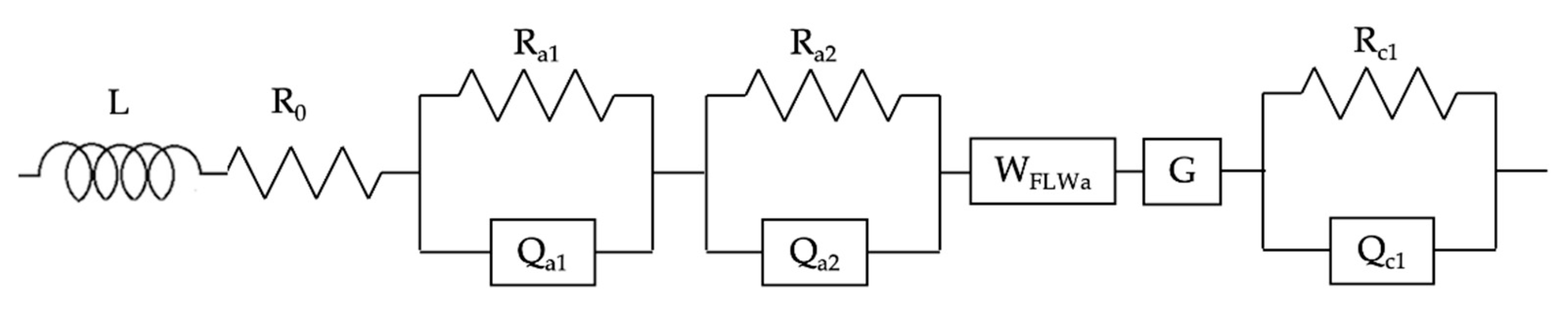
Figure 3.
Conceptual workflow chart.
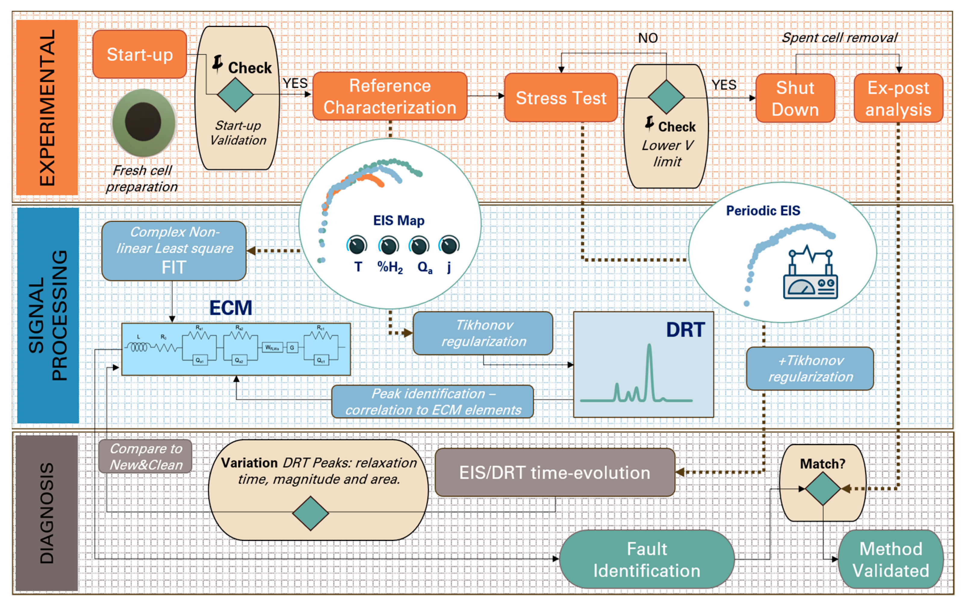
Figure 4.
Testing apparatus schematic (cell, housing, and measurement hardware).

Figure 5.
Polarization characterization: Begin reference versus endpoint i-V curve.
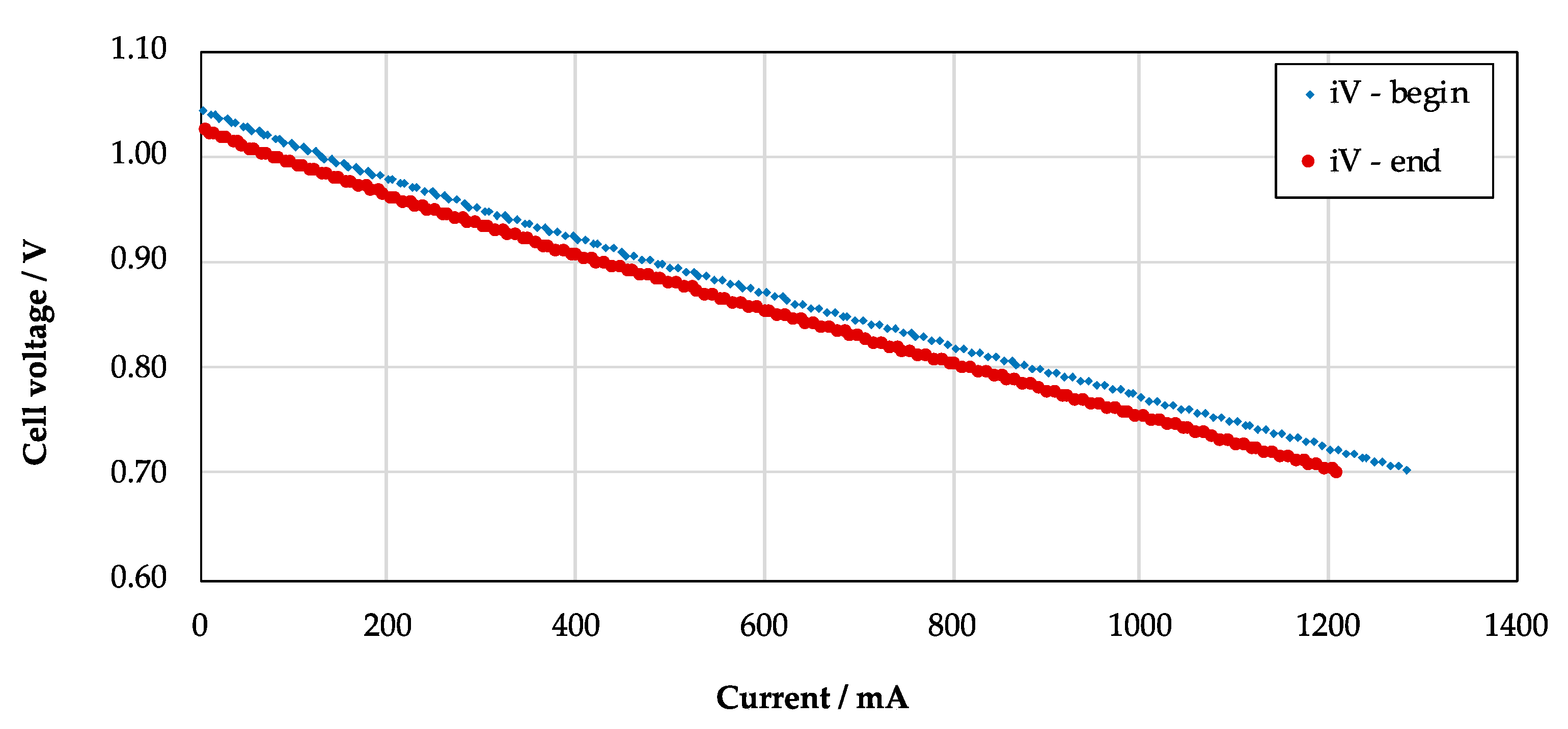
Figure 6.
Test history through voltage and current data logs. Monitoring spots are flagged.

Figure 7.
(a) Experimental (blue empty scatter) and Fitted (solid red line) impedance spectrum acquired at 1048 K with H2:N2 25:75 200 Sml/min at the anode and air at 300 Sml/min at the AE, (b) DRT of the impedance spectrum with the assigned peaks, (c) Kramer-Kronig residuals of the real part of the impedance spectrum, (d) residuals of the real part of impedance spectrum after fitting with the proposed ECM.
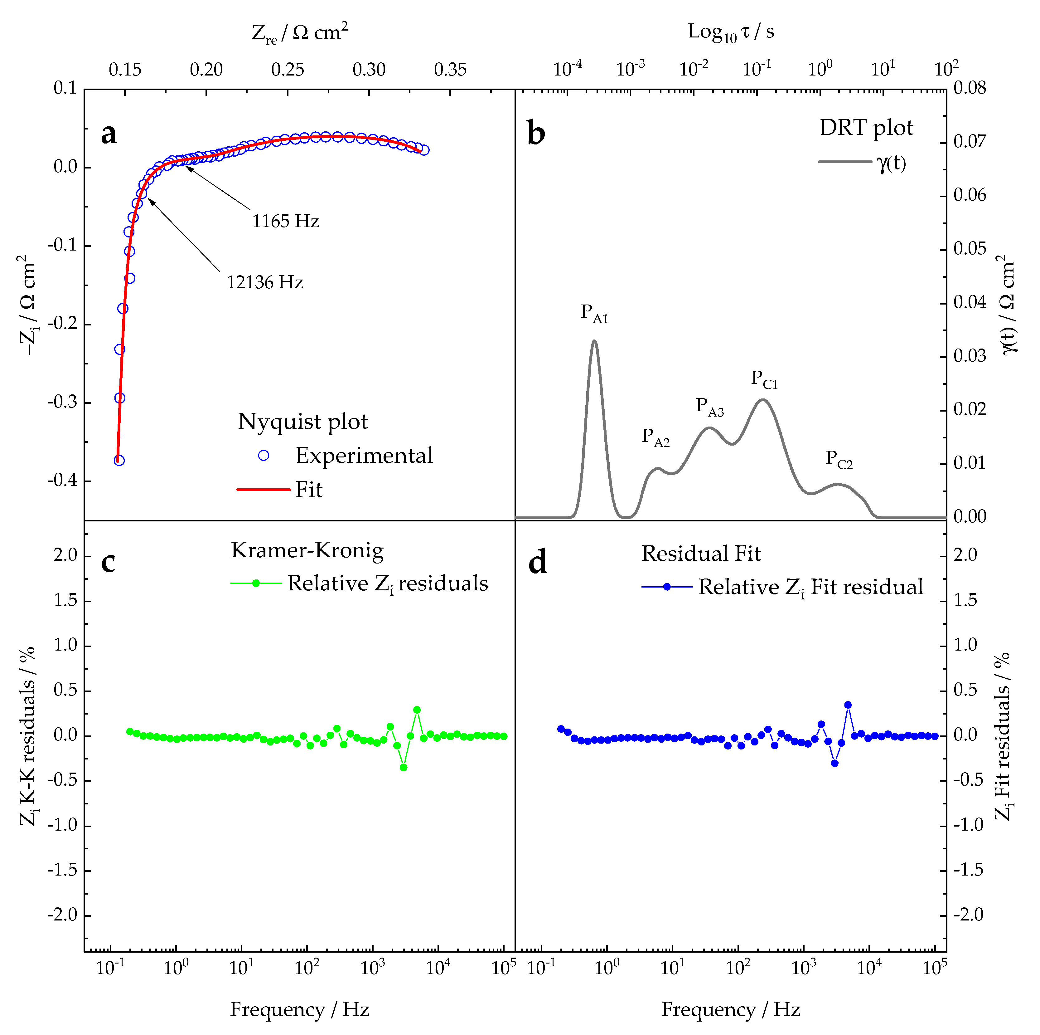
Figure 8.
Nyquist plots acquired at begin ref (a), after 28 h (b), and at the endpoint of the experiment (c) at three different current densities, i.e., 0, 250, and 500 mA/cm2; DRT plot of the above-mentioned impedance spectrum: begin ref (d), after 28 h (e), and at the endpoint of experiment (f).
Figure 8.
Nyquist plots acquired at begin ref (a), after 28 h (b), and at the endpoint of the experiment (c) at three different current densities, i.e., 0, 250, and 500 mA/cm2; DRT plot of the above-mentioned impedance spectrum: begin ref (d), after 28 h (e), and at the endpoint of experiment (f).

Figure 9.
Fitted DRT plot by the Gaussian function. The shape of the peaks is highlighted.
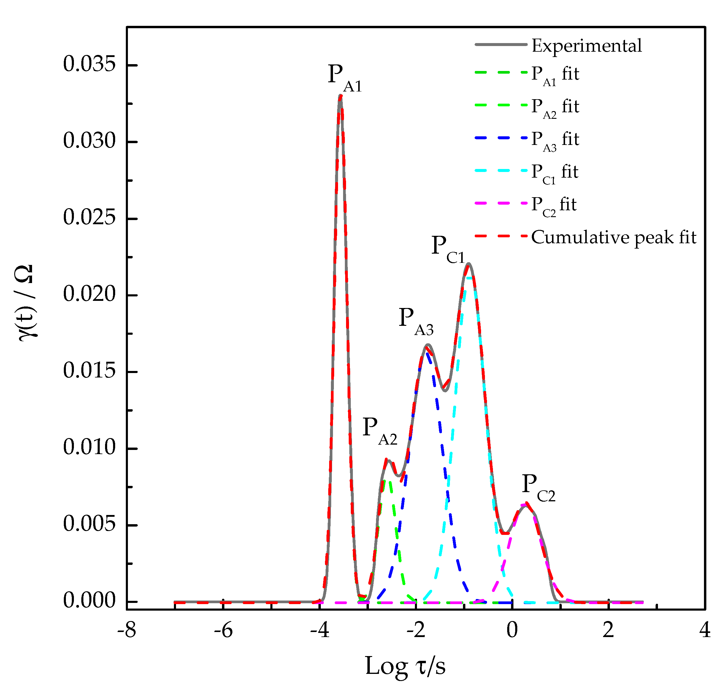
Figure 10.
Relaxation time and area as a function of the experiment time. T = 1048 K, H2:N2 27:75 200 Sml/min at the FE, air 300 Sml/min at the AE, j = 250 mA/cm2.
Figure 10.
Relaxation time and area as a function of the experiment time. T = 1048 K, H2:N2 27:75 200 Sml/min at the FE, air 300 Sml/min at the AE, j = 250 mA/cm2.

Figure 11.
Relaxation time and area as a function of the experiment time. T = 1048 K, H2:N2 27:75 200 Sml/min at the FE, air 300 Sml/min at the AE, j = 500 mA/cm2.
Figure 11.
Relaxation time and area as a function of the experiment time. T = 1048 K, H2:N2 27:75 200 Sml/min at the FE, air 300 Sml/min at the AE, j = 500 mA/cm2.
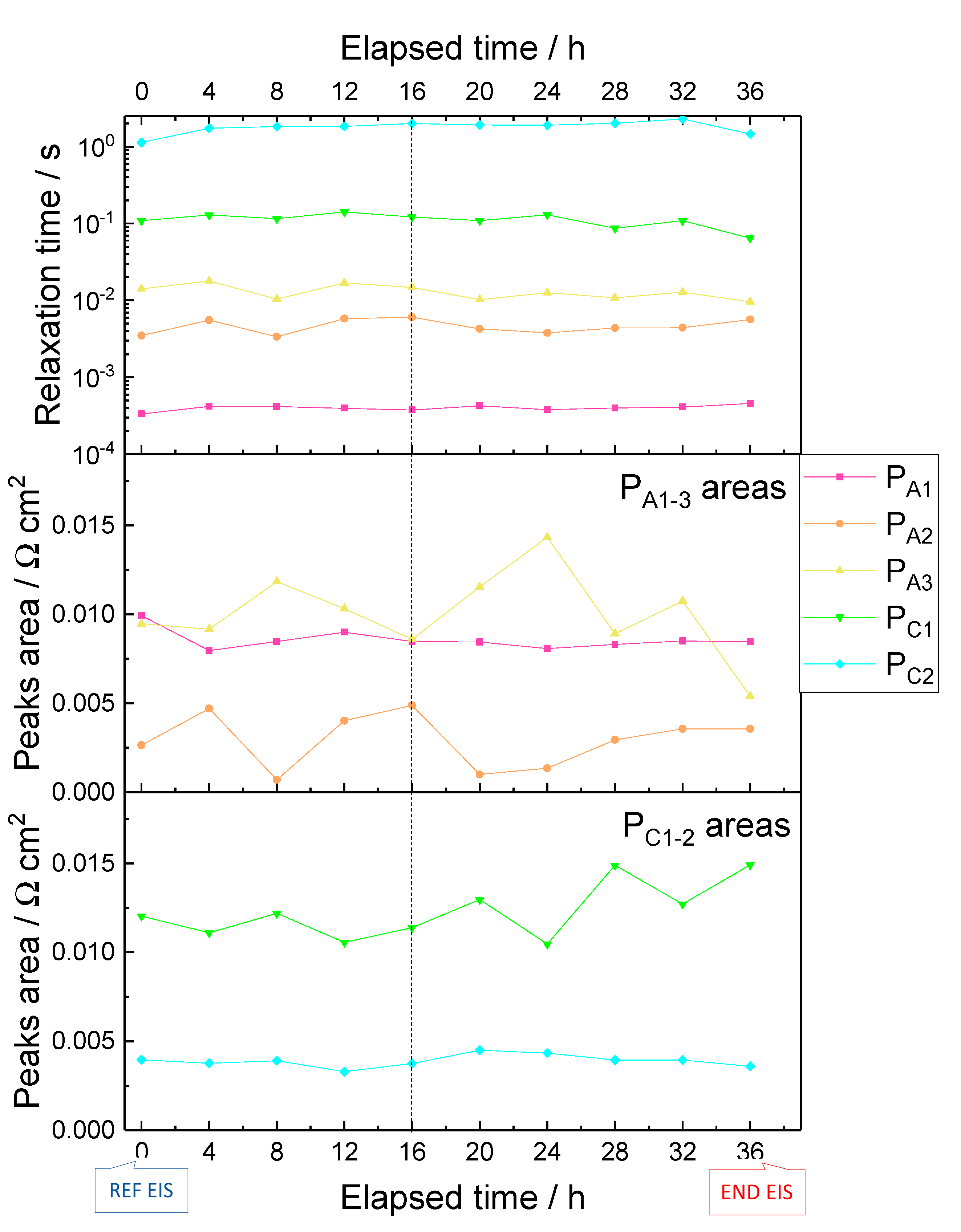
Figure 12.
SEM micrographs of both section (800 × magnification) and anode face (20 kx magnification) of the pristine cell after reduction (A1,A2) and stressed SOC specimen (B1,B2).
Figure 12.
SEM micrographs of both section (800 × magnification) and anode face (20 kx magnification) of the pristine cell after reduction (A1,A2) and stressed SOC specimen (B1,B2).

Figure 13.
(a) Raman spectra of the pristine cell (black line), pristine reduced cell (red line), side of exhausted SOC specimen (green line), the center of exhausted SOC specimen (blue line). (b) Comparison of pristine cell and exhausted SOC specimen from 600 up to 1800 cm−1.
Figure 13.
(a) Raman spectra of the pristine cell (black line), pristine reduced cell (red line), side of exhausted SOC specimen (green line), the center of exhausted SOC specimen (blue line). (b) Comparison of pristine cell and exhausted SOC specimen from 600 up to 1800 cm−1.

Table 1.
Physicochemical phenomena occurring in the SOC vs. ECM notation.
| Phenomenon | Variation With: | DRT Peak | ECM Element |
|---|---|---|---|
| Oxygen transport | Temperature | PA1 at τ = 10−4 s | Ra1Qa1 = |
| HOR | Hydrogen partial pressure, catalytic activity at the FE, temperature | PA2 at τ = 10−3 s | Ra2Qa2 = |
| ORR | Oxygen partial pressure, catalytic activity at the AE, temperature | PC1 at τ = 10−1 s | Rc1QC1 = |
| Mass transport FE (NiYSZ) | Reactants space velocity, utilization rate (current density) at the FE | PA3 at τ = 10−2 s | WFLWa = |
| Mass transport AE (GDC/LSCF) | Reactants space velocity, utilization rate (current density) at the AE | PC2 at τ = 10 s | G = |
| Electrolyte | Temperature | - | R0 |
| Wiring—Cell geometry | Not relevant | - |
Table 2.
Solid oxide cell features.
| Layer | Composition | Thickness |
|---|---|---|
| Fuel Electrode | NiYSZ | 240 μm |
| Electrolyte | 8YSZ | 8 μm |
| Air Electrode | GDC-LSCF | 50 μm |
Table 3.
Test protocol: electrode feeding gases flowrates and composition, and cell operating settings (Legend: X = volume composition [%vol dry basis], Q = volume flow rate [Sml/min], T = temperature [K]. The stress test is repeated until a noticeable performance decay is measured.
Table 3.
Test protocol: electrode feeding gases flowrates and composition, and cell operating settings (Legend: X = volume composition [%vol dry basis], Q = volume flow rate [Sml/min], T = temperature [K]. The stress test is repeated until a noticeable performance decay is measured.
| TEST | Fuel Electrode | Air Electrode | Operating Settings | Duration | |||
|---|---|---|---|---|---|---|---|
| ID | X | Q | x | Q | T | Load | Hours |
| Start-up | 100% N2 | 50 | 21% O2 + 79% N2 | 300 | RT1 → 1073 | OC | 16 h |
| Reduction | 100% N2 → 100% H2 | 150 | 21% O2 + 79% N2 | 300 | 1073 | OC | 1.5 h |
| Stabilization | 100% H2 | 150 | 21% O2 + 79% N2 | 300 | 1073 | Constant j = 250 mA/cm2 | 100 h |
| Begin Ref | 25% H2 + 75% N2 | 200 | 21% O2 + 79% N2 | 300 | 1048 | i-V: OC → 0.7 V EIS: 0, 100, 250, 500, 750 mA/cm2 | 30 min 1 h |
| Stress test (repeated) | 25% H2 + 75% N2 | 200 | 21% O2 + 79% N2 | 300 | 1048 | Constant j = 1500 mA/cm2 EIS: 0, 100, 250, 500 mA/cm2 | 4 h 30 min |
| End Point | 25% H2 + 75% N2 | 200 | 21% O2 + 79% N2 | 300 | 1048 | i-V: OC → 0.7 V EIS: 0, 100, 250, 500, 750 mA/cm2 | 30 min 1 h |
| Shut down | 5% H2 + 95% N2 | 100 | 100% N2 | 100 | 1073 → RT | OC | c.a. 12 h |
Publisher’s Note: MDPI stays neutral with regard to jurisdictional claims in published maps and institutional affiliations. |
© 2021 by the authors. Licensee MDPI, Basel, Switzerland. This article is an open access article distributed under the terms and conditions of the Creative Commons Attribution (CC BY) license (https://creativecommons.org/licenses/by/4.0/).
Share and Cite
MDPI and ACS Style
Staffolani, A.; Baldinelli, A.; Barelli, L.; Bidini, G.; Nobili, F. Early-Stage Detection of Solid Oxide Cells Anode Degradation by Operando Impedance Analysis. Processes 2021, 9, 848. https://doi.org/10.3390/pr9050848
AMA Style
Staffolani A, Baldinelli A, Barelli L, Bidini G, Nobili F. Early-Stage Detection of Solid Oxide Cells Anode Degradation by Operando Impedance Analysis. Processes. 2021; 9(5):848. https://doi.org/10.3390/pr9050848
Chicago/Turabian StyleStaffolani, Antunes, Arianna Baldinelli, Linda Barelli, Gianni Bidini, and Francesco Nobili. 2021. "Early-Stage Detection of Solid Oxide Cells Anode Degradation by Operando Impedance Analysis" Processes 9, no. 5: 848. https://doi.org/10.3390/pr9050848
Note that from the first issue of 2016, this journal uses article numbers instead of page numbers. See further details here.