
Identification of Granule Growth Regimes in High Shear Wet Granulation Processes Using a Physics-Constrained Neural Network

Department of Chemical and Biochemical Engineering, Rugters, The State University of New Jersey, Piscataway, NJ 08854, USA
*
Author to whom correspondence should be addressed.
Processes 2021, 9(5), 737; https://doi.org/10.3390/pr9050737
Submission received: 5 March 2021
/
Revised: 16 April 2021
/
Accepted: 16 April 2021
/
Published: 22 April 2021
Abstract
:The digitization of manufacturing processes has led to an increase in the availability of process data, which has enabled the use of data-driven models to predict the outcomes of these manufacturing processes. Data-driven models are instantaneous in simulate and can provide real-time predictions but lack any governing physics within their framework. When process data deviates from original conditions, the predictions from these models may not agree with physical boundaries. In such cases, the use of first-principle-based models to predict process outcomes have proven to be effective but computationally inefficient and cannot be solved in real time. Thus, there remains a need to develop efficient data-driven models with a physical understanding about the process. In this work, we have demonstrate the addition of physics-based boundary conditions constraints to a neural network to improve its predictability for granule density and granule size distribution (GSD) for a high shear granulation process. The physics-constrained neural network (PCNN) was better at predicting granule growth regimes when compared to other neural networks with no physical constraints. When input data that violated physics-based boundaries was provided, the PCNN identified these points more accurately compared to other non-physics constrained neural networks, with an error of <1%. A sensitivity analysis of the PCNN to the input variables was also performed to understand individual effects on the final outputs.
1. Introduction
The manufacturing industry’s adoption of digitization has led to rapid growth in the available data [1]. This in turn has led to a foray of data-driven methods being used to predict the process operations [2]. These methods have successfully recognized patterns and have provided other useful insights in data-rich fields such as image and speech recognition. Machine learning techniques applied to manufacturing can automate several time-consuming tasks of knowledge acquisition [3]. The chemical industry has already incorporated artifical intelligence (AI) in process operations and diagnosis. General Electric and British Petroleum have used deep learning to monitor deep sea oil-well performance as well as reduce downtime [4]. Unlike big oil companies, the scale of data collection in other chemical industries is considerably smaller and may not provide sufficient data for machine learning methods to perform efficiently.
Chemical processes are governed by fundamental laws and laws of physics, which have led to the development of several high-fidelity models to predict process operations fairly accurately [5]. These models are inherently slower to simulate. These first-principle models when combined with high-throughput experiments have the ability to produce large amounts of data that can be used to train data-driven models [2]. Data-driven approaches have been able to predict processes with complex physical phenomena accurately, when trained using large amounts of data [6]. One such chemical industry where data-driven models can be useful is the formulated products industry, where the modeling of chaotic particulate flow is challenging.
Formulated particulate products are often used in the food, pharmaceutical, agriculture, and specialty chemical industries contribute to about half of the world’s chemical production [7]. Frequently, these formulated products are multi-component and their critical quality attributes (CQAs) are dependent on their product structure as well as the chemical composition [8]. With the increasing demand for performance criteria of formulated products, product manufacturing is becoming more complex in nature [9]. Granulation is an example of a particulate process that is of interest to the pharmaceutical industry. Granulation processes are complex and non-linear in nature making it difficult to capture all the physical phenomena inside a physics-based model [10] and data-driven models have not been successful in leveraging the underlying physical laws to extract patterns from the data. This deviation of predictions of the process model from the actual process can lead to a lot of risk during the manufacturing process. According to the US-FDA guidelines, the assessment of risk is important during the filing of the manufacturing process [11]. Risk assessment can aid in identifying the effects of material attributes and process parameters potentially have on the product CQAs. This assessment needs to be performed throughout the process development process. However, with current physics-based models being used for granulation, the qulaity assessment may not always be accurate. Thus, there is a need to integrate both the laws of physics as well as data-driven models for a more accurate prediction of quality attributes and identify the effects of each input parameter on them. This assessment can further be used to identify process characteristics which can predict failures of granulation batches before further processing, thus reducing manufacturing costs.
Some chemical process models have successfully integrated first-principle models with data-driven methods to create hybrid models and have shown promise in predicting process outcomes efficiently [12,13,14]. The data-driven component of these techniques only reduces the error between the first-principle model and the experimental data by adding a correction factor and its performance is dependent on the output from the first principle model. The data-driven model fails to incorporate any physical patterns that may be present in the process within itself. Introducing physics laws and constraints to data-driven models have proven to be very effective in incorporating some physics within the models themselves and have the ability to accuratley predict process outcomes [6,15,16,17].
Objectives
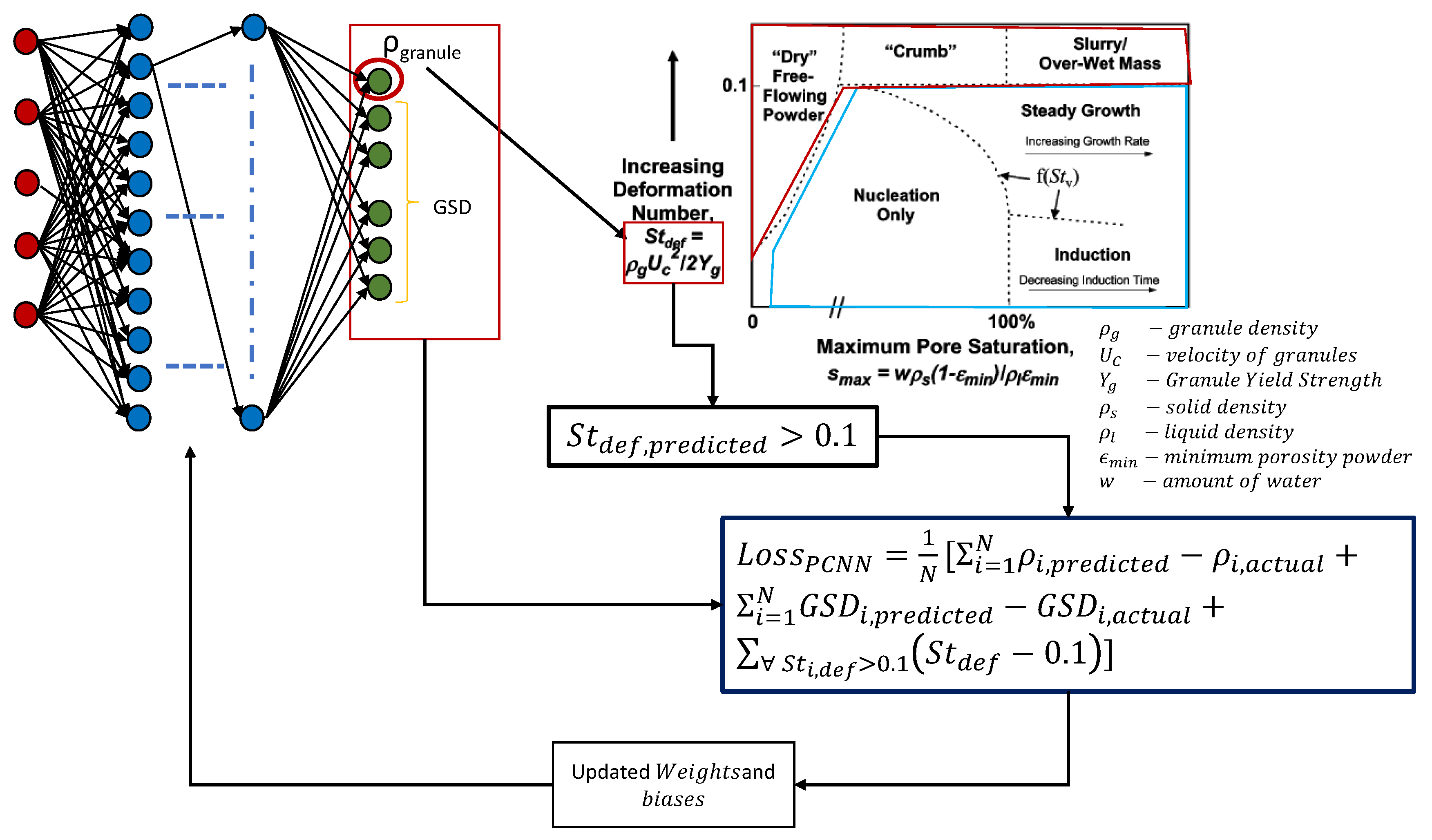
In this work, we propose a data-driven modeling framework that enables the incorporation of granulation rate governing laws from regime maps combined with the efficiency and accuracy of neural networks. In this physics-constrained neural network (PCNN) algorithm, the Stokes deformation () number was used to constraint the output of the neural network. This constraint meant that the PCNN added an extra regularization term onto the neural network, making the neural network more sensitive to predictions which lie in the crumb or slurry region of the regime map. The data used to develop these models is obtained by simulating an experimentally verified population balance model. The results from the PCNN are also compared to an ANN with no physics constraints and to an ANN trained with filtered steady state growth data. A sensitivity analysis of the inputs on the final GSD and granule density was also performed for better risk assessment.
2. Background
2.1. Wet Granulation and Population Balance Model
Wet granulation is a process of agglomeration of smaller particles into larger granules to improve flowability and compressibility. It is considered as an important unit operation in the solid processing industry [18]. In the pharmaceutical industry, wet granulation is employed during the downstream processing of solid dosage forms such as tablets from powder blends consisting of active pharmaceutical ingredients (APIs) and excipients. Wet granulation often involves the spraying of a liquid binder onto an agitated powder mixture [19]. The particles are bound together by a combination of capillary and viscous forces. This process is of economic importance to the pharmaceutical industry as it improves several characteristics of a tablet such as dissolution, hardness, etc. One of the earliest attempts to model the granulation process proposed by [20], where the researchers employed the use of population balance equations.
Ramakrishna et al. [21] have defined the population balance model (PBM) as a system of partial differential equations of a number conservation of entities inside a system. PBMs are able to describe various underlying granulation mechanisms that lead to the size enlargement of primary powder blends. PBMs can track several particle traits such as size, velocity, position, and the number of particle traits tracked are also referred to as the dimensions of the PBM [22].
Population balance models have been widely used to model the wet granulation process [23,24,25,26]. Since the PBM solution involves solving a system of ordinary differential equations at every timestep, they are inherently slow to simulate. There have been attempts made to solve these PBMs faster by exploiting CPU-based parallel computing [27,28,29], graphic processing units (GPUs) [30,31], as well as using high performance computing tools or supercomputers [29,32]. These models were only able to reduce the time of simulation down to minutes. Thus, there is still a need for models that can generate predictions in real-time for process control.
2.2. Artificial Neural Networks
Artificial neural networks (ANN) are very efficient function approximators as they create a non-linear relationship between the inputs and outputs, with the help of weights and biases. This is achieved with the help of simple elements called neurons or nodes. Each neuron can make simple decisions and pass these decisions onto other neurons [33]. A typical neural network comprises of an input layer, a hidden layer(s), and an output layer. The number of nodes in each layer varies according to the use. The number of nodes in the input layer usually correspond to the input data dimensions and the same is true for the output layer of the ANN as well. The number of hidden layers and the number of nodes inside the ANN can vary with the application and the most optimal combination is obtained by trial and error. Some studies have developed recursive algorithms [34] though such methods are iterative and slow.
Each neuron within each layer can have multiple inputs as well as outputs. The output of one neuron of a hidden layer serves as the input to neurons in the next layer. The output of a neuron is determined by a combination of weights, biases, and the activation function chosen. The mathematical representation of a neuron is given by Equations (1) and (2):
where, i is a neuron number in the layer l, is the corresponding weight for each input to the neuron, and is the bias for the neuron, which helps build linear models that are not fixed at the origin. represents the output of the neuron i in layer l after activation. Similarly, the activations of all neurons for a given layer l can be calculated by Equation (3).
where and are the matrix forms of the outputs and weights, respectively.
This process of forward-propagation of outputs culminates at the output layer of the neural network and the error is calculated against the provided data. The error is then used to update the weights and biases for each neuron using the gradient [35]. This process is also called back-propagation. A combination of one forward-propagating error calculation and one back-propagating hyperparameter update is known as one epoch. Several such epochs are required to help train the neural network effectively.
The performance of a neural network is dependent on the data presented to it during training. However, data are not the only factors that can affect its ability to predict. Several modifications can be made to the neural network algorithm for it to predict data accurately. One important algorithmic change could be changing the optimization technique used. This would then affect how the parameters are updated. The number of epochs is also a hyperparameter that could affect the accuracy of the ANN, but a very high epoch number could also lead to an over-fitted network. Over-fitting can be addressed in neural networks either by adding activity regularization to the outputs or by using dropout. Dropout refers to hiding a fraction of the neurons of a layer in every epoch during training. All the above-mentioned techniques combined with optimizing the number of neurons and layers can help effectively improve the generalization and prediction of the ANN model.
2.3. Previous ANN Studies in Granulation
Recently, ANNs have been deployed in the pharmaceutical industry to predict various quality attributes of granules during the granulation process. In one of the earliest studies, Murtoniemil et al. [36] observed that the ANN model developed using NeuDesk had a higher accuracy than a multi-linear step-wise regression analysis in predicting the mean granule size and granule friability. Aksu et al. [37] used an ANN model to correlate the CQAs of a tablet with different formulations. Pishnamazi et al. [38] predicted the dissolution profile of tablets and studied its interaction with the process parameters of dry granulation using an ANN model and employed Kriging to introduce a higher number of interpolating data points for training. Ismail et al. [39] also used a similar combination of ANN and Kriging to produce a correlation between the process parameters and mean residence time of a twin screw granulator. Shirazian et al. [40] used ANN to predict the median diameter () as well as the and , which employed boosting, helping create smaller models within the larger ANN to increase the model’s accuracy. ANN was also used with near-infrared sensor data to predict the moisture content of granules [41] and they observed better predictions from the ANN compared to previously used partial least square (PLS) models. Hauwermeiren et al. [42] predicted GSD using kernel mean embedding data-driven model which was fast enough to be used in model predictive control. In comparison to predicting outputs, Barrasso et al. [43] used ANN as a surrogate for a discrete element method (DEM) simulation, thus increasing the speed of DEM-PBM coupled simulation. Most of the studies performed previously used ANN as without any modifications thus, making all the models purely statistical.
2.4. Physics-Constrained Neural Networks
Data sparsity is a common issue when it comes to training ANNs [44]. Several studies have tried to address this issue by combining developments in mathematical modeling with neural networks to enrich the deep learning process in ANNs [15]. The earliest example of a physics-informed neural network (PINN) was demonstrated by [15] on fluid systems for both continuous as well discrete time processes. This method was further improved upon by [16] by introducing tunable hyperparameters in the neural network. In both these studies, the neural networks were used to minimize the residuals of the governing partial differential equations. Goswami et al. [45] implemented an approach that minimized the variation energy of the system instead of previously mentioned residuals and obtained better accuracy compared to a traditional PINN for mechanical fractures. PINNs have also been used in the medical field to reduce procedural times for patients for cardiac activation [46]. All the previously mentioned studies developed PINN using a supervised learning technique. Zhu et al. [17] used governing physics constraints to generate solutions to a system of PDEs in an unsupervised learning technique and found that the solutions to obey the physics constraints of the problem well. A similar physics constraint has been used in this study and is described in Section 3.2.2.
3. Method and Implementation
3.1. Data Generation
The population balance model (PBM) used in the study was developed and validated by Chaturberdi et al. [47] in this study. In dry binder wet granulation, pure liquid is added to a powder blend of API, excipient, and dry binder particles inside a granulator. Liquid is added to only a portion of the granulator while the the other portion of the granulator gets liquid particle due to circulation by the rotating impeller. The PBM used consisted of only one lumped solid volume dimension. Detailed equation for the PBM can be found in Appendix A.
It is known from previous literature that PBMs are very sensitive to the kernel rate constants that are chosen [23]. Thus, for data generation, the rate constant values used were kept the same as in [47]. The same study also contained a sensitivity analysis of process parameters used on the final output i.e., GSD and granule density. For sensitivity analysis, the process parameters varied are described in Section 3.3. These parameters also served as inputs to the ANN and PCNN models. Granule density, liquid addition rate, impeller diameter, and impeller rotation speed (RPM) were some of the important parameters identified as sensitive to the final average granule diameter. The specified rate constants were used by varying some of these sensitive process parameters by to generate output data for training and validating the ANN. The minimum and maximum values used for training are mentioned in Table 1 and the intermediate values for each of these inputs were chosen at constant intervals.
The input parameters varied for data generation were: (i) Batch amount, (ii) liquid added, (iii) RPM of the impeller inside the granulator, (iv) impeller diameter, (v) initial calculated density of the powder granules, and (vi) initial porosity of the granules. As a result of changing these process parameters, a total of 50,400 PBM simulations were run. For each data simulation run, previously identified key outputs, namely the granule size distribution (PSD) and granule density were determined. The outputs from the PBM and their corresponding process conditions were used as training, validation, and test data for the neural networks model developed. For the training data to include all possible scenarios, a data split was observed to give good results on the test as well as test data. This meant that of total 50,400 data points, 40,320 data points were used as training data, and the remaining 10,800 data points were used for prediction. During training, the training data was split into training and validation data for each epoch in the ratio 2:1, i.e., of the data was used for training and the remaining was used for validation. The data split in both the cases was done using a random selection function in Python. A constant of 42 was used as the random initialization in order to keep the split constant in all datasets. The sieve cuts used in this study to determine the particle size distribution were 150, 250, 350, 600, 850, 1000, and 1400 m.
3.2. Development of Artificial Neural Network
The neural network used in this study was developed in Python v3.7.6 using Keras [48]. Keras is a wrapper for the machine learning package Tensorflow [49] developed by Google. The ANN model has 6 input nodes that account for the different parameters that were varied in the PBM. These inputs were normalized before they were passed to the ANN model. Normalization helps to achieve better convergence for ANN techniques [50]. This input layer was interconnected to the first hidden layer. The ANN consisted of a total of two hidden layers. The last hidden layer was connected to the outputs layer which consisted of 9 output nodes in a similar manner. The outputs consisted of one node to predict the granule density of the resulting granules and the remaining 8 nodes predicted the cumulative particle size distribution value for each sieve cut. The activation function used for the hidden layers was ‘tanh’ and for the output layer was ‘tanh’. The prediction of the cumulative mass fraction at each sieve cut was assumed to be a regression problem since these values are deterministic in nature. The optimizer used for back-propagation for an estimation of weights and biases was stochastic gradient descent (SGD). The learning rate used for the SGD optimizer was , with a momentum of . Momentum helps the optimizer move in the optimal direction when the derivatives are noisy, but in this case, the learning history did not show noise; thus a value of was chosen. The number of epochs chosen for the ANN was 300. An additional option was also enabled to stop the optimization if the measured mean squared error did not decrease for 10 consecutive epochs.
3.2.1. Physical Constraints for Granule Growth
Unlike the Navier–Stokes equation in fluid dynamics, there are no equations that universally govern the process of granulation. Several researchers have determined that growth regime maps can predict the growth characteristics of the granules [19,51]. Iveson et al. [19] used a combination of non-dimensional numbers, namely the Stokes deformation number and maximum pore saturation to determine the growth regime of granules. The Stokes deformation number () can be calculated as follows:
Here, represents the density of the granule, U is the velocity of the granule and Y is the granule yield strength.
The maximum pore saturation was defined as:
where, w is the liquid to solid mass ratio inside the system, and are the densities of the liquid and solid respectively, and is the minimum porosity the formulation reaches for a particular set of operating conditions and formulation properties.
To check for the robustness of the ANN model, two other ANN models were trained after filtering data. The data filtering was performed by using the constraints provided by [19] for high shear granulation. The authors determined that and for granules to grow in the steady growth regime. The first dataset was created using the criterion, where the data points failing this criterion were removed from the dataset before it was provided and accepted as input to the program. This filtering reduced the number of points from 50,400 to 34,696, which meant that 7030 data points had different growth regimes. The second data-set created used both the criteria and data points reduced by 200. A comparison of these two ANNs can be seen in Section 4.1. Another feature of the PCNN was that the output nodes were separated to produce results, i.e., the 9 nodes were divided into two groups, one for granule density and the remaining 8 were used for predicting the PSD.
3.2.2. Physics Constrained Neural Network for Granulation
During data filtering it was observed that there were more data points that violated the criterion than the criterion. The PBM used assumed was assumed to be constant, thus did not depend upon any of the outputs from the ANN model. Thus, would be the only non-dimensional number that would constrain the output of the ANN. Since was not limited, the outputs were not penalized if the points were present in the nucleation-only growth regime as well. An architecture similar to the ANN previously discussed was used for the PCNN. The only difference between the ANN and PCNN was how the loss or error between the data points and predictions was defined. The ANN loss was determined as the mean square error between the predictions and data points from PBM. While the PCNN accounted for the ANN loss and it added a penalty on the error due to data points which violated the criterion. The total loss for the PCNN was calculated as in Equation (6).
This penalty was calculated after every epoch by using the prediction from the output node to predict the granule density. This added penalty also acted as an additional regularization to the output of the model, thus improving the predictions. Figure 1 represents the algorithm used to run the PCNN model.
3.3. Input Parameter Sensitivity Analysis
Sensitivity analysis (SA) was used to study the uncertainty of the output of a model by examining the effects changes in the methods, parameters, assumptions, and input variables. Such a study helps improve the risk assessment during the the process development stage. To study the effect of the inputs on the uncertainty of the output of the PCNN model, Sobol sensitivity analysis was used [52]. This method helps determine the contribution of each input process parameter and its interaction to the overall PCNN output. This method is limited as it can not identify the cause of the input variability. In this study, the SALib [53] package for Python was used to perform the SA. The Satelli’s extension to the Sobol technique [54] was used to create quasirandom sample sequences and has systematic input space-filling capabilities. The range of the variation of the input variables is given in Table 1. The first-order as well as second-order sensitivity were computed for the PCNN and the first- order results were also compared to the SA performed in [47] to check whether the PCNN mimics the behavior of the experimentally-verified PBM.
4. Results and Discussion
The determination of an optimal set of hyperparameters to choose for a neural network is a time-consuming process. A combination of the optimal hyperparameters was chosen based on a hyperparameter sensitivity performed for each of neural networks and the factor used was the coefficient of determination or of the test dataset. A different set of hyperparameters were used for the ANN models and the PCNN model. A complete list of the hyperparameters used for the simulations are presented in Table 2.
4.1. Comparing Artificial Neural Network and Physics-Constrained Neural Network Models
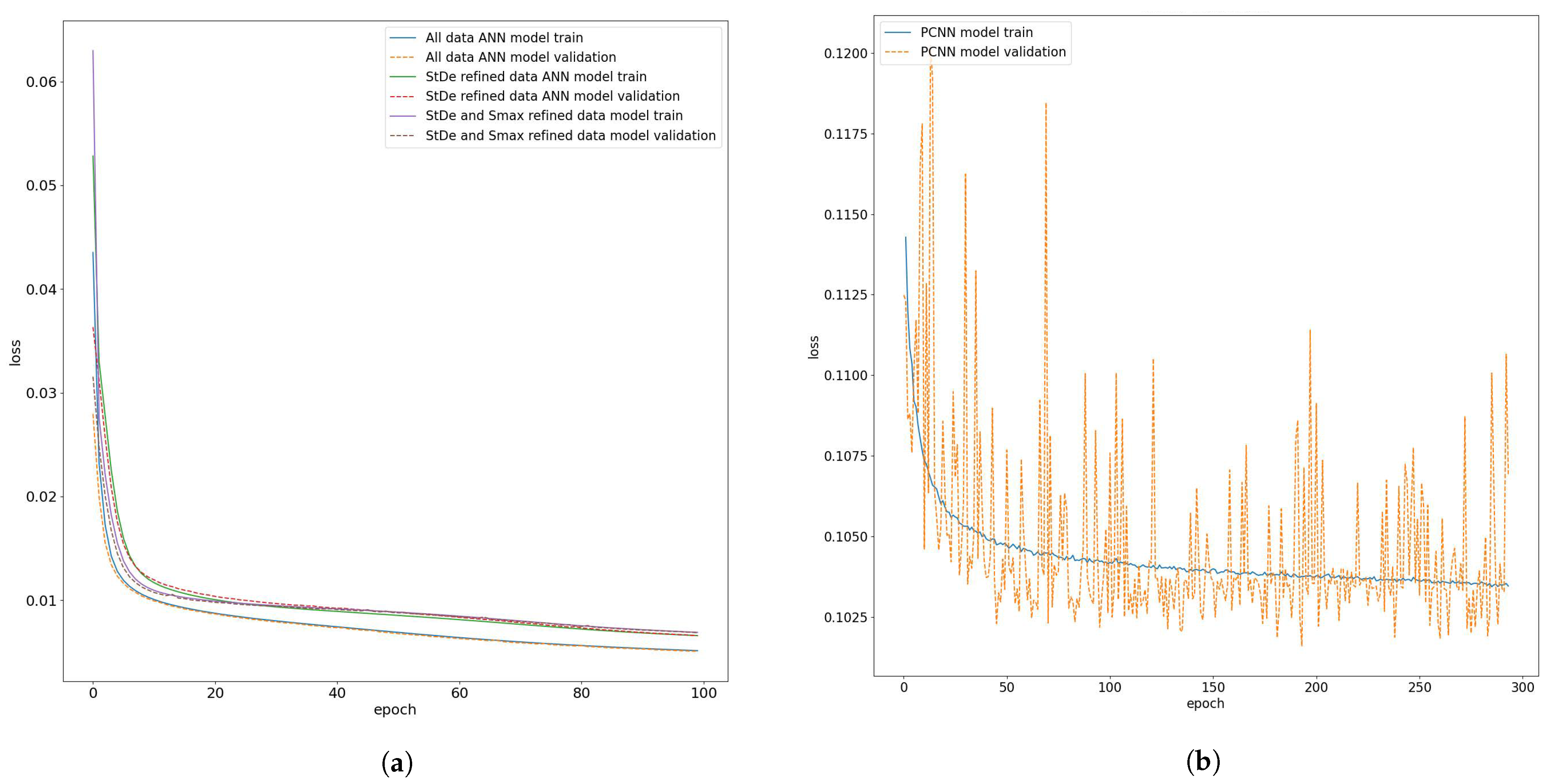
During the training of the ANN and PCNN, several key metrics were saved for evaluation. These metrics included the total loss, mean absolute error (MAE), and mean squared error (MSE) at each epoch for both the training and test stages. For the ANN, the training loss was the same as MSE, but for the PCNN, the loss was a combination of the MSE as well as the loss as calculated in Equation (6). Understanding the training and test loss at each epoch helps determine whether the model fits the data correctly rather than over-fits. The deviation between the validation training loss can be used as a metric to determine over-fitting during the training. A small deviation in between them is expected, while a significantly larger test loss compared to the training loss indicates over-fitting. A comparison of the training loss and test loss for all three ANN models is presented in Figure 2a and the history for the PCNN is presented in Figure 2b. A large decrease in the loss is seen during the initial training phase. The large decrease is a result of back-propagation of the error that makes the neurons adjust their weights aggressively. The loss of the models decreases slowly as the number of epochs increase. The ANN is designed to stop training if there is no improvement in loss for 10 consecutive epochs. However, in all the studied cases, the ANN went to completion till the number of epochs provided was reached. It can be seen in Figure 2 that the test loss closely followed the trend of the training loss thus, indicating that ANN as well as the PCNN did not over-fit the data. The ANN loss compared to the PCNN was lower due to the definition of loss for the PCNN, but the loss is not the sole indicator for comparing the performance of the ANN to the PCNN. The final validation loss for the ANN model was , the refined model was , the and refined model was , while the PCNN had the highest validation loss at .
The performance of the model can be determined by the accuracy with which it predicts the test data. In this case, 10,080 data points were used as test data for evaluations of the models. Figure 3 shows a prediction of the granule size distribution (GSD) by all four models developed. A total of six randomly chosen data points are represented in Figure 3. The predictions of the three neural networks without any physical constraints demonstrated similar behavior. The trends each model follows varies marginally from one another, but it can be seen that the model which were provided with filtered data did not seem to perform better than the ANN model that was fed all the data as input. Thus, it can be we can conclude that the and refined data performed did not have a large effect on the model prediction capabilities. This was also verified by the coefficient of determination or values as the and data filtered model had a of compared to the data refined model with a of , while the all data as input ANN had a higher value of . The performance of the PCNN was comparatively slightly lower than the best performing of the three ANN models with a value of . The prediction of the data points may seem misleading for the PCNN since the GSD predicted by the PCNN was penalized if the growth did not occur in the steady-growth or nucleation growth regime. This meant that the PCNN prediction did not follow a trend similar to that of the other ANN models results and in some cases even the PBM simulation data. However, the positive effect of this physics-based constraint can be seen in Section 4.2, where the PCNN predicts growth regimes with more accuracy than the other ANN models near the boundary conditions. Identifying these regimes is important to identify granules which may not have the desired CQAs required for further downstream processing.
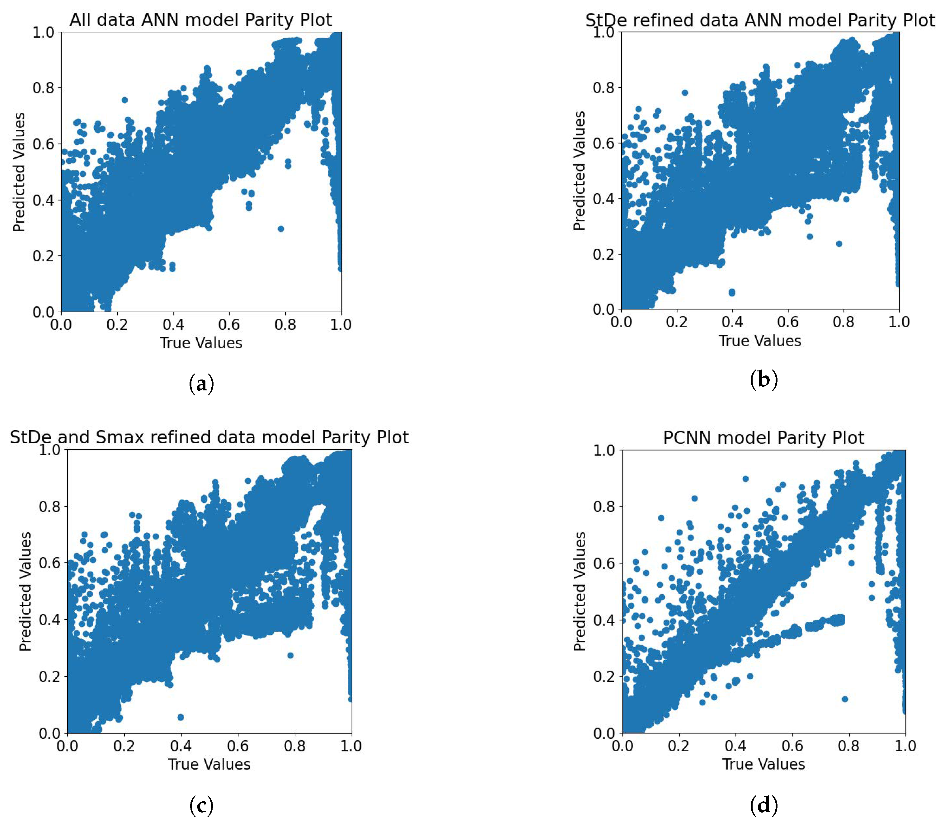
A comparison of the experimental data and predictions from the model can be visualized using parity plots. Figure 4 contains the parity plots which compare the testing data simulated experimental values with the predicted values for all four models developed. The model with a higher number of points closer to the line indicates that the model had a better prediction capability. Figure 4a has the most number of points closer to the aforementioned line, thus having the best prediction capability of the four ANN models. This is in accord with the previous observation of the value. The refining of data with physical laws removes all the points from the PBM data that would violate the steady growth regime boundary conditions, thus providing the corresponding model with less or no bad data points. This clean data in turn reduces the prediction capability of the ANN model. The PCNN in comparison has a lesser number of points lying across the line, since several of the data points violate the steady growth regime for granules. The PCNN does not predict such points but rather attempts to predict the GSD of granules assuming that their growth under a steady state regime. Since the constraint due to the only affects the output value of the granule density and not the GSD, this leads to the predictions deviating. However this constraint helps the PCNN predict quality attributes of the granule growth process better. This has been discussed in more detail in Section 4.2.
4.2. Comparing Artificial Neural Networks and Physics-Constrained Neural Network at Growth Regime Boundary Conditions
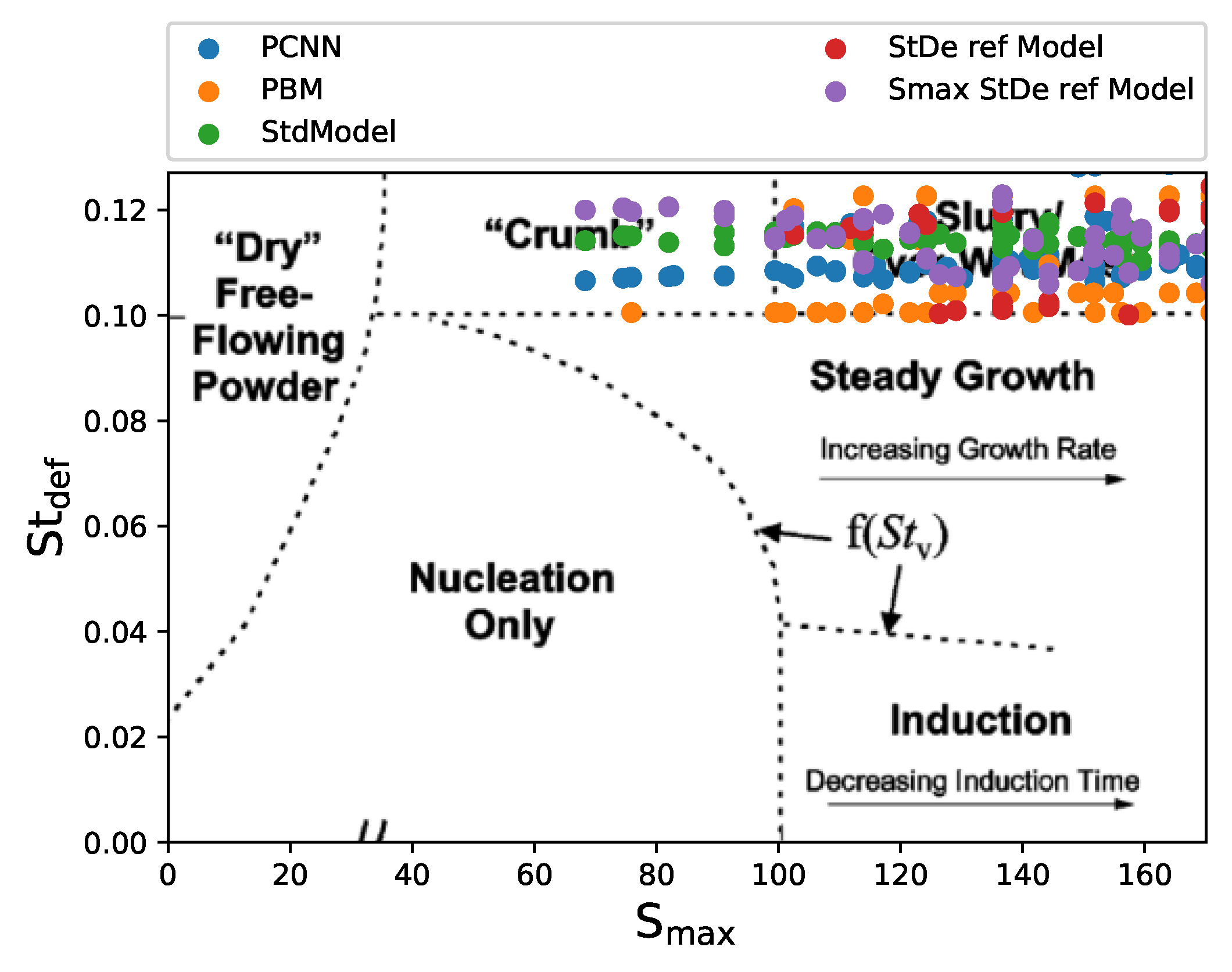
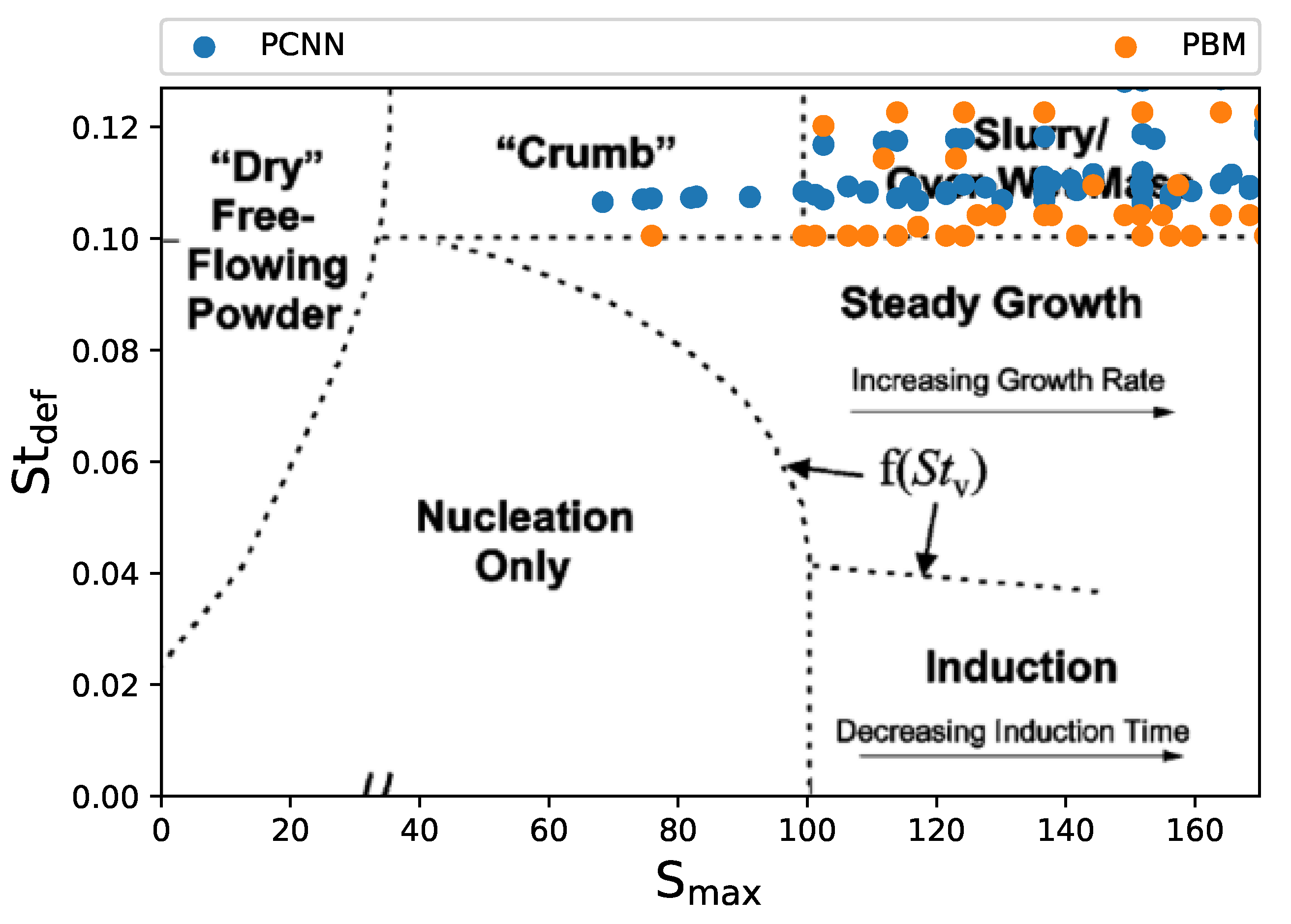
The reliance of the PBM on the kernel rate constants makes its susceptible to changes in the process parameters provided. Sometimes the outputs from the PBM may not reproduce the actual system dynamics accurately [55]. This may lead to the PBM predicting granule growth in the crumb and slurry regime. Identifying these points during prediction is essential for understanding the process dynamics. The data driven may be able to predict the GSD accurately, other critical quality attributes (CQAs) may not be up to specification and the granules may have to be discarded. For this analysis, the outputs from all four models were collected and corresponding and for these points were calculated. These points were then plotted against the regime map developed for high shear wet granulation by [19]. All the data points where the test data exceeded the boundary condition of were collected from each of the predictions and plotted in Figure 5. It can be seen from Figure 5 that the ANN model as well as both the data refined models predict growth regime which are not in accord with the test data. The ANN model predicted about 40 points less lie in the regime compared to the test data, whereas the refined model over-predicted these points by 226. On the contrary, the and model under-predicted these points by more than 150. These predictions by the pure data-driven models may lead to more or less failed batches of granulation respectively.
Compared to these pure data-driven models, the PCNN was the most accurate and only deviated from the test data by 10 points. The PCNN had an error of an identifying regime of approximately where as, the other ANN had at least an approximate error of . The highest error in identification was observed for the refined model, which had an error of . The deviation of the prediction in other data refined models can be attributed to the lack points with in the training data. On the other hand, the standard ANN used all the training data and had better predictions, but it still lacked the accuracy of the PCNN since the PCNN was able to identify these points due to the added constraints. Thus, PCNN had the ability to predict the overall granule growth regimes more accurately and can be used to identify batches of granules with undesired growth behavior before further processing occurs. This reduces the amount of inherent risk in the process and can have potential large cost saving benefits in pharmaceutical manufacturing.
4.3. Input Parameters Sensitivity Analysis
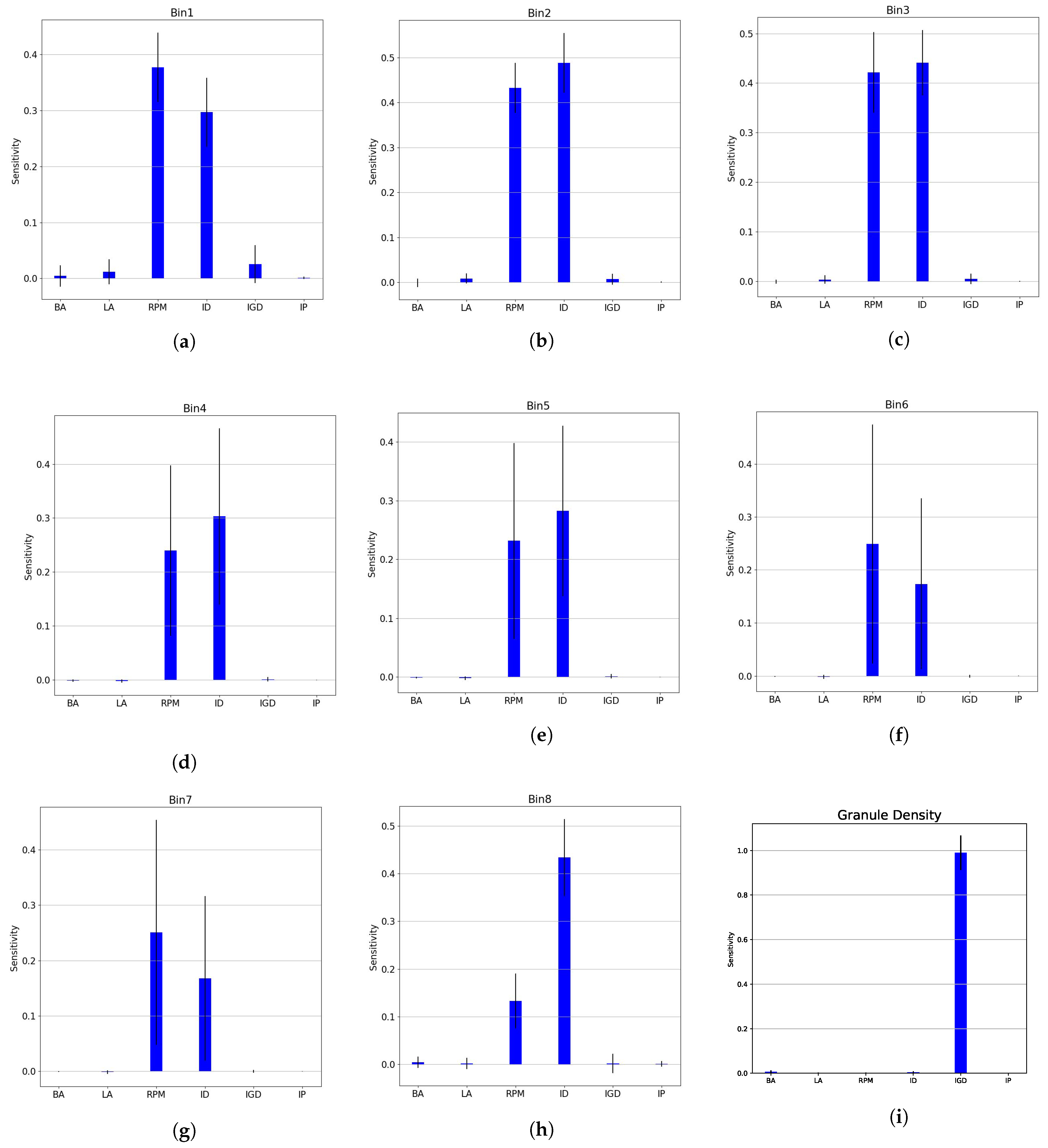
Risk assessment during a process development in pharmaceutical manufacturing is essential and can lead to the understanding and linkage of process parameters and material attributes on the product CQAs [11]. Figure 6 contains nine subplots with the sensitivity of each output with respect to the input process parameters. The blue bars represent the first order sensitivity with the black lines marking the confidence interval. The closer the value is to 1, the higher the effect the input parameter has on the outputs. Figure 6a–h show the effect of the process parameters on the GSD whereas Figure 6i shows their effect on the granule density. The impeller diameter (ID) and the rotation speed of the impeller (RPM) seem to have the highest impact on the PCNN’s prediction of GSD. Smaller effects of the initial granule density (IGD) and Liquid Amount (LA) can be seen in bins with smaller sieve cuts. The final bin, which mainly consists of large particles, shows ID having a more dominating effect followed by batch amount(BA) and other parameters having a smaller impact. The interchangeable nature of the sensitivity between RPM and ID seen here is one added advantage of using neural networks as they can identify very complex relationships within the dataset. In Figure 6i, IGD seems to have a large dominating effect on the final granule density prediction. Other process parameters do not show a major effect in the granule density.
5. Conclusions
In this work, a framework was presented in which physics-based constrains were introduced inside a neural network for a granulation process. The PCNN used was bench-marked against pure data-driven neural network and it showed improved predictions on identifying granule growth regimes during the granulation process. The PCNN excelled at identifying granule batches with bad growth behavior and was able to identify these bad granule growth regimes with a accuracy. This makes the PCNN an important tool for process development and risk assessment. With some modifications, this model could be used in manufacturing for real-time process identificaiton. A sensitivity analysis of the input process parameters was also performed to understand the effect of the inputs on the various outputs of the PCNN. The behavior of the PCNN could be skewed to steady growth regime, which could have been a result of the constraints only applied for a certain type of growth. This model thus can be expanded upon to include more boundary conditions to ensure that the system is more physics aware and mimics experimental data more accurately. The PCNN could be extended to be used with real experimental data instead of simulation data used here in order to mimic real granulation processes better. With the advancement of sensors and data acquisition techniques, this a necessary step in order to have the real-time prediction of complex particulate processes.
Author Contributions
Conceptualization, C.S. and R.R.; methodology, C.S.; software, C.S.; validation, C.S. and R.R.; formal analysis, C.S.; investigation, C.S.; resources, R.R.; data curation, C.S.; writing—original draft preparation, C.S.; writing—review and editing, C.S. and R.R.; visualization, C.S.; supervision, R.R.; project administration, R.R.; funding acquisition, R.R. All authors have read and agreed to the published version of the manuscript.
Funding
This research was funded by US Food and Drug Administration through grant DHHS-FDA-U01FD006487.
Data Availability Statement
Source code and input scripts for reproduction of the experiments can be found at: https://github.com/csampat/PCNN_PBM (accessed on 19 April 2021).
Acknowledgments
The authors would also like to acknowledge Anik Chaturbedi and Indu Muthancheri for their help with development of the PBM code and inputs.
Conflicts of Interest
The authors declare no conflict of interest.
Appendix A. PBM Equations
The PBM consisted of two compartments, one to account for liquid distribution inside the spray zone and the other to account for the bulk of the powder inside the high shear granulator. The model lumped the liquid and gas volumes and this lumped one-dimensional PBM can be represented as follows:
Here, represents the number of particle with solid volume at time t in the compartment i or j, where , or indicate the two different compartments. and are the total liquid volume and gas volume respectively present in the solid volume of in compartment i. and represent the liquid and gas volume of each particle having solid volume . is the rate of particle transfer between the two compartments and , are the rate of particle transfer between different size classes due to aggregation and breakage rate processes respectively.
Appendix B. Comparing Regime Predictions for PBM and PCNN
Figure A1 illustrates the comparison of the PCNN predictions with the PBM data. It can be observed that the prediction and data are in close accord.
Figure A1.
Comparing the PCNN predictions with PBM data with and it can be observed that the PCNN is more accurate in identifying the undesired granule growth regime
Figure A1.
Comparing the PCNN predictions with PBM data with and it can be observed that the PCNN is more accurate in identifying the undesired granule growth regime

References
- Chand, S.; Davis, J. What is Smart Manufacturing? Time Magazine, 7 July 2010. [Google Scholar]
- Venkatasubramanian, V. The promise of artificial intelligence in chemical engineering: Is it here, finally? AIChE J. 2019, 65, 466–478. [Google Scholar] [CrossRef]
- Pham, D.T.; Afify, A.A. Machine-learning techniques and their applications in manufacturing. Proc. Inst. Mech. Eng. Part B J. Eng. Manuf. 2005, 219, 395–412. [Google Scholar] [CrossRef]
- GE. Deep Machine Learning: GE and BP Will Connect Thousands of Subsea Oil Wells to the Industrial Internet. 2015. Available online: https://www.ge.com/news/reports/deep-machine-learning-ge-and-bp-will-connect-2 (accessed on 23 September 2020).
- Huang, E.; Xu, J.; Zhang, S.; Chen, C.H. Multi-fidelity Model Integration for Engineering Design. Procedia Comput. Sci. 2015, 44, 336–344. [Google Scholar] [CrossRef] [Green Version]
- Raissi, M.; Karniadakis, G.E. Hidden physics models: Machine learning of nonlinear partial differential equations. J. Comput. Phys. 2018, 357, 125–141. [Google Scholar] [CrossRef] [Green Version]
- Seville, J.; Tüzün, U.; Clift, R. Processing of Particulate Solids; Springer Science & Business Media: Berlin/Heidelberg, Germany, 2012; Volume 9. [Google Scholar]
- Litster, J.; Bogle, I.D.L. Smart Process Manufacturing for Formulated Products. Engineering 2019, 5, 1003–1009. [Google Scholar] [CrossRef]
- Litster, J. Design and Processing of Particulate Products; Cambridge University Press: Cambridge, UK, 2016. [Google Scholar]
- Rogers, A.J.; Hashemi, A.; Ierapetritou, M.G. Modeling of particulate processes for the continuous manufacture of solid-based pharmaceutical dosage forms. Processes 2013, 1, 67–127. [Google Scholar] [CrossRef] [Green Version]
- US-FDA. Guidance for Industry Q8(R2) Pharmaceutical Development; ICH: Silver Spring, MD, USA, 2009.
- Azarpour, A.; Borhani, T.N.; Alwi, S.R.W.; Manan, Z.A.; Mutalib, M.I.A. A generic hybrid model development for process analysis of industrial fixed-bed catalytic reactors. Chem. Eng. Res. Des. 2017, 117, 149–167. [Google Scholar] [CrossRef]
- Chen, Y.; Ierapetritou, M. A framework of hybrid model development with identification of plant-model mismatch. AIChE J. 2020, 66, e16996. [Google Scholar] [CrossRef]
- Katare, S.; Caruthers, J.M.; Delgass, W.N.; Venkatasubramanian, V. An Intelligent System for Reaction Kinetic Modeling and Catalyst Design. Ind. Eng. Chem. Res. 2004, 43, 3484–3512. [Google Scholar] [CrossRef]
- Raissi, M.; Perdikaris, P.; Karniadakis, G.E. Physics-informed neural networks: A deep learning framework for solving forward and inverse problems involving nonlinear partial differential equations. J. Comput. Phys. 2019, 378, 686–707. [Google Scholar] [CrossRef]
- Jagtap, A.D.; Kawaguchi, K.; Karniadakis, G.E. Adaptive activation functions accelerate convergence in deep and physics-informed neural networks. J. Comput. Phys. 2020, 404, 109136. [Google Scholar] [CrossRef] [Green Version]
- Zhu, Y.; Zabaras, N.; Koutsourelakis, P.S.; Perdikaris, P. Physics-constrained deep learning for high-dimensional surrogate modeling and uncertainty quantification without labeled data. J. Comput. Phys. 2019, 394, 56–81. [Google Scholar] [CrossRef] [Green Version]
- Iveson, S.M.; Litster, J.D.; Hapgood, K.; Ennis, B.J. Nucleation, growth and breakage phenomena in agitated wet granulation processes: A review. Powder Technol. 2001, 117, 3–39. [Google Scholar] [CrossRef]
- Iveson, S.M.; Wauters, P.A.; Forrest, S.; Litster, J.D.; Meesters, G.M.; Scarlett, B. Growth regime map for liquid-bound granules: Further development and experimental validation. Powder Technol. 2001, 117, 83–97. [Google Scholar] [CrossRef]
- Cameron, I.T.; Wang, F.Y.; Immanuel, C.D.; Stepanek, F. Process systems modelling and applications in granulation: A review. Chem. Eng. Sci. 2005, 60, 3723–3750. [Google Scholar] [CrossRef]
- Ramkrishna, D.; Singh, M.R. Population balance modeling: Current status and future prospects. Annu. Rev. Chem. Biomol. Eng. 2014, 5, 123–146. [Google Scholar] [CrossRef] [PubMed] [Green Version]
- Barrasso, D.; Hagrasy, A.E.; Litster, J.; Ramachandran, R. Multi-dimensional population balance model development and validation for a twin screw granulation process. Powder Technol. 2015, 270, 612–621. [Google Scholar] [CrossRef]
- Barrasso, D.; Walia, S.; Ramachandran, R. Multi-component population balance modeling of continuous granulation processes: A parametric study and comparison with experimental trends. Powder Technol. 2013, 241, 85–97. [Google Scholar] [CrossRef]
- Barrasso, D.; Tamrakar, A.; Ramachandran, R. Model Order Reduction of a Multi-scale PBM-DEM Description of a Wet Granulation Process via ANN. Procedia Eng. 2015, 102, 1295–1304. [Google Scholar] [CrossRef] [Green Version]
- Chaudhury, A.; Kapadia, A.; Prakash, A.V.; Barrasso, D.; Ramachandran, R. An extended cell-average technique for a multi-dimensional population balance of granulation describing aggregation and breakage. Adv. Powder Technol. 2013, 24, 962–971. [Google Scholar] [CrossRef]
- Immanuel, C.D.; Doyle, F.J. Solution technique for a multi-dimensional population balance model describing granulation processes. Powder Technol. 2005, 156, 213–225. [Google Scholar] [CrossRef]
- Gunawan, R.; Fusman, I.; Braatz, R.D. Parallel high-resolution finite volume simulation of particulate processes. AIChE J. 2008, 54, 1449–1458. [Google Scholar] [CrossRef]
- Prakash, A.V.; Chaudhury, A.; Barrasso, D.; Ramachandran, R. Simulation of population balance model-based particulate processes via parallel and distributed computing. Chem. Eng. Res. Des. 2013, 91, 1259–1271. [Google Scholar] [CrossRef]
- Bettencourt, F.E.; Chaturbedi, A.; Ramachandran, R. Parallelization methods for efficient simulation of high dimensional population balance models of granulation. Comput. Chem. Eng. 2017, 107, 158–170. [Google Scholar] [CrossRef]
- Prakash, A.V.; Chaudhury, A.; Ramachandran, R. Parallel simulation of population balance model-based particulate processes using multicore {CPUs} and {GPUs}. Model. Simul. Eng. 2013, 2013, 475478. [Google Scholar] [CrossRef] [Green Version]
- Sampat, C.; Baranwal, Y.; Ramachandran, R. Accelerating multi-dimensional population balance model simulations via a highly scalable framework using GPUs. Comput. Chem. Eng. 2020, 140, 106935. [Google Scholar] [CrossRef]
- Sampat, C.; Bettencourt, F.; Baranwal, Y.; Paraskevakos, I.; Chaturbedi, A.; Karkala, S.; Jha, S.; Ramachandran, R.; Ierapetritou, M. A parallel unidirectional coupled DEM-PBM model for the efficient simulation of computationally intensive particulate process systems. Comput. Chem. Eng. 2018, 119, 128–142. [Google Scholar] [CrossRef]
- McCulloch, W.S.; Pitts, W. A logical calculus of the ideas immanent in nervous activity. Bull. Math. Biophys. 1943, 5, 115–133. [Google Scholar] [CrossRef]
- Fletcher, L.; Katkovnik, V.; Steffens, F.E.; Engelbrecht, A.P. Optimizing the number of hidden nodes of a feedforward artificial neural network. In Proceedings of the 1998 IEEE International Joint Conference on Neural Networks Proceedings, IEEE World Congress on Computational Intelligence (Cat. No.98CH36227), Anchorage, AK, USA, 4–9 May 1998; Volume 2, pp. 1608–1612. [Google Scholar]
- Baydin, A.G.; Pearlmutter, B.A.; Radul, A.A.; Siskind, J.M. Automatic differentiation in machine learning: A survey. J. Mach. Learn. Res. 2018, 18, 1–43. [Google Scholar]
- Murtoniemi, E.; Yliruusi, J.; Kinnunen, P.; Merkku, P.; Leiviskä, K. The advantages by the use of neural networks in modelling the fluidized bed granulation process. Int. J. Pharm. 1994, 108, 155–164. [Google Scholar] [CrossRef]
- Aksu, B.; Paradkar, A.; de Matas, M.; Özgen, Ö.; Güneri, T.; York, P. A quality by design approach using artificial intelligence techniques to control the critical quality attributes of ramipril tablets manufactured by wet granulation. Pharm. Dev. Technol. 2013, 18, 236–245. [Google Scholar] [CrossRef]
- Pishnamazi, M.; Ismail, H.Y.; Shirazian, S.; Iqbal, J.; Walker, G.M.; Collins, M.N. Application of lignin in controlled release: Development of predictive model based on artificial neural network for API release. Cellulose 2019, 26, 6165–6178. [Google Scholar] [CrossRef]
- Ismail, H.Y.; Singh, M.; Darwish, S.; Kuhs, M.; Shirazian, S.; Croker, D.M.; Khraisheh, M.; Albadarin, A.B.; Walker, G.M. Developing ANN-Kriging hybrid model based on process parameters for prediction of mean residence time distribution in twin-screw wet granulation. Powder Technol. 2019, 343, 568–577. [Google Scholar] [CrossRef]
- Shirazian, S.; Kuhs, M.; Darwish, S.; Croker, D.; Walker, G.M. Artificial neural network modelling of continuous wet granulation using a twin-screw extruder. Int. J. Pharm. 2017, 521, 102–109. [Google Scholar] [CrossRef]
- Rantanen, J.; Räsänen, E.; Antikainen, O.; Mannermaa, J.P.; Yliruusi, J. In-line moisture measurement during granulation with a four-wavelength near-infrared sensor: An evaluation of process-related variables and a development of non-linear calibration model. Chemom. Intell. Lab. Syst. 2001, 56, 51–58. [Google Scholar] [CrossRef]
- Van Hauwermeiren, D.; Stock, M.; De Beer, T.; Nopens, I. Predicting Pharmaceutical Particle Size Distributions Using Kernel Mean Embedding. Pharmaceutics 2020, 12, 271. [Google Scholar] [CrossRef] [PubMed] [Green Version]
- Barrasso, D.; Tamrakar, A.; Ramachandran, R. A reduced order PBM–ANN model of a multi-scale PBM–DEM description of a wet granulation process. Chem. Eng. Sci. 2014, 119, 319–329. [Google Scholar] [CrossRef]
- Liu, D.; Wang, Y. A Dual-Dimer Method for Training Physics-Constrained Neural Networks with Minimax Architecture. arXiv 2020, arXiv:2005.00615. [Google Scholar]
- Goswami, S.; Anitescu, C.; Chakraborty, S.; Rabczuk, T. Transfer learning enhanced physics informed neural network for phase-field modeling of fracture. Theor. Appl. Fract. Mech. 2020, 106, 102447. [Google Scholar] [CrossRef] [Green Version]
- Sahli Costabal, F.; Yang, Y.; Perdikaris, P.; Hurtado, D.E.; Kuhl, E. Physics-Informed Neural Networks for Cardiac Activation Mapping. Front. Phys. 2020, 8, 42. [Google Scholar] [CrossRef] [Green Version]
- Chaturbedi, A.; Bandi, C.K.; Reddy, D.; Pandey, P.; Narang, A.; Bindra, D.; Tao, L.; Zhao, J.; Li, J.; Hussain, M.; et al. Compartment based population balance model development of a high shear wet granulation process via dry and wet binder addition. Chem. Eng. Res. Des. 2017, 123, 187–200. [Google Scholar] [CrossRef]
- Chollet, F. Keras. 2015. Available online: https://github.com/fchollet/keras (accessed on 19 April 2021).
- Abadi, M.; Agarwal, A.; Barham, P.; Brevdo, E.; Chen, Z.; Citro, C.; Corrado, G.S.; Davis, A.; Dean, J.; Devin, M.; et al. TensorFlow: Large-Scale Machine Learning on Heterogeneous Systems. 2015. Available online: https://www.tensorflow.org/ (accessed on 19 April 2021).
- LeCun, Y.A.; Bottou, L.; Orr, G.B.; Müller, K.R. Efficient BackProp. In Neural Networks: Tricks of the Trade, 2nd ed.; Montavon, G., Orr, G.B., Müller, K.R., Eds.; Springer: Berlin/Heidelberg, Germany, 2012; pp. 9–48. [Google Scholar]
- Dhenge, R.M.; Cartwright, J.J.; Hounslow, M.J.; Salman, A.D. Twin screw wet granulation: Effects of properties of granulation liquid. Powder Technol. 2012, 229, 126–136. [Google Scholar] [CrossRef]
- Sobol, I.M. Sensitivity analysis for non-linear mathematical models. Math. Model. Comput. Exp. 1993, 1, 407–414. [Google Scholar]
- Herman, J.; Usher, W. SALib: An open-source Python library for Sensitivity Analysis. J. Open Source Softw. 2017, 2, 97. [Google Scholar] [CrossRef]
- Saltelli, A.; Tarantola, S.; Chan, K.S. A quantitative model-independent method for global sensitivity analysis of model output. Technometrics 1999, 41, 39–56. [Google Scholar] [CrossRef]
- Chaudhury, A.; Barrasso, D.; Pandey, P.; Wu, H.; Ramachandran, R. Population balance model development, validation, and prediction of CQAs of a high-shear wet granulation process: Towards QbD in drug product pharmaceutical manufacturing. J. Pharm. Innov. 2014, 9, 53–64. [Google Scholar] [CrossRef]
Figure 1.
The algorithm used to determine the optimized weights and biases inside the PCNN.

Figure 2.
Comparing the training and test loss of the three ANNs and PCNN during training. (a) The training loss of the three ANNs seems to be similar, which the normal ANN having a lower loss. (b) The PCNN model has a higher loss compared to the other ANN model due the added regularization of the boundary condition loss. In both plots, the training loss is represented as solid lines while, the dotted lines illustrate the test loss at each epoch.

Figure 3.
Each subplot corresponds to one simulated experimental result and the four model predictions are compared in the plot. A toal of six points at random were chosen for this plot from the test data set for comparison. The blue solid line represents the model prediction for the pure ANN model, the yellow line represents the model prediction for the refined data model, and the green line represents the model prediction of the and . The blue solid line represents the prediction for the PCNN model. The blue dots represent the simulated experimental results. The performance of all four models seems to be similar.

Figure 4.
Parity plot for the three ANN models and the PCNN model. The granule density and GSD predictions by each of these models is compared with the test dataset of 10,800 simulated experimental points. The data refined models in subfigure (b,c) seem to perform worse than the all data ANN model in subfigure (a) and the PCNN model in subfigure (d).

Figure 5.
Comparing the predictions from all 4 model with the test data (PBM). This plot contains all the points where the predictions indicated . The PCNN performs better than the other data-driven models.
Figure 5.
Comparing the predictions from all 4 model with the test data (PBM). This plot contains all the points where the predictions indicated . The PCNN performs better than the other data-driven models.

Figure 6.
Input parameter sensitivity analysis for the physics-constrained neural network. Sub-figures (a–h) represent the effect of the input parameters on the various sieve cuts chosen. The interchangeable effect of RPM and impeller diameter has been identified by the PCNN. Sub-figure (i) indicates that the effect of initial particle size affects the granule density the highest.


Table 1.
Bounds chosen for the input variables sensitivity analysis.
| Input Parameter | Minimum Value | Maximum Value |
|---|---|---|
| Batch amount (kg) | 800 | 2000 |
| Liquid amount (kg) | 600 | 1200 |
| RPM | 100 | 600 |
| Impeller diameter (m) | ||
| Initial granule density (kg/m) | 100 | 600 |
| Initial porosity |
Table 2.
Values of hyperparameters used for the three ANN models and the PCNN.
| Hyperparameter | ANN Value | PCNN Value |
|---|---|---|
| No. of hidden layers | 2 | 3 |
| Neurons in each hidden layer | 16 | 16 |
| Optimizer algorithm | Adam | Adam |
| Optimizer learning rate | ||
| No. of epochs | 200 | 300 |
| Regularization constant | ||
| Hidden layer activation function | ‘tanh’ | ‘tanh’ |
| Last layer activation function | ‘tanh’ | ‘tanh’ |
Publisher’s Note: MDPI stays neutral with regard to jurisdictional claims in published maps and institutional affiliations. |
© 2021 by the authors. Licensee MDPI, Basel, Switzerland. This article is an open access article distributed under the terms and conditions of the Creative Commons Attribution (CC BY) license (https://creativecommons.org/licenses/by/4.0/).
Share and Cite
MDPI and ACS Style
Sampat, C.; Ramachandran, R. Identification of Granule Growth Regimes in High Shear Wet Granulation Processes Using a Physics-Constrained Neural Network. Processes 2021, 9, 737. https://doi.org/10.3390/pr9050737
AMA Style
Sampat C, Ramachandran R. Identification of Granule Growth Regimes in High Shear Wet Granulation Processes Using a Physics-Constrained Neural Network. Processes. 2021; 9(5):737. https://doi.org/10.3390/pr9050737
Chicago/Turabian StyleSampat, Chaitanya, and Rohit Ramachandran. 2021. "Identification of Granule Growth Regimes in High Shear Wet Granulation Processes Using a Physics-Constrained Neural Network" Processes 9, no. 5: 737. https://doi.org/10.3390/pr9050737
Note that from the first issue of 2016, this journal uses article numbers instead of page numbers. See further details here.