A Comparative Study of Linear, Random Forest and AdaBoost Regressions for Modeling Non-Traditional Machining

Abstract

Non-traditional machining (NTM) has gained significant attention in the last decade due to its ability to machine conventionally hard-to-machine materials. However, NTMs suffer from several disadvantages such as higher initial cost, lower material removal rate, more power consumption, etc. NTMs involve several process parameters, the appropriate tweaking of which is necessary to obtain economical and suitable results. However, the costly and time-consuming nature of the NTMs makes it a tedious and expensive task to manually investigate the appropriate process parameters. The NTM process parameters and responses are often not linearly related and thus, conventional statistical tools might not be enough to derive functional knowledge. Thus, in this paper, three popular machine learning (ML) methods (viz. linear regression, random forest regression and AdaBoost regression) are employed to develop predictive models for NTM processes. By considering two high-fidelity datasets from the literature on electro-discharge machining and wire electro-discharge machining, case studies are shown in the paper for the effectiveness of the ML methods. Linear regression is observed to be insufficient in accurately mapping the complex relationship between the process parameters and responses. Both random forest regression and AdaBoost regression are found to be suitable for predictive modelling of NTMs. However, AdaBoost regression is recommended as it is found to be insensitive to the number of regressors and thus is more readily deployable.

1. Introduction

Machining is an essential function for the manufacturing of products and components. Traditionally, all the methods used for machining or surface finishing like cutting, grinding and milling are the processes where hardened tools are used for the comparatively soft workpiece. In these processes, the workpiece is always comparatively weaker than the tool. But in the recent past, many machining processes have been used that don’t rely on traditional machining processes and have been extensively used by different industries. Hence these methods were called non-traditional machining (NTM). In NTM, electric discharge machining (EDM) has played an important role. It is an NTM where an electric spark is used to erode material immersed in dielectric fluid. It works with electrically conductive material [1]. The principle behind EDM is the ability to control sparks to erode materials. The unique feature of EDM is its ability to machine the shape and depth of parts which are impossible with traditional machining processes [2]. Thus, EDM is a precise, cutting-edge machining technique that provides a better surface finish even working with the hardened material. Joseph Priestly first observed the possibility of machining by metal erosion in 1770, and further, B.R. Lazarenko and N.I. Lazarenko inadvertently found out that erosion of tungsten could be reduced if the metal is immersed in a dielectric fluid, which led to the invention of the first EDM machine [3]. The dielectric fluid being used is an electrical insulator that helps in controlling the arc discharge. The dielectric fluid is also used for flushing—a vital technique to remove unwanted metal particles from the operational gaps and assist in machining or erosion. The colour of the spark generated gives the inadequacy of the fluid; if the spark is red, there is inadequate fluid, and if the spark is blue, it shows the sufficiency of the same. Dielectric fluid also helps in cooling the flushing agent [4].

Maintaining the gaps between the electrode and workpiece is a must so that there should not be any physical contact between the electrode and workpiece. If the contact happens between the two, the tool may damage and can also damage the workpiece. To maintain such a gap between them, a servomechanism is used, which helps in maintaining the proper distance between the electrode and the workpiece.

In recent years, researchers have made significant efforts to measure the performance characteristics of EDM. Machining performance of EDM can be characterized by the different parameters like material removal rate (MRR), tool wear rate (TWR), radial overcut (ROC), surface roughness (SR), etc. The controlling process parameter such as voltage, current, pulse-on time and pulse-off time plays an important role in characterizing the machining performance parameters such as MRR, TWR, ROC and SR. To increase the machining efficiency, erosion of the workpiece must be maximized and TWR must be minimized [5]. It has been reported that MRR and SR increase with an increase in pulse-on time and decrease with an increase in pulse-off time [6]. An increase in current leads to an increase in energy sparks which causes the melting of the surface to create a poor surface finish [7].

In NTM processes, the quantitative relationship between the operating parameters and controlling input parameters is often required [8]. For this, researchers have used many regression techniques to reduce the error and give the best empirical relationship between all the dependent and independent parameters.

Table 1. Literature on predictive modelling of NTM processes in last 3 years.

Ref.	Year	NTM Process	Predictive Model	Dataset Size	Task
Dinesh et al. [9]	2019	EDM	ANN, RSM	27	Prediction
Thankachan et al. [10]	2019	WEDM	ANN	32	Prediction
Phate and Toney [11]	2019	WEDM	ANN	27	Prediction
Singh et al. [12]	2019	WEDM	SVM	81	Prediction
Kumar and Suresh [13]	2019	EDM	RSM	27	Prediction and optimization
Ulas et al. [14]	2020	WEDM	SVM, EML, WEML	81	Prediction
Shrinivas [15]	2020	EDM	ANN	9	Prediction and optimization
Abhilash and Chakradhar [16]	2020	WEDM	ANN	81	Classification
Abhilash and Chakradhar [17]	2020	WEDM	ANFIS	81	Prediction
Prasad et al. [18]	2020	WEDM	RSM	9	Prediction and optimization
Lalwani et al. [19]	2020	WEDM	ANN, RSM	50	Prediction and optimization
Manikandan et al. [20]	2020	EDM	ANN	27	Prediction and optimization
El-Bahloul [21]	2020	WEDM	ANN, RSM	20	Prediction
Pattnaik and Sutar [22]	2021	WEDM	ANN	9	Prediction
Paturi et al. [23]	2021	WEDM	ANN, SVM	27	Prediction and optimization
Rajamani et al. [24]	2021	LBM	ANFIS	30	Prediction and optimization
Goyal et al. [25]	2021	WEDM	ANFIS	18	Prediction and optimization
Dubey et al. [26]	2021	EDM	RSM	30	Prediction
Gupta [27]	2021	WEDM	RSM	29	Prediction and optimization
Jiang and Yen [28]	2021	WEDM	LSTM	110	Prediction
Gopinath et al. [29]	2021	ECM	RSM	27	Prediction

presents a brief section of literature on predictive modelling of NTM processes from the last three years.

Based on the literature study, it is observed that response surface methodology (RSM) is the most common predictive modelling approach used for NTM processes. Though RSM is easy to deploy, it suffers from the drawback that its form is fixed a priori. Thus, when the data is much more complex or has substantial non-linearity RSM may fail to accurately model the process. In the literature, very few attempts to use machine learning to build predictive models are seen. This lacuna is addressed in this paper by considering three machine learning methods to build regression models to map the NTM process. As case studies, two examples of EDM and WEDM are considered in the paper. The methodology used in the paper is data-driven and thus can be directly adapted for any other NTM process as well.

The rest of the paper is arranged as follows—the next section describes the methods used in the paper. The metrics used to measure the performance of the ML methods is also discussed in Section 2. In Section 3, two different case studies on EDM and WEDM are discussed. Performances of linear regression, random forest and AdaBoost regression are illustrated in the two case studies. In Section 4, conclusions based on the study are discussed.

2. Methodology

2.1. Linear Regression

Linear regression (LR) is a common and well-known method in statistics and machine learning [30]. The regression model has two main objectives—the first one is to establish a positive relationship between two variables if they tend to move together, and the second is to establish a negative relationship if there is an increase in one variable that leads to a decrease in the other. LR is all about the statistically significant relationship between the two or more variables. In general, these variables play two different roles in the regression model. The dependent variable (denoted by $y$) is the value that needs to be predicted or forecasted. The other is the independent variable (denoted by $x$), which explains the importance of other influencing factors. It is called linear because the equation represents a straight line in a bidimensional plot.

The general equation for the linear regression is

$$y=c+mx$$

(1)

where $c$ and $m$ are the $y$-intercepts and the slope, respectively. The equation is representing the best fit line

$$y=mx$$

(2)

In statistics, generally, this equation is being represented as

$$y={\beta }_0+{\beta }_1{x}_1$$

(3)

If $n$ number of predictors ($x_1,x_2,\dots ,x_n$) are present, then the general equation is

$$y={\beta }_0+{\beta }_1{x}_1+{\beta }_2{x}_2+{\beta }_3{x}_n$$

(4)

2.2. Random Forest Regression

Random forest regression (RFR) is a supervised machine learning predictive algorithm that is constructed through the decision tree algorithms. It is a model ensemble technique that constructs the aggregations of models and improves test accuracy while reducing the costs associated with storing, training and getting inferences from multiple models. Random forest is one of the famous ensemble methods being used for regression. In this ensemble method, many decision trees are being trained, hence it is called a forest, and then the average of each prediction tree becomes the output of the random forest. It is based on the bagging and random subspace method. Bagging, or bootstrapping, is all about training each learner on a different data set. In a random forest, multiple trees are built from the dataset parallelly, and none of the trees is dependent on another tree. Hence it is also called a parallel process [30]. The main benefit of using random forest is that it requires less training time and has high accuracy.

$$\mathrm{Random} \mathrm{forest} \mathrm{prediction}=\frac{1}{K}{\displaystyle \sum }_{k=1}^K{h}_k\left(x\right)$$

(5)

where $K$ is the number of independent regression trees created for the bootstrap samples with input vector x. $h_k\left(x\right)$ is the mean of predictions made by $K$ regression trees.

The mean squared error for out-of-bag data (OOB) dataset is calculated as,

$$MS{E}_{OOB}=\frac{1}{n}{\displaystyle \sum }_{i=i}^n{(y_i-{\overline{y_i}}_{OOB})}^2$$

(6)

where $y_i$ and ${\overline{y_i}}_{OOB}$ are the ith prediction and the mean of ith prediction from all the trees.

The coefficient of determination for out-of-bag data (OOB) dataset is calculated as,

$$R^2{}_{OOB}=1-MS{E}_{OOB}/Va{r}_y$$

(7)

where $Va{r}_y$ is the total variance of the output parameter.

2.3. Adaptive Boosting Regression

Adaptive Boosting Regression (ABR) is a machine learning sequential ensemble technique used to combine several weak learners randomly from the dataset to make a strong learner. The weak learners are formed by applying the machine learning algorithms. During every training dataset, weight is assigned to each sample observation, and these weights are being used to learn each hypothesis. The false predictions are being identified and further assigned to the next base learner with high weight on this incorrect prediction. The exact process is being repeated until the algorithm can correctly classify the output. In regression, the output of an instant is not correct or incorrect but has an absolute value error that may be an arbitrary constant. The median, or the weighted average, is being used for the ensemble prediction of the individual base learner [30].

Table 2. Advantages and disadvantages of the LR, RFR and ABR.

Algorithm	Advantages	Disadvantages
LR	Simple to implement. Easy to interpret. Perfect fitting on linearly separable datasets. Overfitting can be reduced by regularization.	Prone to underfitting. Outliers have large effect. Boundaries are linear. Assumes the data is independent.
RFR	Efficient in handling non-linear parameters. RFR reduces overfitting in decision trees. Can solve both classification and regression.	Can be large, making pruning necessary. Higher training time than decision trees. Change greatly with small change in data.
ABR	Fast, easy to use and easy to program. Reduces bias and variance. Versatile, can handle both text and numeric data.	Sensitive to outliers. Vulnerable to noise. If weak classifier underperforms, the whole model may underperform.

shows the comparative assessment of advantages and disadvantages of the three ML regression methods considered in this study.

3. Results and Discussion

3.1. Case Study 1: EDM Machining Parameter Estimation

3.1.1. Experimental Background

An experimental dataset on EDM machining parameters by using the central composite design reported by Soundhar et al. [31] is considered in this case study. Titanium alloy (Ti–13Zr–13Nb), i.e., TZN, was used as the work material for EDM machining. TZN has high tensile strength and toughness even at high temperatures. The benefit of using TZN is that it is light in weight, has corrosion resistance properties and can resist very high temperatures. TZN is generally used for medical purposes in hip and knee replacement for the orthopedic implant. TZN alloy has inferior machining ability as it is responsible for high TWR, low MRR and poor SR. To overcome these problems, EDM has been chosen for the machining to get the required output.

Production of TZN can be done using different processes like the blended elemental method, cold uniaxial pressing, cold isostatic pressing and vacuum sintering. Soundhar et al. [31] used a hydrated-dehydrated process for making titanium powder. The detailed method followed by Soundhar et al. [31] is as follows—titanium powder was produced using a vertical furnace at a temperature of 500 °C and timing of 3 h with positive pressure. Further on, at ideal room temperature, the hydrate was granulated in a niobium container under a vacuum of 10-2 torr. Zirconium and niobium were being produced with a similar process at a temperature of 800 °C. The hydrate method was being used to reduce cost and produce an increased sintering rate. Further on, the powder was weighed in a lot of 4 g and mixed using a double cone blender in fifteen minutes. After mixing, cold uniaxial pressing was performed at 60 MPa in a steel die cylinder having 15 mm diameter without lubricants. Cold isostatic process press is used to pressurize the specimen at 350 MPa for a duration of 30 s. The specimen was encapsulated under a vacuum of 10-2 torr in a flexible rubber mould. Further sintering was done in a niobium container at 10-7 torr and 900–1500 °C with a heating rate of 20 °C/min using thermal technology equipment. The specimen was being maintained at a particular temperature for an hour, and the furnace was cooled at room temperature.

For the machining process, TZN alloy of specimen size 20 mm in diameter and length of 35 mm was used by Soundhar et al. [31], and graphite electrode of 10 mm for having higher MRR and lower EWR was used. Commercial grade kerosene was used as a dielectric fluid to flush off the unwanted particle in the EDM. A total of 30 experiments were done using die-sinking EDM (GraceD-6030S). The EWR and MRR were computed using the workpiece’s weight variation and was measured with a digital weight machine [31]. Central composite design was used for the design of experiments. The process parameters chosen were voltage, current, pulse-off time and pulse-on time.

3.1.2. Effect of Process Parameters

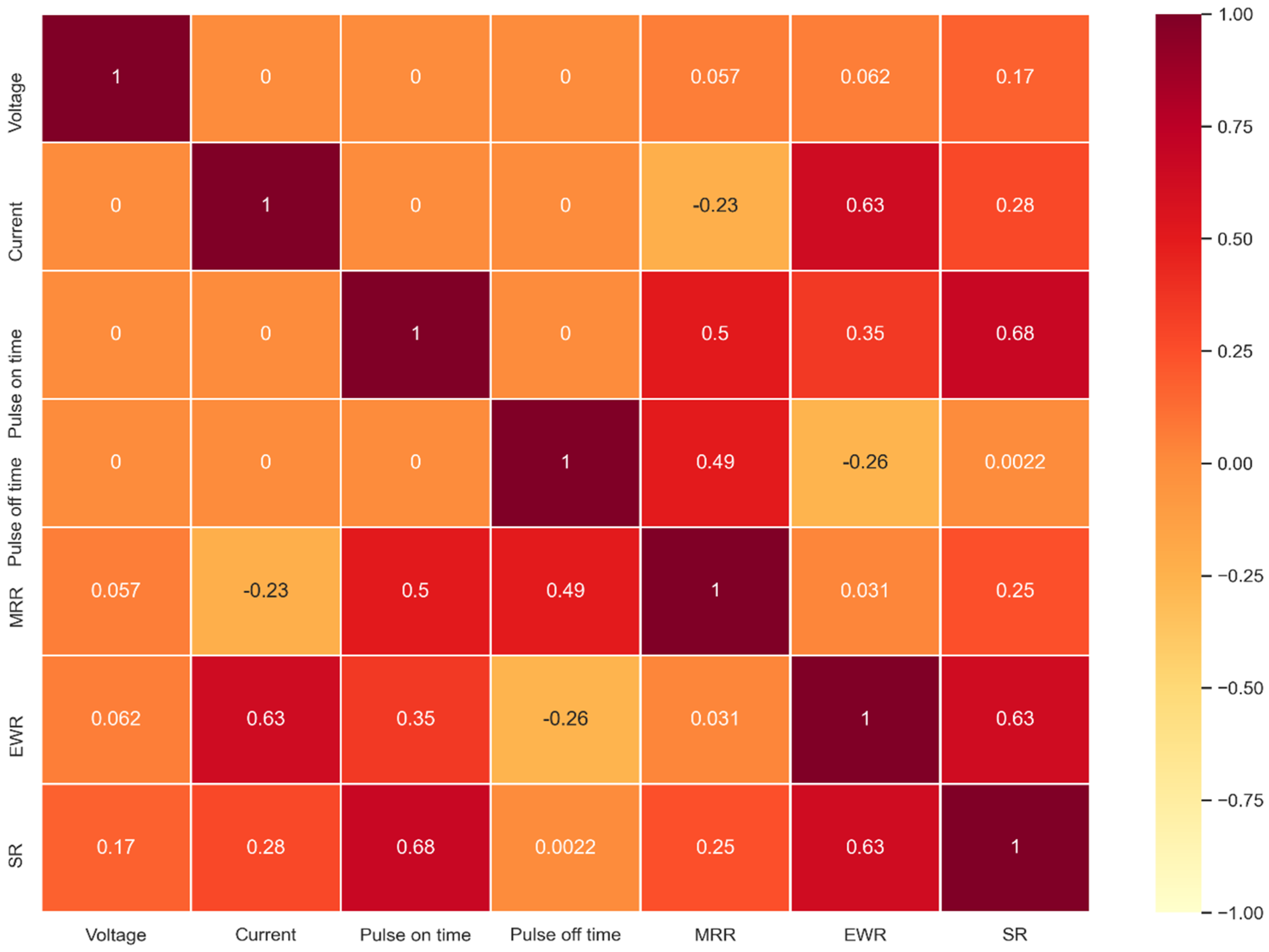
Pearson’s correlation heatmap for the process parameters and the responses is shown in Figure 1. It is observed that no correlation exists amongst the process parameters, indicating a lack of multicollinearity. MRR is observed to have a moderately strong positive correlation with $T_{on}$ and $T_{off}$, whereas EWR has a moderately strong positive correlation with $I$. SR shares a moderately strong positive linear relation with $T_{on}$. All other parameters have a negligible linear relation with MRR, EWR and SR. Thus, ML regression methods beyond the traditional linear regression are necessary for building suitable predictive models.

3.1.3. Linear Regression Models

A linear regression algorithm is used to describe the relationship between the machining factors, i.e., $V$, $I$, $T_{on}$ and $T_{off}$ and MRR. Actual versus predicted responses are plotted in Figure 2. In these figures, two different lines have been shown: one is the identity line (light dash line), and the other is the regression line (dark dash line). The actual MRR value is plotted against the linear regression model-based predictive value of MRR in Figure 2a. Each of the data points represents the $\widehat{y_i}$ value for the corresponding $y_i$. The data points above the identity line come in the category of overprediction and under the line comes in underprediction. The correlation between the $\widehat{y_i}$ and $y_i$ is represented by $R^2$, which is around 55% for the MRR model. $R^2$ shows that how well the linear regression model fits the data. In Figure 2b, $R^2$ for EWR linear regression model is 0.595, which shows that the linear model is inadequate in explaining all the variance in the dataset. Similarly, for the SR model shown in Figure 2c, the $R^2$ is only 56.8%.

Further, the performances of the linear regression models are analyzed by predicted versus residual plots shown in Figure 3. The error terms are assumed to be normally distributed, homoscedastic and independent. The error is being calculated using Equation (8). The residual always sums to zero in the linear regression model. The zeroth line is being shown with the dark line in the figure. A satisfactory residual plot is defined by the maximum number of points close to the zeroth line and very few away from it. The plots in Figure 3 does not show any particular pattern in the scatter of the residuals and hence satisfies the assumption that residuals are independent and normally distributed. From Figure 3b it is observed that except for one outlier all other residuals are within ±0.004. In Figure 3c, though is a random scattering of residuals, the negative residuals are observed to be of larger magnitude than the positive residuals. This indicates that the linear regression SR model has more tendency of overpredicting.

3.1.4. Random Forest Regression Models

In this section, random forest regression models are developed for MRR, EWR and SR. However, since random forest regression models are known to be sensitive to the number of regressors, a sensitivity study is undertaken and reported in

Table 3. Effect of the number of regressors on predictive performance of the MRR random forest model.

Regressor	${\mathit{R}}^2$	MSE	RMSE	MAE	Max. Error	MedAE
100	0.91701	0.00374	0.06117	0.04808	0.12072	0.03753
200	0.94752	0.00316	0.05624	0.04387	0.12998	0.03080
300	0.93336	0.00363	0.06028	0.04641	0.12716	0.03065
400	0.94046	0.00347	0.05894	0.04479	0.11256	0.03042
500	0.93895	0.00337	0.05806	0.04483	0.11371	0.03011
600	0.94517	0.00317	0.05632	0.04338	0.11351	0.03584
700	0.93951	0.00329	0.05735	0.04490	0.11326	0.02921
800	0.94179	0.00334	0.05777	0.04528	0.11697	0.03809
900	0.94648	0.00339	0.05818	0.04555	0.12048	0.03113

. It is observed that the highest $R^2$ and the lowest MSE is recorded for 200 regressors. Thus, 200 regressors are chosen as the optimal for carrying out the rest of the study.

Figure 4 shows the actual versus the random forest regression predicted responses for MRR, EWR and SR. $R^2$ of 94.8%, 74.6% and 86.5%, respectively, are obtained for the MRR, EWR and SR random forest regression models.

Figure 5 illustrates the residual plots for the MRR, EWR and SR random forest regression models. It is observed that for the MRR model the positive residuals are for lower predicted values while the negative residuals are for higher predicted values. This indicates that the model underpredicts higher response values and overpredicts lower MRRs. For both EWR and SR models, an outlier is seen.

3.1.5. AdaBoost Predictive Model

The AdaBoost regression model is a sequential technique where weight is assigned to all the training points. After that, choosing the weak learner and assigning the higher weight continues to get the best prediction. A sensitivity test is carried out to determine the number of regressors for AdaBoost. However, a negligible effect of change in regressors is seen on the performance metrics. Thus, 100 regressors are used for AdaBoost for the rest of the study. Figure 6 shows the relation between the actual and AdaBoost predicted responses. Figure 6a shows a $R^2$ of 95.6% for the MRR model, i.e., an improvement of 1% over the random forest model. The predictive performance of AdaBoost is seen to be poorer than random forest regression for EWR and SR.

Figure 7 illustrates the residual for the AdaBoost regressor models. For the MRR model shown in Figure 7a, the residual pattern is observed to be random. However, from Figure 7b, it is observed that the residuals lie between $\pm$0.004, and a couple of outliers are perhaps responsible for the loss in $R^2$.

3.2. Case Study 2: WEDM of Metal Matrix Composite

3.2.1. Experimental Background

An experimental dataset based on WEDM machining of metal matrix composite, reported by Shandilya et al. [32], is considered in this case study. The design of experimentation of Shandilya et al. [32] is based on Box–Behnken design. WEDM machining was carried out for a rectangular, Al-6061-based metal matrix composite workpiece having a thickness of 6 mm. The input parameters for the machining were voltage, pulse-on time, pulse-off time and wire feed rate to determine the effect on MRR and Kerf. Kerf was measured through a microscope and MRR was calculated by

$$MRR=\frac{M_f-M_i}{\rho t}$$

(8)

where $M_f$ and $M_i$ are the mass of material after and before machining, $\rho$ is the density of workpiece and $t$ is the total time of machining.

3.2.2. Effect of Process Parameters

The effect of process parameters on the MRR and Kerf is investigated using a heatmap plot and depicted in Figure 8. The process parameters show no sign of multicollinearity. No linear trends are observed between the process parameters and the responses. MRR and Kerf seem to be mildly related. MRR is observed to be negatively correlated with voltage, whereas Kerf is positively correlated with voltage. MRR and Kerf share a strong negative correlation between them.

3.2.3. Predictive Modelling of MRR and Kerf

As evident from the lack of strong linear correlations in Figure 8, linear regression algorithm will be insufficient in modelling the complex machining process. In fact, it was found that the linear regression models have poor predictive ability of only 41.5% and 50.7% $R^2$ for MRR and Kerf model, respectively. Due to paucity of space, graphical results for linear regression are not presented for this case study.

Actual versus the predicted responses by random forest regression models are presented in Figure 9. A drastic improvement as compared to the linear regression models is observed. The $R^2$ of the random forest regression models improved by approximately 49% and 43% for MRR and Kerf, respectively. However, still, some large underprediction residuals are present in the MRR model, as observed from Figure 10a.

The AdaBoost predictive regression MMR model is shown in Figure 11a which shows an improvement of approximately 7% over the random forest model. The Kerf model is seen to be of approximately similar predictive power as the random forest model.

From Figure 12, the residuals for the MRR model are concentrated between $\pm$0.4. However, all the errors are reported at the lower MRRs whereas for higher MRRs near-ideal estimation is seen.

4. Conclusions

Non-traditional machining processes find tremendous use in the modern manufacturing sector primarily due to their ability to machine conventionally hard-to-machine materials. These NTMs depend on various technological process parameters that must be carefully calibrated to obtain the desired performance. However, owing to the expensive nature of the physical experiments, it is not always possible to apply a brute force approach to find the best possible combination of process parameters. In real-world situations, even before proceeding to the optimization phase, accurate estimations of the responses must be carried out.

In this paper, two case studies on EDM and WEDM are illustrated to highlight the potential of machine learning in building accurate predictive models. Scatter plots of the process parameters and the responses were used to ascertain the presence or absence of any general trend of association. Correlation heat maps between the various process parameters indicate the lack of any multicollinearity. Also, correlation heat maps between the process parameters and the responses helped in identifying any linear trend in between them.

Three popular ML algorithms, namely linear regression, random forest regression and AdaBoost regression, are considered for the task. Several error metrics are used to highlight the effectiveness of each ML model. Based on the comprehensive evaluation of the two case studies it is observed that though linear regression is simple and quick, it falls short of accurately mapping the complex interaction between the process parameters and the responses. On the other hand, random forest regression and AdaBoost regression showed remarkable accuracy on all the problems. Generally, AdaBoost regression was found to be marginally superior to random forest regression in terms of accuracy. However, the insensitiveness of AdaBoost on the number of regressors makes it a time-saving option. Thus, it can be concluded that by deploying ML predictive models, a fast and inexpensive data-driven surrogate approach to exhaustive experimentation can be established.

One of the limitations of this study is the lack of thorough analysis on the effect of design of experiments (DoE) on such ML systems. This could not be done in this study due to the lack of appropriate datasets in the literature. Though, in this study, two different DoEs called CCD and BBD were used for case study 1 and 2, respectively, no appreciable variation in the ML models was seen with respect to the DoEs, perhaps because both CCD and BBD belong to the same class of DoEs.

As a future scope to this work several other machine learning models such as support vector machining, multi-layer perceptron, Gaussian regression model, etc. will be considered. Studying the uncertainty associated with the NTM processes through ML is also an interesting avenue. Further, it will be interesting to see how these machine learning models perform when deployed in a process optimization scenario. For these, the ML models may be deployed along with metaheuristic algorithms.

References

- Singh, A.; Ghadai, R.K.; Kalita, K.; Chatterjee, P.; Pamučar, D. EDM process parameter optimization for efficient machining of Inconel-718. Facta Univ. Ser. Mech. Eng. 2020, 18, 473–490. [Google Scholar] [CrossRef]
- Salman, Ö.; Kayacan, M.C. Evolutionary programming method for modeling the EDM parameters for roughness. J. Mater. Process. Technol. 2008, 200, 347–355. [Google Scholar] [CrossRef]
- Ganesh, N.; Ghadai, R.K.; Bhoi, A.K.; Kalita, K.; Gao, X.-Z. An Intelligent Predictive Model-Based Multi-Response Optimization of EDM Process. Comput. Modeling Eng. Sci. 2020, 124, 459–476. [Google Scholar] [CrossRef]
- Li, C.; Xu, X.; Li, Y.; Tong, H.; Ding, S.; Kong, Q.; Zhao, L.; Ding, J. Effects of dielectric fluids on surface integrity for the recast layer in high speed EDM drilling of nickel alloy. J. Alloys Compd. 2019, 783, 95–102. [Google Scholar] [CrossRef]
- Majumder, A. Comparative study of three evolutionary algorithms coupled with neural network model for optimization of electric discharge machining process parameters. Proc. Inst. Mech. Eng. Part B J. Eng. Manuf. 2015, 229, 1504–1516. [Google Scholar] [CrossRef]
- Goswami, A.; Kumar, J. Optimization in wire-cut EDM of Nimonic-80A using Taguchi’s approach and utility concept. Eng. Sci. Technol. Int. J. 2014, 17, 236–246. [Google Scholar] [CrossRef] [Green Version]
- Arooj, S.; Shah, M.; Sadiq, S.; Jaffery, S.H.I.; Khushnood, S. Effect of Current in the EDM Machining of Aluminum 6061 T6 and its Effect on the Surface Morphology. Arab. J. Sci. Eng. 2014, 39, 4187–4199. [Google Scholar] [CrossRef]
- Yang, S.-H.; Srinivas, J.; Mohan, S.; Lee, D.-M.; Balaji, S. Optimization of electric discharge machining using simulated annealing. J. Mater. Process. Technol. 2009, 209, 4471–4475. [Google Scholar] [CrossRef]
- Dinesh, S.; Vijayan, V.; Thanikaikarasan, S.; Sebastian, P.J. Productivity and Quality enhancement in Powder Mixed Electrical Discharge Machining for OHNS die steel by utilization of ANN and RSM modeling. J. New Mater. Electrochem. Syst. 2019, 22, 33–43. [Google Scholar]
- Thankachan, T.; Prasash, K.S.; Malini, R.; Ramu, S.; Sundararaj, P.; Rajandran, S.; Rammasamy, D.; Jothi, S. Prediction of surface roughness and material removal rate in wire electrical discharge machining on aluminum based alloys/composites using Taguchi coupled Grey Relational Analysis and Artificial Neural Networks. Appl. Surf. Sci. 2019, 472, 22–35. [Google Scholar] [CrossRef] [Green Version]
- Phate, M.R.; Toney, S.B. Modeling and prediction of WEDMperformance parameters for Al/SiCp MMC using dimensional analysis and artificial neural network. Eng. Sci. Technol. Int. J. 2019, 22, 468–476. [Google Scholar]
- Singh, T.; Kumar, P.; Misra, J.P. Surface roughness predictionmodelling for WEDM of AA6063 using support vectormachine technique. Trans. Tech. Publ. 2019, 969, 607–612. [Google Scholar]
- Kumar, R.S.; Suresh, P. Experimental study on electrical discharge machining of Inconel using RSM and NSGA optimization technique. J. Braz. Soc. Mech. Sci. Eng. 2019, 41, 35. [Google Scholar] [CrossRef]
- Ulas, M.; Aydur, O.; Gurgenc, T.; Ozel, C. Surface roughness prediction of machined aluminum alloy with wire electrical discharge machining by different machine learning algorithms. J. Mater. Res. Technol. 2020, 9, 12512–12524. [Google Scholar] [CrossRef]
- Srinivas, V.V.; Ramanujam, R.; Rajyalakshmi, G. Application of MQL for developing sustainable EDM and process parameter optimisation using ANN and GRA method. Int. J. Bus. Excell. 2020, 22, 431–450. [Google Scholar] [CrossRef]
- Abhilash, P.M.; Chakradhar, D. Prediction and analysis of process failures by ANN classification during wire-EDM of Inconel 718. Adv. Manuf. 2020, 8, 519–536. [Google Scholar] [CrossRef]
- Abhilash, P.M.; Chakradhar, D. ANFIS modelling of mean gap voltage variation to predict wire breakages during wire EDM of Inconel 718. J. Manuf. Sci. Technol. 2020, 31, 53–164. [Google Scholar]
- Prasad, L.; Upreti, M.; Yadav, A.; Patel, R.V.; Kumar, V.; Kumar, A. Optimization of process parameters during WEDM of EN-42 spring steel. Appl. Sci. 2020, 2, 947. [Google Scholar] [CrossRef] [Green Version]
- Lalwani, V.; Sharma, P.; Pruncu, C.I.; Unune, D.R. Response surface methodology and artificial neural network-based models for predicting performance of wire electrical discharge machining of inconel 718 alloy. J. Manuf. Mater. Process. 2020, 4, 44. [Google Scholar] [CrossRef]
- Manikandan, N.; Raju, R.; Palanisamy, D.; Binoj, J.S. Optimisation of spark erosion machining process parameters using hybrid grey relational analysis and artificial neural network model. Int. J. Mach. Mach. Mater. 2020, 22, 1–23. [Google Scholar] [CrossRef]
- El-Bahloul, S.A. Optimization of wire electrical discharge machining using statistical methods coupled with artificial intelligence techniques and soft computing. Appl. Sci. 2020, 2, 49. [Google Scholar] [CrossRef] [Green Version]
- Pattnaik, S.; Sutar, M.K. Advanced Taguchi-Neural Network Prediction Model for Wire Electrical Discharge Machining Process. Process. Integr. Optim. Sustain. 2021, 5, 159–172. [Google Scholar] [CrossRef]
- Paturi, U.M.R.; Cheruku, S.; Pasunuri, V.P.K.; Salike, S.; Reddy, N.S.; Cheruku, S. Machine learning and statistical approach in modeling and optimization of surface roughness in wire electrical discharge machining. Mach. Learn. Appl. 2021, 6, 100099. [Google Scholar] [CrossRef]
- Rajamani, D.; Kumar, M.S.; Balasubramanian, E.; Tamilarasan, A. Nd: YAG laser cutting of Hastelloy C276: ANFIS modeling and optimization through WOA. Mater. Manuf. Process. 2021, 36, 1746–1760. [Google Scholar] [CrossRef]
- Goyal, A.; Gautam, N.; Pathak, V.K. An adaptive neuro-fuzzy and NSGA-II-based hybrid approach for modelling and multi-objective optimization of WEDM quality characteristics during machining titanium alloy. Neural Comput. Appl. 2021, 33, 16659–16674. [Google Scholar] [CrossRef]
- Dubey, V.; Sharma, A.K.; Singh, B. Optimization of machining parameters in chromium-additive mixed electrical discharge machining of the AA7075/5% B4C composite. Proc. Inst. Mech. Eng. Part E J. Process. Mech. Eng. 2021, 09544089211031755. [Google Scholar] [CrossRef]
- Gupta, K. Intelligent optimization of wire-EDM parameters for surface roughness and material removal rate while machining WC-Co composite. FME Trans. 2021, 49, 756–763. [Google Scholar] [CrossRef]
- Jiang, J.-R.; Yen, C.-T. Product Quality Prediction for Wire Electrical Discharge Machining with Markov Transition Fields and Convolutional Long Short-Term Memory Neural Networks. Appl. Sci. 2021, 11, 5922. [Google Scholar] [CrossRef]
- Gopinath, C.; Lakshmanan, P.; Amith, S.C. Production of Micro-holes on Duplex Stainless Steel 2205 by Electrochemical Micromachining: A Grey-RSM Approach. Arab. J. Sci. Eng. 2021, 46, 2769–2782. [Google Scholar] [CrossRef]
- Gupta, K.K.; Kalita, K.; Ghadai, R.K.; Ramachandran, M.; Gao, X.-Z. Machine Learning-Based Predictive Modelling of Biodiesel Production—A Comparative Perspective. Energies 2021, 14, 1122. [Google Scholar] [CrossRef]
- Soundhar, A.; Zubar, H.A.; Sultan, M.T.B.H.H.; Kandasamy, J. Dataset on optimization of EDM machining parameters by using central composite design. Data Brief. 2019, 23, 103671. [Google Scholar] [CrossRef] [PubMed]
- Shandilya, P.; Jain, P.K.; Jain, N.K. Modelling and process optimisation for wire electric discharge machining of metal matrix composites. Int. J. Mach. Mach. Mater. 2016, 18, 377–391. [Google Scholar] [CrossRef]