Development of a Quantitative Method for Analysis of Compounds Found in Mondia whitei Using HPLC-DAD

Abstract

Mondia whitei is one of the popular medicinal plants in Africa, which has been used extensively across the continent to cure various ailments. Products prepared from this plant are distributed commercially. In this study, an HPLC-DAD method was developed and validated for seven compounds to enable quality control of these products. The method was validated using the external standard-calibration and the standard-addition methods which were found not significantly different. The method was found to be linear in the ranges 1–14 mg/L and 3–14 mg/kg with correlation coefficients from 0.9942–0.9995 and 0.9907–0.9993 in the solvent and the different matrices, respectively. The limit of detection (LOD) values of the method were found to range between 0.1–1.2 mg/L in the solvent and syrup, and between 0.4–1.2 mg/kg in the teabag and root powder. The limit of quantification (LOQ) values were found to range between 0.5–3.9 mg/L in the solvent and syrup, and between 1.4–3.8 mg/kg in the teabag and root powder. The method was also found to be precise with percentage relative standard deviations below 5% and 10% in the solvent and matrices, respectively. The method was applied to Mondia whitei products for qualitative and quantitative analysis.

1. Introduction

Commercialisation of products prepared from medicinal plants has grown exponentially across Africa in recent years. This is probably due to the popularity of these plants in local communities. Medicinal plants such as Moringa oleifera, Sutherlandia frutescens, Artemisia afra, Mondia whitei and more are available in a variety of formulations. However, quality control methods for these products are limited or not available at all. This makes it difficult for these products to be traded internationally. Product quality control ensures that consumers receive a product that meets specific standards. Quality control methods that have been developed for African medicinal and/or herbal plants include HPLC methods for quantification of compounds found in Sutherlandia frutescens, Artemisia afra, and Moringa oleifera, among others [1,2,3,4].

Mondia whitei is an African medicinal plant that has been used and passed down through generations by the African people. The plant is found in the West, East, Central and Southern parts of Africa [5]. It is known by common names such as White’s ginger, Umondi, Muombo, tonic root, and Mbombongazi, among others. Mondia whitei is used traditionally to treat hypertension, stroke, anaemia, allergies, asthma, fever, malaria, skin diseases, intestinal worms, heart diseases, epilepsy, stress, tension, to ease birth pains and induce labour [6,7]. The plant is popularly known as an aphrodisiac. Extensive scientific work has been done to prove the aphrodisiac activity of the plant and the studies have reported positive results [8,9,10,11,12,13]. Several compounds found in the plant have also been isolated and identified by different researchers. Among others, Patnam et al. (2005) isolated and identified 2-hydroxy-4-methoxy benzaldehyde, 3-hydroxy-4-methoxy benzaldehyde, 7-hydroxy-6-methoxy coumarin, 7,8-dihydroxy-6-methoxy coumarin, squalene and β-sitosterol from the roots of the plant [14]. Mukonyi and Ndiege (2001) isolated 2-hydroxy-4-methoxy benzaldehyde and 4-hydroxy-2-methoxy benzaldehyde from the roots [15].

The aim of this study was to develop a simple, fast and easy HPLC-DAD method for the simultaneous quantification of 7,8-dihydroxy-6-methoxy coumarin (C1); 3-hydroxy-4-methoxy benzaldehyde (C2); 7-hydroxy-6-methoxy coumarin (C3); coumarin (C4); 2,4-dihydroxy-6-methyl benzaldehyde (C5); 2-hydroxy-4-methoxy benzaldehyde (C6), and phenanthrene (C7) found in Mondia whitei. Methoxy benzaldehyde compounds have been identified as being responsible for the odour of the Mondia whitei plant. These compounds are used in both the food and cosmetics industries for flavouring, and are also reported to have antimicrobial activities [16,17,18]. Coumarin derivatives are used as anticoagulants and for the treatment of rheumatoid arthritis [19]. To the best of our knowledge, no method has ever been reported for the quantification of any compounds found in Mondia whitei. The structures of the compounds are as follows (Figure 1):

2. Materials and Methods

2.1. Chemicals and Materials

Chemicals used in this study were purchased from Merck (Darmstadt, Germany) and Sigma-Aldrich (Steinheim, Germany) with purity >95%. The Mondia whitei roots were collected in KwaZulu-Natal Province of South Africa, while the products were purchased from pharmacies around the Gauteng Province (South Africa). Samples were bought in pairs to enable comparison from the same place/manufacturer. The roots were authenticated at the College of Agricultural and Environmental Science at the University of South Africa. The aqueous solutions were prepared using ultra-high pure water from the Milli-Q^® water purification system (Millipore SAS, Molsheim, France).

2.2. Instrumentation

An Agilent HPLC 1260 system (Agilent Technologies, Waldbronn, Germany) equipped with an autosampler, a binary high-pressure pump, a diode-array detector, thermostat column compartment was used to develop the separation method. ChemStation version 19.0 was used for data collection and processing. An XTerra^® MS C18 column (4.6 × 150 mm, 3.5 µm) (Waters Corporation, Milford, MA, USA) was used to separate the compounds. An ultrasonic bath (Scientech, Labotec, Midrand, South Africa) was used for the extraction. An Eppendorf centrifuge 5702 (Eppendorf, Hamburg, Germany) was used to separate the extract from the undissolved material, and the liquid extract was dried using a Biobase MK-FD 18T vertical type freeze dryer (Biobase, Jinan, Shandong, China).

2.3. Preparation of the Stock Solutions

The stock solutions of the standards were prepared separately. Five milligrams of each standard were dissolved with ethanol in a 10 mL volumetric flask, to prepare a concentration of 500 mg/L. The artificial mixture of the seven compounds was prepared at a concentration of 50 mg/L by pipetting appropriate amounts from the stock solutions into a 5 mL volumetric flask.

2.4. Extraction of Compounds from the Samples

The compounds were extracted from Mondia whitei products using an ultrasonication method previously developed in our laboratory. The chopped roots were grinded into fine powder using a blender. The powder was then separated from the fibers using a 1 mm-mesh sieve. The teabag samples were taken out of the bags and appropriate amounts were weighed. Extraction was carried out using 66% ethanol in water as the extracting solvent. The ratio of the solvent to the sample was 3 mg of sample and 50 mL of the extracting solvent. The extraction was carried out for 20 min at a temperature of 70 °C and a power of 0.05 W.

2.5. Optimisation of the HPLC-DAD Method

The HPLC-DAD method was optimised using the Box–Behnken design consisting of three factors, each at three levels, with 15 experiments that included eight cube points, six centre points, and six axial points. The three factors were injection volume, flow rate, and column temperature, with low and high values of 5 and 10 µL, 0.8 and 1.3 mL/min, and 25 and 40 °C, respectively. The effects of the factors were assessed on the resolution between C2 and C3, resolution between C5 and C6, and the retention time of C7. The experimental design given in Table 1 was generated using Minitab^® 18 Statistical Software. The second-order polynomial regression equation was used to analyse the responses:

y = β₀ +β₁x₁ + β₂x₂ + β₁₂x₁x₂ + β₁₁x₁² + β₂₂x₂²

(1)

where y is the response, β₀ is the intercept, β₁ and β₂ are the linear coefficients, β₁₂ is the interaction coefficient, and β₂₂ is the second order coefficient.

2.6. Method Validation

2.6.1. Preparation of Standards for External Calibration Method

The solutions were prepared using the stock solutions described in Section 2.3. A calibration curve with eight points was prepared covering a concentration range of 1–14 mg/L with seven replicates per level and three injections per vial. The samples were analysed using the optimised chromatographic method.

2.6.2. Preparation of Standards for the Standard-Addition Method

The solid samples were extracted using the method described in Section 2.4. The extracts were then dissolved with ethanol and water to give a concentration of 100 mg/L. Into each 5 mL volumetric flask, 1 mL of the 100 mg/L extract was pipetted, and appropriate amounts of the standards were then added, and water was added up to the mark to give the required concentrations. The syrup samples were prepared by placing 1 mL of the syrup in a 5 mL volumetric flask followed by appropriate amounts of the standards and then filled up to the mark with water. Seven concentration levels ranging from 3–14 mg/kg were prepared with seven replicates and three injections per vial.

2.6.3. Limit of Detection and Limit of Quantification

The limit of detection and limit of quantification were calculated using the following equations:

LOD = S/N × 3

(2)

LOQ = S/N × 10

(3)

where S/N is the signal to noise ratio.

2.6.4. Method Precision

Intra-day and inter-day variability were used to assess the precision of the method. They were assessed at the lowest, middle and highest concentration levels. Intra-day variability was assessed in one day while inter-day (intermediate) precision was assessed over five consecutive days.

2.6.5. Accuracy and Recovery

Recovery was determined to assess accuracy of the method. The samples were spiked with the standards and extracted using the extraction method described in Section 2.4. Percentage recovery of the compounds was calculated using the following method:

$$\%Recovery=\frac{C_{found-}{C}_{original}}{C_{spiked}}$$

(4)

where C_found is the concentration after extraction, C_original is the concentration in the un-spiked sample, and C_spiked is the concentration that was spiked.

2.6.6. Measurement Uncertainty

The top-down approach was used to estimate the measurement uncertainty. The lowest and highest concentration levels were used to calculate the expanded uncertainty at 95% confidence level. Measurement uncertainty due to precision of recovery was calculated using the following equations:

$$\mathrm{UX}(\%)=\sqrt{RS{D}^2+{\left(\frac{100-R}{\sqrt[2]{3}}\right)}^2}$$

(5)

$$\mathrm{Uc}(\%)=\sqrt{{\left(U_{LSL}\right)}^2+{\left(U_{HSL}\right)}^2}$$

(6)

U(%) = UC × K

(7)

2.7. Quantification of the Compounds of Interest in Real Mondia whitei Samples

The compounds were extracted from the solid samples using the extraction method described in Section 2.4. The extracts were then dissolved in water: ethanol (1:1 v/v) and analysed using the validated HPLC-DAD method. Into a 1 mL vial, 10 µL of each syrup sample was pipetted, and diluted with water. Each sample was prepared in triplicate. The concentration of the compounds in the samples was calculated using the standard-addition regression equations. Correlation and variation between the samples was assessed using hierarchical and principle component analysis on the PAST version 4.0 software.

3. Results

3.1. Optimisation of the HPLC-DAD Method Using One-Factor-at-a-Time

Initially, the one-factor-at-a-time method was used to optimise the separation method for C1–C7. The first parameter to be optimised was mobile phase flow rate while keeping injection volume, flow rate and column temperature constant at 10 µL, 1 mL/min and 25 °C, respectively. The mobile phase consisted of 0.1% formic acid in water (A) and acetonitrile (B). The C1–C6 compounds were best detected at 254 nm while C7 was best detected at 331 nm. The optimum mobile phase composition was as follows: 0 min 25% B, 2 min 40% B, 3 min 65% B, 4 min 100% B with a run time of 6.5 min. Flow rate was optimised next, followed by injection volume and then column temperature. The optimum conditions were an injection volume of 5 µL, a flow rate of 1 mL/min, and a temperature of 40 °C. However, under these optimum conditions, the resolution between C2 and C3, and the resolution between C4 and C5 were not satisfactory, as shown in Figure 2.

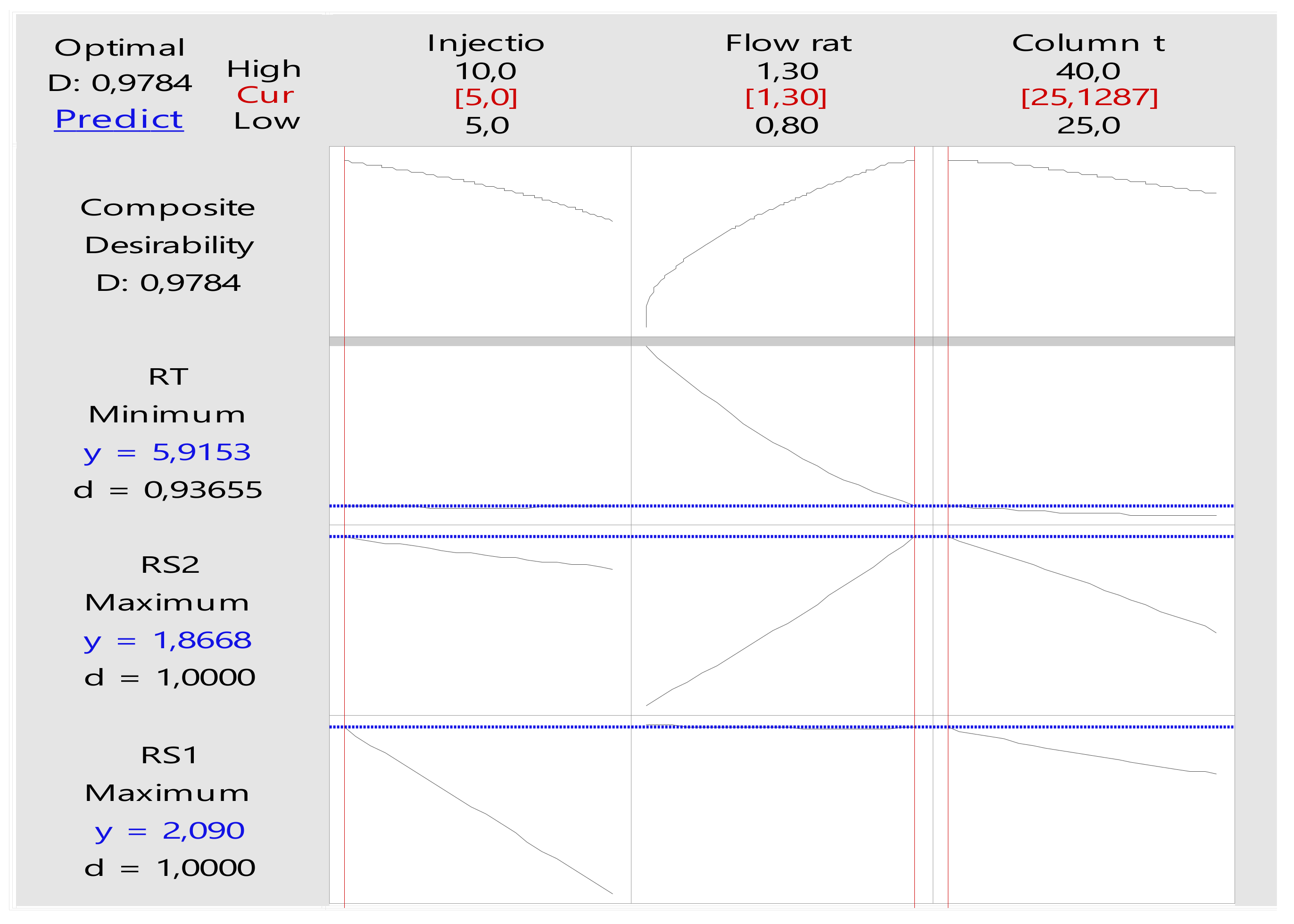
3.2. Optimisation of the HPLC-DAD Method Using Design of Experiment (DoE)

Design of experiment (DoE), unlike one-factor-at-a-time, assesses the significance of the parameters/factors and their interactions on the response. Based on the knowledge gained from optimisation using one-factor-at-a-time, injection volume, flow rate and column temperature were identified as the critical factors. Resolution between C2 and C3 (RS1), resolution between C4 and C5 (RS2), and retention time (t_R) of the last eluting compounds (C7) were identified as the responses. Box–Behnken design and response surface methodology were used to establish the optimum conditions. Analysis of variance (ANOVA) was used to analyse the results at 95% confidence level while the surface plots were utilised to visualise the results. The polynomial equation as given in Section 2.5 was used to construct the regression models for the responses. The Box–Behnken experimental design obtained using Minitab 18 is shown in Table 1. These experiments were conducted and the responses that were obtained are also shown in Table 1.

Table 1. Box–Behnken design results.

Injection Volume	Flow Rate	Temperature	RS1	RS2	tR
5.0	1.3	32.5	1.99	1.65	5.85
7.5	1.3	40	1.56	1.28	5.81
5.0	0.8	32.5	2.00	0.98	7.40
7.5	1.05	32.5	1.66	1.29	6.44
7.5	1.05	32.5	1.55	1.11	6.39
10.0	1.05	40.0	1.17	0.98	6.39
5.0	1.05	40	1.92	1.13	6.39
10.0	0.80	32.5	1.20	0.96	7.40
7.5	0.80	25.0	1.72	1.06	7.47
10.0	1.05	25.0	1.36	1.36	6.51
7.5	0.80	40.0	1.54	0.86	7.33
5.0	1.05	25.0	2.09	1.44	6.51
7.5	1.30	25.0	1.76	1.78	5.91
10.0	1.30	32.5	1.32	1.47	5.85
7.5	1.05	32.5	1.66	1.28	6.45

RS1 is the resolution between C2 and C3; RS2 is the resolution between C4 and C5; t_R is the retention time of C7.

Table 1. Box–Behnken design results.

Injection Volume	Flow Rate	Temperature	RS1	RS2	tR
5.0	1.3	32.5	1.99	1.65	5.85
7.5	1.3	40	1.56	1.28	5.81
5.0	0.8	32.5	2.00	0.98	7.40
7.5	1.05	32.5	1.66	1.29	6.44
7.5	1.05	32.5	1.55	1.11	6.39
10.0	1.05	40.0	1.17	0.98	6.39
5.0	1.05	40	1.92	1.13	6.39
10.0	0.80	32.5	1.20	0.96	7.40
7.5	0.80	25.0	1.72	1.06	7.47
10.0	1.05	25.0	1.36	1.36	6.51
7.5	0.80	40.0	1.54	0.86	7.33
5.0	1.05	25.0	2.09	1.44	6.51
7.5	1.30	25.0	1.76	1.78	5.91
10.0	1.30	32.5	1.32	1.47	5.85
7.5	1.05	32.5	1.66	1.28	6.45

RS1 is the resolution between C2 and C3; RS2 is the resolution between C4 and C5; t_R is the retention time of C7.

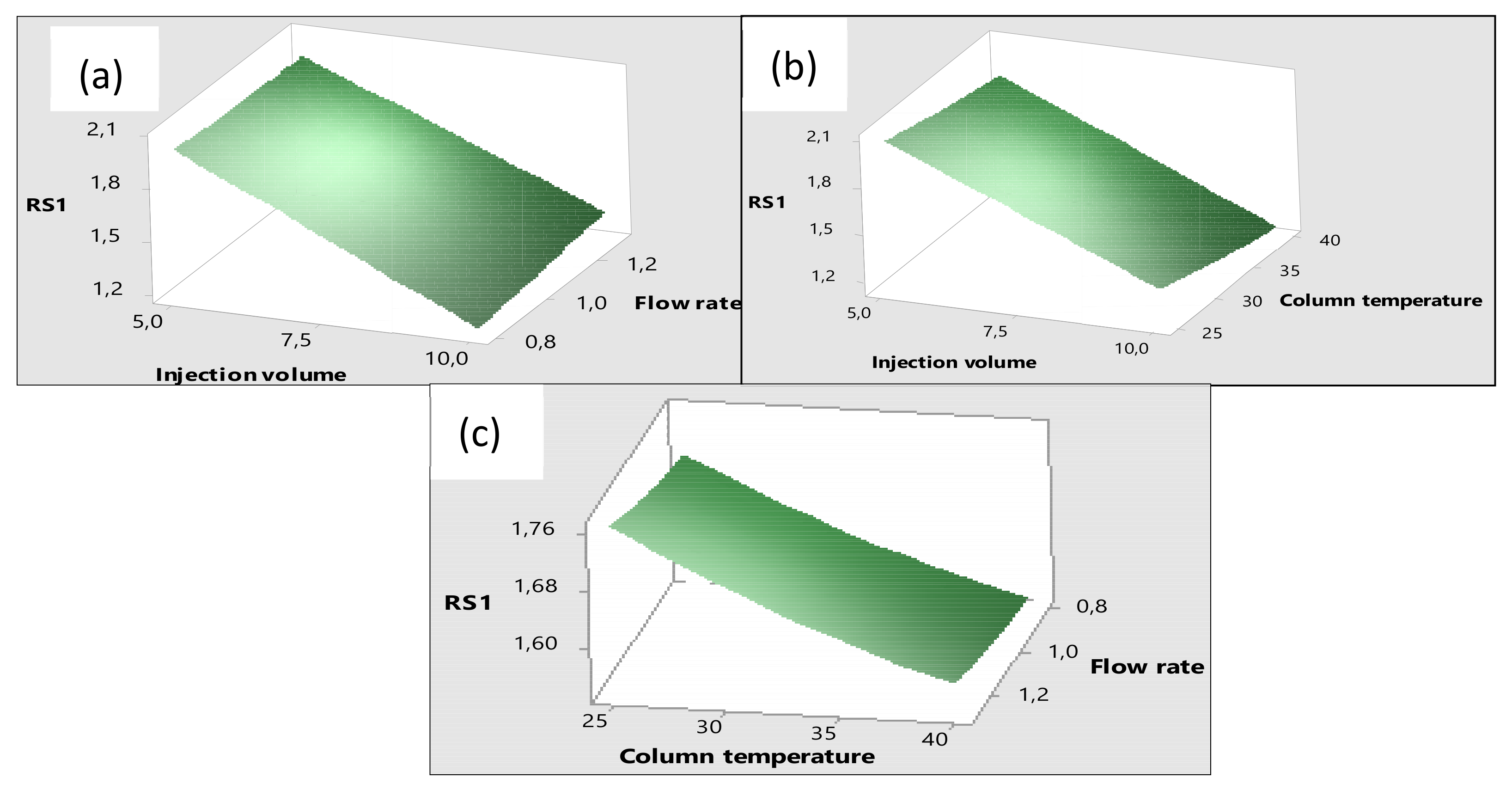
Effects of the Factors on the Responses

The models for the responses were in agreement with the experimental results, as shown by R², R²(adj), and R²(pred) values between 97.9–99.96, 94.13–99.88, and 94.83–99.89, respectively, as shown in

Table 2. ANOVA results for HPLC-DAD method optimisation using Box–Behnken design.

	RS1		RS2		tR
R2	99.28		97.90		99.96
R2(adj)	97.99		94.13		99.88
R2(pred)	97.94		94.83		99.89
	P-value	Coefficient	P-value	Coefficient	P-value	Coefficient
Linear	0.00		0.00		0.00
Second	0.90		0.83		0.00
Interaction	0.51		0.18		0.82
Constant	0.00	1.6233	0.00	1.2267	0.00	6.4267
Injection volume	0.00	−0.3688	0.065	−0.0537	1.00	0.000
Flow rate	0.20	0.0213	0.00	0.2900	0.00	−0.7725
Column temperature	0.00	−0.0925	0.00	−0.1738	0.00	−0.0600
Injection volume2	0.90	−0.0029	0.77	0.0104	0.43	0.0092
Flow rate2	0.75	0.0071	0.44	0.0279	0.00	0.1892
Column temperature2	0.53	0.0146	0.49	−0.0096	0.24	0.0142
Injection volume * flow rate	0.18	0.0325	0.27	−0.0400	1.00	0.0000
Injection volume * column temp	0.82	−0.0050	0.61	−0.0175	1.00	0.0000
Flow rate * column temperature	0.82	−0.0050	0.07	−0.0750	0.38	0.0100
Lack-of-fit	0.99		1.00		1.00

* Meaning interaction between the factors.

. The p-values in Table 2 indicate whether a parameter has a significant or insignificant effect on a response. A p-value of less than 0.05 indicates that the parameter has a significant effect on the response and p-values greater than 0.05 indicate an insignificant effect. The sign of the coefficient indicates the relationship between the parameter and the response where a positive sign indicates a direct relationship and a negative sign indicates an inverse relationship. Linear models for all the responses had p-value of 0.00 meaning that the models were significant. The second order model for t_R was also significant, shown by p = 0.00. The second order models for RS1 and RS2 had p-values of 0.93 and 0.83, respectively, meaning that the models were not significant (Table 2). None of the interaction models were significant, as shown by p-values being greater than 0.05. The lack of fit for all the models was not significant, meaning that the experimental data can be used to predict the responses. Injection volume and column temperature were found to have a significant effect on RS1, shown by p-values of less than 0.05. The coefficient values for these parameters were negative indicating that they had an inverse effect on RS1. The interactions between the factors had an insignificant effect on RS1. Flow rate had a positive significant effect on RS2 while column temperature and the linear interaction between flow rate and column temperature had an inverse significant effect on RS2. Flow rate and column temperature had an inverse significant effect on t_R, while the flow rate also had a quadratic positive significant effect on t_R. Only the significant factors were included in the models for the responses as shown below.

RS1 = 1.6233 − 0.3688x₁ − 0.0925x₃

RS2 = 1.2267 − 0.0537x₁ + 0.2900x₂ − 0.1738x₃

t_R = 6.4267 − 0.7725x₂ − 0.0600x₃ + 0.1892x₂²

where x₁ is injection volume, x₂ is flow rate and x₃ is column temperature.

The effects of the factors on the responses are visualised on the surface plots (Figure 3, Figure 4 and Figure 5). The inverse effect of injection volume and column temperature on RS1 can clearly be observed in Figure 3 whereby an increase in injection volume and column temperature results in a decrease in RS1. Figure 4 shows that an increase in flow rate results in an increase in RS2 while an increase in column temperature results in a decrease in RS2 and injection volume has no observable effect on RS2. Figure 5 also shows that an increase in both flow rate and column temperature results in a decrease in t_R.

The Minitab Response Optimizer was used to identify the experimental conditions that would lead to optimum responses (Figure 6). The Minitab Response Optimizer was set to maximise the resolution (RS1 and RS2) and minimise the retention time (t_R). Injection volume of 5 µL, flow rate of 1.3 mL/min, and column temperature of 25 °C were predicted as the optimum conditions. Desirability functions of 1 were predicted for RS1 and RS2 and 0.94 for t_R. For each response, a desirability function assigns numbers of between 0 and 1, with 0 indicating a response that is completely undesirable, and 1 indicating a response that is completely desirable or ideal, therefore, the closer the desirability function is to 1 the better the response (Figure 6). The predicted conditions were tested experimentally, and the results were used to calculate the experimental desirability functions. The experimental desirability functions were found to be the same as those predicted. Therefore, the predicted conditions were adopted as the optimum conditions. Figure 7 shows the separation of the C1–C7 compounds under the optimum conditions.

3.3. HPLC-DAD Method Validation

The method was validated using the external standard-calibration and standard-addition methods. The standard-addition method was used to minimise the matrix effect that the compounds of interest might encounter in real Mondia whitei samples. The two methods were then compared to assess whether there is any significant difference between them.

3.3.1. Linearity

Linearity results for the methods are shown in

Table 3. Linearity data (regression coefficient), limit of detection ^# and limit of quantification * using the external standard-calibration and standard-addition methods.

Compound Name	Solvent (mg/L)	Root Powder (mg/kg)	Teabag (mg/kg)	Syrup (mg/L)
C1	6.5811x − 0.0106 (0.9995), 0.1 #, 0.5 *	Y = 6.5895x 0.2918 (0.9940), 0.8 #, 2.7 *	Y = 6.5174x + 0.832 (0.9980), 0.6 #, 1.9 *	Y = 6.5183x + 0.7573 (0.9976), 0.6 #, 2.1 *
C2	3.3517x + 0.2585 (0.9959), 0.3 #, 1.0 *	Y = 3.313x + 0.8092 (0.9930), 1.1 #, 3.8 *	Y = 6.5183x + 0.7573 (0.9976), 0.6 #, 2.1 *	Y = 3.1779x + 1.4611 (0.9949), 0.9 #, 3.0 *
C3	Y = 6.7035x + 0.3257 (0.9962), 0.5 #, 1.8 *	Y = 6.827x − 0.3864 (0.9956), 0.9 #, 3.0 *	Y = 6.7576x − 0.4369 (0.9965), 0.8 #, 2.5 *	Y = 6.7626x − 0.265 (0.9950), 0.9 #, 3.0 *
C4	2.1177x + 0.299 (0.9980), 0.5 #, 1.7 *	Y = 2.1324x 0.4067 (0.9949), 1.0 #, 3.4 *	Y = 2.1196x + 0.1178 (0.9926), 1.1 #, 3.7 *	Y = 2.1167x − 0.1433 (0.9915), 1.2 #, 3.9 *
C5	Y = 3.8625x − 0.348 (0.9942), 0.7 #, 2.2 *	Y = 3.8673 − 0.0456 (0.9943), 0.9 #, 3.1 *	Y = 3.8354x + 0.0541 (0.9907), 1.2 #, 4.1 *	Y = 3.7524x + 0.451 (0.9936), 1.0 #, 3.4 *
C6	Y = 3.5614x − 0.2993 (0.9960), 0.9 #, 3.0 *	Y = 3.5878 − 0.3009 (0.9949), 0.9 #, 3.1 *	Y = 3.5938x − 0.7325 (0.9931), 1.1 #, 3.5 *	Y = 3.489x + 0.1656 (0.9926), 1.1 #, 3.7 *
C7	Y = 30.135x − 1.0792 (0.9993), 0.4 #, 1.3 *	Y = 30.115x − 0.6412 (0.9993), 0.4 #, 1.4 *	Y = 30.168x − 1.5828 (0.9986), 0.5 #, 1.6 *	Y = 30.2x − 1.9401 (0.9987), 0.5 #, 1.5 *

^# Indicates the limit of detection values, * indicate the limit of quantification values.

. Both methods were linear as shown by regression coefficients that ranged from 0.9939–0.9995 and 0.9907–0.993 for the external standard-calibration and standard-addition methods, respectively. The regression equations were derived using the least square method.

3.3.2. Limit of Detection and Limit of Quantification

The limit of detection (LOD) values for the external calibration method ranged from 0.1–0.9 mg/L and the limit of quantification (LOQ) values ranged from 0.5–3.0 mg/L. In the root powder, the LOD values ranged from 0.4–1.1 mg/kg, in the teabag they ranged from 0.5–1.2 mg/kg, while in the syrup they ranged 0.5–1.2 mg/L. The lowest LOD of 0.1 mg/L was observed for C1 in the solvent. The LOQ values ranged from 1.4–3.8 mg/kg, 1.6–4.1 mg/kg, and 1.5–3.9 mg/L in the root powder, teabag, and syrup, respectively (Table 3). The highest LOQ was observed for C5 in the teabag sample.

3.3.3. Precision

The precision of the methods was evaluated at three concentration levels, namely the lowest, middle, and highest concentration levels. For the external standard-calibration method, the concentration levels were 1, 7, and 14 mg/L while for the standard-addition method the concentration levels were 3, 9, and 14 mg/kg for solid samples and 3, 9, and 14 mg/L for the syrup. Repeatability of the methods was determined by assessing the intra-day variability of the methods. The percentage relative standard deviation (%RSD) for the external standard-calibration method ranged from 0.3 to 1.7 across the concentration levels (

Table 4. Percentage recoveries, intra-day+ and inter-day * precision (%RSD), and measurement uncertainty (expressed as U (%)) data for the compounds in solvent and the different matrices.

Concentration	C1	C2	C3	C4	C5	C6	C7
Solvent
1 mg/L	1.6+ 3.8 *	1.5+ 4.5 *	1.1+ 1.7 *	1.2+ 4.5 *	1.4+ 3.8 *	1.6+ 3.8 *	1.7+ 4.8 *
7 mg/L	0.6+ 2.2 *	1.2+ 1.1 *	0.8+ 0.5 *	1.2+ 3.8 *	0.8+ 3.0 *	1.2+ 2.9 *	1.6+ 0.6 *
14 mg/L	0.3+ 2.8 *	0.4+ 1.1 *	1.0+ 0.3 *	0.6+ 3.6 *	0.4+ 2.4 *	0.3+ 3.4 *	0.7+ 0.5 *
Root powder
3 mg/kg	66.1 6.9+ 8.6 *	82.9 6.5+ 11.7 *	94.5 7.3+ 9.8 *	96.7 6.4+ 8.2 *	97.9 5.5+ 6.9 *	89.8 5.0+ 4.2 *	92.4 4.1+ 3.6 *
9 mg/kg	92.8 3.7+ 4.2 *	94.5 4.2+ 6.8 *	96.2 3.2+ 4.4 *	99.3 3.9+ 5.4 *	100.5 2.6+ 2.9 *	94.6 3.4+ 3.6	99.6 1.4+ 4.4
14 mg/kg	101.6 1.3+ 3.6 *	98.0 4.8+ 4.0 *	99.5 2.9+ 3.9 *	101.5 3.4+ 3.2 *	103.2 2.8+ 2.3 *	99.7 3.2+ 2.5 *	103.5 1.3+ 2.3 *
U (%)	24.1	19.0	16.0	14.6	5.9	5.8	6.3
Teabag
3 mg/kg	89.9 3.9+ 5.1 *	74.5 4.5+ 6.8 *	90.0 3.9+ 4.7 *	80.2 6.0+ 9.4 *	90.2 4.8+ 9.3	74.4 4.8+ 8.2 *	94.5 5.5+ 4.3 *
9 mg/kg	90.2 2.6+ 1.7 *	94.3 2.3+ 4.9 *	94.8 2.9+ 3.1 *	99.4 2.3+ 2.3 *	96.4 3.0+ 3.9 *	89.8 3.0+ 4.0 *	98.3 1.8+ 4.9 *
14 mg/kg	99.4 1.3+ 2.4 *	105.6 1.3+ 1.5 *	98.7 2.1+ 3.6 *	101.5 4.7+ 2.6 *	99.1 2.4+ 3.6 *	95.7 1.8+ 2.1 *	102.4 1.4+ 2.2 *
U (%)	10.1	17.8	10.6	19.1	12.1	18.2	11.9
Syrup
3 mg/L	77.6 2.8+ 5.7 *	80.1 3.9+ 7.9 *	94.3 3.2+ 4.3 *	90.4 5.0+ 6.4 *	89.8 5.3+ 6.3 *	90.4 3.1+ 7.0 *	95.6 2.7+ 3.3 *
9 mg/L	89.9 3.0+ 4.9 *	88.3 5.0+ 2.5 *	95.0 1.9+ 3.0 *	96.7 2.4+ 3.0 *	93.4 31.6+ 2.0 *	92.0 1.7+ 1.8 *	98.4 1.1+ 1.9 *
14 mg/L	92.3 2.4+ 1.7 *	96.7 2.6+ 1.2 *	101.6 2.4+ 1.1 *	98.3 2.1+ 2.9 *	100.8 1.7+ 1.1 *	98.6 1.4+ 1.5 *	105.7 0.4+ 0.8 *
U (%)	15.5	15.0	8.7	12.2	12.6	8.8	6.92

+ Indicates the intra-day variability values and * indicates the inter-day variability values.

). The %RSD values that are less than 2% for the external standard-calibration method indicate that the method is repeatable. The %RSD values across all the concentration levels ranged from 1.3–7.3, 1.3–6.0, and 0.4–5.3 for the root powder, teabag, and syrup, respectively. The %RSD values that are less than 10% in the matrix for intra-day variability show that the method is repeatable (Table 4).

Inter-day (intermediate) variability using the external standard-calibration method and the standard-addition method was assessed over five consecutive days. The %RSD values for the external standard-calibration method ranged from 0.3–4.8, with C7 having the highest %RSD value (4.8) at the lowest concentration level (1 mg/L). For the root powder, teabag, and syrup matrices, the %RSD values ranged from 2.3–11.7 and 1.5–9.4 and 0.8–7.9, respectively, with C2 having the highest %RSD in both the root powder and syrup matrices and compound C4 in the teabag. The lowest %RSD value of 0.8 (inter-day variability) was observed for C7 in the syrup matrix at the highest concentration level (Table 4).

3.3.4. Accuracy and Recovery

The accuracy of the method was evaluated by determining the recovery of the method where percentage recovery was calculated using Equation (4) and the results are shown in Table 4. The compounds were extracted from the root powder and teabag using the method described in Section 2.4. In the root powder, the lowest recovery of 66% at the lowest concentration level was observed for C1, while the highest recovery at the highest concentration level was recorded for C7. Overall, the percentage recovery in the root powder ranged from 66.1–97.9%, 92.8–100.5%, and 98.0–103.5% at the lowest, middle, and highest concentration levels, respectively. The percentage recoveries in the teabag matrix ranged from 74.4–94.5%, 89.8–99.4%, and 95.7–105.6% at the lowest, middle, and highest concentration levels, respectively. Overall, the lowest recovery at the lowest concentration level in the teabag matrix was observed for C6, while the highest recovery at the highest concentration level was recorded for C2. In the syrup, the percentage recoveries ranged from 77.6–95.6% at the lowest concentration level, 88.3–98.4% at the middle concentration level, and 92.3–105.7% at the highest concentration level. Overall, the lowest recovery in the syrup was observed for C2 and the highest for C3.

3.3.5. Measurement Uncertainty

The top-down approach was used to assess the measurement uncertainty (U) of the method. The measurement was based on uncertainty due to precision and recovery. The measurement uncertainty was determined at 95% confidence level using Equations (5)–(7) given in Section 2.6.6 and the results are listed in Table 4. The measurement uncertainty in the root powder matrix ranged from 5.8–24.1 with C1 having the highest measurement uncertainty. This is due to the low recovery of this compound at the lowest concentration level. In the teabag matrix, the measurement uncertainty ranged from 10.1–19.1, with the lowest measurement uncertainty observed for C1 and the highest for C4. Measurement uncertainty in the syrup matrix ranged from 6.9–15.5, with C1 exhibiting the lowest measurement uncertainty, and C7 the highest. Measurement uncertainty for the compounds can be improved by using the bottom-up approach instead of the top-down approach, whereby all the sources of error can be determined and reduced.

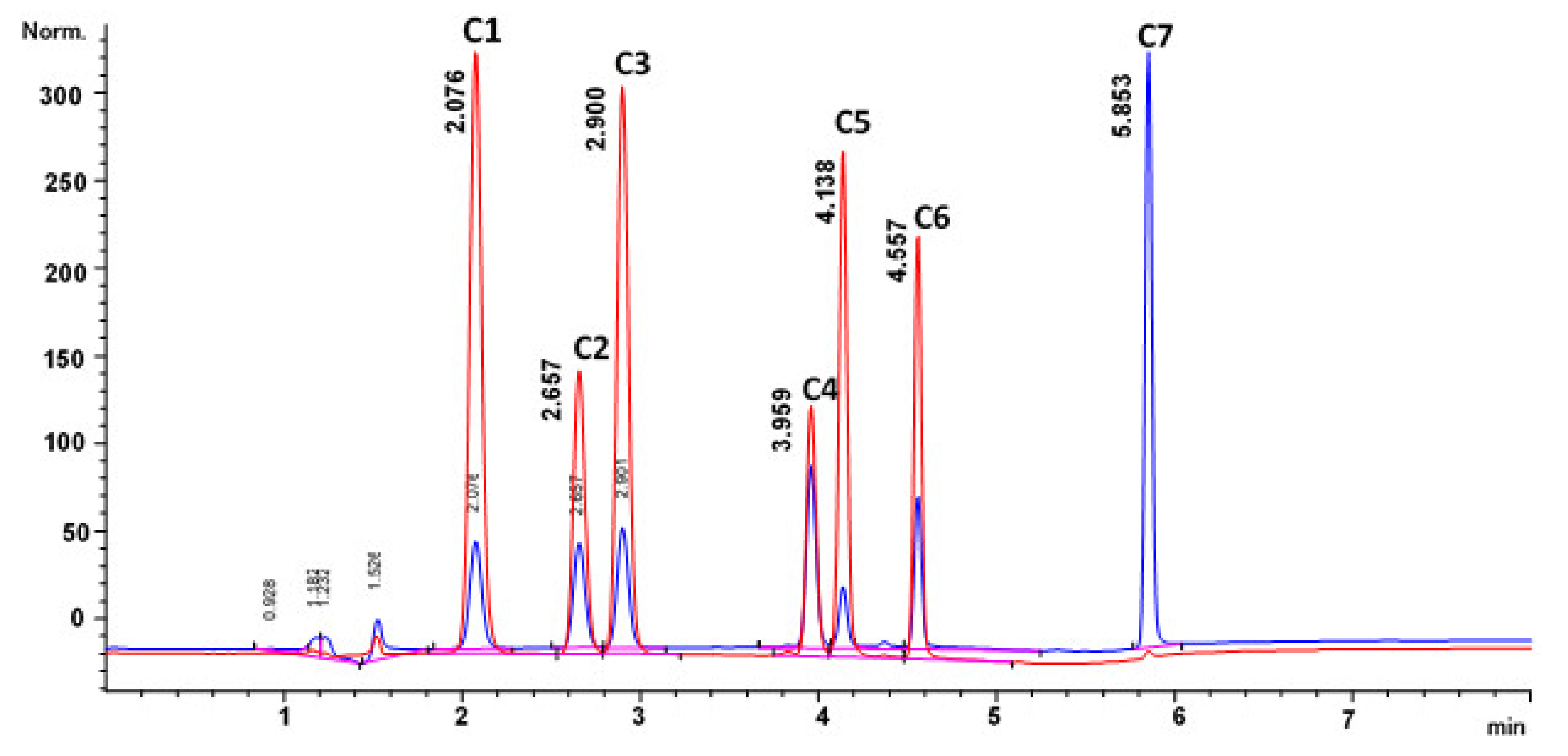
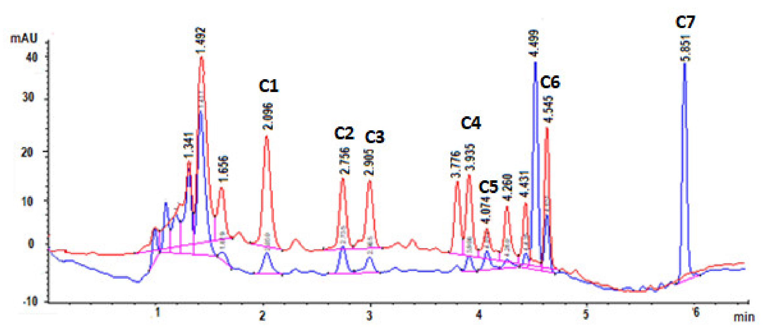
3.3.6. Specificity of the Method

The specificity of the method was assessed by comparing the peaks that represent the compounds of interest in the pure solvent and in the different matrices. The retention times of peaks that represented the compounds of interest in the matrices were compared with those in the pure solvent and the standard deviation of the results was between 0.06–0.09. The percentage purity of the peaks in the different matrices was between 0.95–0.99. These results indicated that the method is specific for the compounds of interest.

3.4. Comparison of the External Standard-Calibration and Standard-Addition Methods

The Minitab software was used to assess any significant difference between the two methods by using the t-test and p-value at a 95% confidence level. The critical t-value with 12 degrees of freedom is 1.782.

Table 5. The t- and p-values for comparing the difference between the external standard-calibration and standard-addition methods.

External Standard-Calibration Method vs. the Standard-Addition Method
	Root Powder	Teabag	Syrup
t-value	−0.00	−0.00	0.01
p-value	0.997	0.932	0.994

shows the t-values for the different matrices which were all less than the t-critical value. The p-values for the different matrices were all greater than 0.05. These results indicate that there is no statistical difference between the two methods. Therefore, any of these methods can be used to quantify the compounds of interest in real Mondia whitei samples.

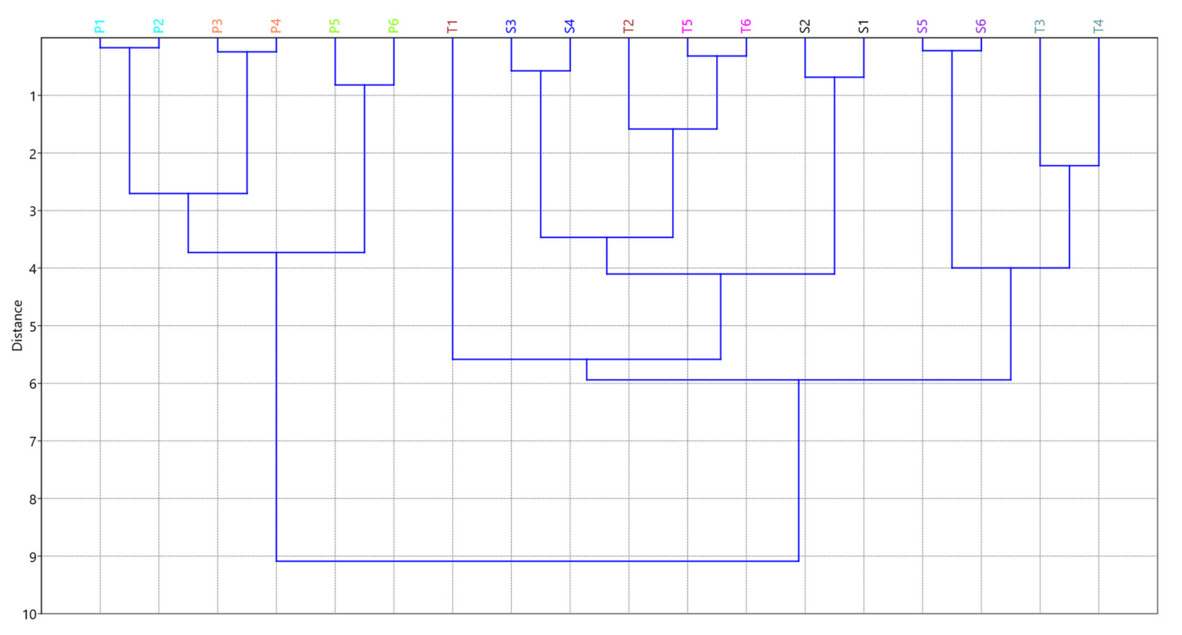
3.5. Quantification of the Compounds of Interest in Real Mondia whitei Samples

Extraction from real Mondia whitei samples was carried out using the extraction method described in Section 2.4. The extracts were separated using the developed and validated method. Quantification of the compounds of interest was carried out using the standard-addition method regression equations. Figure 8 shows a chromatogram representing the separation of the root sample P1. Chromatograms for the separation of one sample each from the teabag and syrup samples are given in the Supplementary Materials (Figures S1 and S2). The compounds C2, C3, C4, and C6 were detected in all the samples with C3 and C4 being detected in some samples at concentrations below the limit of quantification (

Table 6. Quantitative analysis results for the different Mondia whitei samples (compound concentration in solid samples (mg/kg) and in syrup samples (mg/L)).

	REGION	C1	C2	C3	C4	C5	C6	C7
S1	M1	<LOD	8.5	6.5	4.5	<LOD	10.6	<LOD
S2	M1	<LOD	8.3	6.8	4.0	<LOD	10.3	<LOD
S3	M2	2.4	8.6	4.4	6.1	<LOD	9.5	<LOD
S4	M2	2.6	8.4	4.1	6.1	<LOD	9.9	<LOD
S5	M3	<LOD	8.7	<LOQ	7.0	<LOQ	9.6	<LOD
S6	M3	<LOD	8.6	<LOQ	7.0	<LOQ	9.4	<LOD
T1	M4	<LOQ	5.9	5.6	<LOQ	<LOQ	10.6	<LOD
T2	M4	2.4	5.7	5.6	3.8	<LOQ	10.6	<LOD
T3	M5	2.7	7.2	2.3	5.0	<LOD	9.8	<LOD
T4	M5	2.7	7.4	<LOQ	4.8	<LOD	9.7	<LOD
T5	M6	3.3	6.1	5.0	4.1	<LOD	9.6	<LOD
T6	M6	3.2	6.4	5.0	4.1	<LOD	9.6	<LOD
P1	KZN	3.0	9.6	6.0	6.9	<LOQ	11.8	5.6
P2	KZN	3.1	9.6	6.1	6.8	<LOQ	11.8	5.6
P3	KZN	4.4	9.4	6.9	7.2	<LOQ	9.7	6.0
P4	KZN	4.5	9.4	6.9	7.2	<LOQ	9.8	6.2
P5	KZN	5.0	10.9	7.1	9.7	<LOQ	11.5	6.9
P6	KZN	5.1	10.9	7.1	9.6	<LOQ	11.6	6.1

). The C7 compound was detected only in the root samples. The root samples contained very high amounts of C6 as compared to the other samples. This compound is reported to have antibacterial activity and is responsible for the odour of the plant [18,19,20]. Studies show that compounds such as C3 and C6 display positive biological activities at concentrations from 50–100 mg/kg [18,20]. Therefore, it is recommended that the products such as teabag and syrup should contain these compounds at concentrations between 50 and 100 mg/kg.

Principle component analysis was used to examine the variability between the different samples. The PCA-biplot (Figure 9) and hierarchical clustering plot (Figure 10) show the variance and correlation between the samples. On the PCA-biplot, PC1 describes 70.33% of the variance in the data while PC2 describes 20.51%. The variance between the root samples and the other samples is shown by their separation along PC1 on the PCA-biplot. This is also observed on the hierarchical cluster plot where the roots are correlated to the other samples at a higher level. Both plots show that, for the most part, samples from the same manufacturer are closely correlated. However, this is not the case for teabag samples T1 and T2. The difference between these samples is observed on both the PCA-biplot where they are not clustered together, and on the hierarchical clustering plot which shows that T2 is closely correlated to T5 and T6, and not to T1. Both plots also show that products that are the same but produced by different manufacturers are different. For example, syrup samples S5 and S6 were shown to be more closely correlated to teabag samples T3 and T4 than they are to other syrup samples, and the same is true for the teabag samples. The difference between the syrup samples S1 and S2 and the other syrup samples is shown by their separation along PC2. These results show the need for quality control of these products.

4. Conclusions

A simple, fast and easy HPLC-DAD method for the simultaneous separation and determination of seven compounds found in Mondia whitei was developed and validated. The method was used successfully to quantify the compounds of interest in Mondia whitei products found in the market and root samples from different areas in the KwaZulu-Natal Province of South Africa. The compounds: 3-hydroxy-4-methoxy benzaldehyde (C2), 7-hydroxy-6-methoxy coumarin (C3), coumarin (C4), and 2-hydroxy-4-methoxy benzaldehyde (C6) were detected in all the products and samples that were analysed. The samples and products were found to contain high amounts of 2-hydroxy-4-methoxy benzaldehyde (C6) as compared to the other compounds. However, the concentration of 2-hydroxy-4-methoxy benzaldehyde that was detected in the products is still lower than 100 mg/kg. This is the concentration where positive biological activities for this compound is achieved according to reports. Therefore, it is recommended that the products should contain the compounds of interest with concentrations between 50 and 100 mg/kg. The current calibration range for the method is from 3–14 mg/kg, this was chosen because the compounds are found in the products within this range. However, the calibration range can be extended to enable quantification of the compounds up to 100 mg/kg.

References

1. Mbamalu, O.N.; Antunes, E.; Silosini, N.; Samsodien, H.; Syce, J. HPLC determination of selected flavonoid glycosides and their corresponding aglycones in Sutherlandia frutescens materials. Med. Aromat. Plants 2016, 5, 1–10. [Google Scholar] [CrossRef] [Green Version]
2. Bharathi, A.; Yan-Hong, W.; Smillie, T.J.; Fu, X.; Li, X.C.; Mabusela, W.; Syce, J.; Johnson, Q.; Folk, W.; Khan, I.A. Quantitative determination of flavonoids and cycloartanol glycosides from aerial parts of Sutherlandia frutescens (L.) R. BR. by using LC-UV/ELSD methods and confirmation by using LC-MS method. J. Pharm. Biomed. Anal. 2010, 52, 173–180. [Google Scholar] [CrossRef] [Green Version]
3. Engsuwan, J.; Waranuch, N.; Limpeanchob, N.; Ingkaninan, K. HPLC methods for quality control of Moringa oleifera extract using isothiocyanates and astragalin as bioactive markers. ScienceAsia 2017, 34, 169–174. [Google Scholar] [CrossRef] [Green Version]
4. Chokwe, R.C.; Dube, S.; Nindi, M.M. Development of an HPLC-DAD method for the quantification of ten compounds from Moringa oleifera Lam. and its application in quality control of commercial products. Molecules 2020, 25, 4451. [Google Scholar] [CrossRef] [PubMed]
5. Aremu, A.O.; Cheesman, L.; Finnie, J.F.; Van Staden, J. Mondia whitei (Apocynaceae): A review of its biological activities, conservation strategies and economic potential. S. Afr. J. Bot. 2011, 77, 960–971. [Google Scholar] [CrossRef] [Green Version]
6. Stafford, G.I.; Pedersen, M.E.; Van Staden, J.; Jäger, A.K. Review on plants with CNS-effects used in traditional South African medicine against mental diseases. J. Ethnopharmacol. 2008, 119, 513–537. [Google Scholar] [CrossRef] [PubMed]
7. Odugbemi, T.O.; Akinsulire, O.R.; Aibinu, I.E.; Fabeku, P.O. Medicinal plants useful for malaria therapy in Okeigbo, Ondo State, Southwest Nigeria. Afr. J. Tradit. Complement. Altern. Med. 2007, 4, 191–198. [Google Scholar] [CrossRef] [PubMed] [Green Version]
8. Sewani-Rusike, C.R.; Iputo, J.E.; Ndebia, E.J.; Gondwe, M.; Kamadyaapa, D.R. A comparative study on the aphrodisiac activity of food plants Mondia whitei, Chenopodium album, Cucurbita pepo and Sclerocarya birrea extracts in male wistar rats. Afr. J. Tradit. Complement. Altern. Med. 2015, 12, 22–26. [Google Scholar] [CrossRef] [Green Version]
9. Watcho, P.; Zelefack, F.; Ngouela, S.; Nguelefack, T.B.; Kamtchouing, P.; Tsamo, E. Enhancement of erectile function of sexually naïve rats by β -sitosterol and α- β -amyrin acetate isolated from the hexane extract of Mondia whitei. Asian Pac. J. Trop. Biomed. 2012, 2, S1266–S1269. [Google Scholar] [CrossRef]
10. Watcho, P.; Donfack, M.M.; Zelefack, F.; Nguelefack, T.B.; Wansi, S.; Ngoula, F.; Kamtchouing, P.; Tsamo, E.; Kamanyi, A. Effects of the hexane extract of Mondia whitei on the reproductive organs of male rats. Afr. J. Tradit. Complementary Altern. Med. 2005, 2, 302–311. [Google Scholar] [CrossRef] [Green Version]
11. Martey, O.N.K.; He, X. Possible mode of action of Mondia whitei: An aphrodisiac used in the management of erectile dysfunction. J. Pharmacol. Toxicol. 2010, 5, 460–468. [Google Scholar] [CrossRef] [Green Version]
12. Quasie, O.; Martey, O.N.K.; Nyarko, A.K.; Gbewonyo, W.S.K.; Okine, L.K.N. Modulation of penile erection in rabbits by Mondia whitei: Possible mechanism of action. Afr. J. Tradit. Complementary Altern. Med. 2010, 7, 241–252. [Google Scholar] [CrossRef] [PubMed] [Green Version]
13. Lampiao, F. The role of Mondia whitei in reproduction: A review of current evidence. Internet J. Third World Med. 2008, 8, 1–3. [Google Scholar]
14. Patnam, R.; Kadali, S.S.; Koumaglo, K.H.; Roy, R. A chlorinated coumarinolignan from the African medicinal plant. Mondia Whitei. Phytochem. 2005, 66, 683–686. [Google Scholar] [CrossRef]
15. Mukonyi, K.W.; Ndiege, I.O. 2-hydroxy-4-methoxybenzaldehyde: Aromatic taste modifying compound from Mondia whytei skeels. Bull. Chem. Soc. Ethiop. 2001, 15, 137–141. [Google Scholar]
16. Kundu, A.; Mitra, A. Methoxybenzaldehydes in plants: Insight to the natural resources, isolation, application and biosynthesis. Curr. Sci. 2016, 111, 1325–1334. [Google Scholar] [CrossRef]
17. Wang, J.; Liu, H.; Zhao, J.; Gao, H.; Zhou, L.; Liu, Z.; Chen, Y.; Sui, P. Antimicrobial and antioxidant activities of the root bark essential oil of Periploca sepium and its main component 2-hydroxy-4-methoxybenzaldehyde. Molecules 2010, 15, 5807–5817. [Google Scholar] [CrossRef] [PubMed] [Green Version]
18. Harohally, N.V.; Cherita, C.; Bhatt, P.; Anu Appaiah, K.A. Antiaflatoxigenic and antimicrobial activities of Schiff bases of 2-hydroxy-4-methoxybenzaldehyde, cinnamaldehyde, and similar aldehydes. J. Agric. Food Chem. 2017, 65, 8773–8778. [Google Scholar] [CrossRef]
19. Xu, L.; Zhao, X.-Y.; Wu, Y.-L.; Zhang, W. The study on biological and pharmacological activity of coumarins. In Proceedings of the Asia-Pacific Energy Equipment Engineering Research Conference, Zhuhai, China, 13–14 June 2015; Volume 9, pp. 135–138. [Google Scholar] [CrossRef] [Green Version]
20. Bhattacharyya, S.S.; Paul, S.; Dutta, S.; Boujedaini, N.; Khuda-Bukhsh, A.R. Anti-oncogenic potentials of a plant coumarin (7-hydroxy-6-methoxy coumarin) against 7,12-dimethylbenz[a]anthracene-induced skin papilloma in mice: The possible role of several key sihnal proteins. J. Chin. Integr. Med. 2010, 7, 645–654. [Google Scholar] [CrossRef]
Figure 1. The structures of the compounds of interest in the study.
Processes 09 01864 g001aProcesses 09 01864 g001b
Figure 2. Separation of the C1‒C7 using a gradient elution mode commencing at 0 min 25% B, 2 min 40% B, 3 min 65% B, 4 min 100% B, with a run time of 6.5 min. Injection volume of 5 µL, flow rate of 1 mL min−1, and temperature of 25 °C, at λ = 254 nm (blue) and λ = 331.4 nm (red).
Processes 09 01864 g002
Figure 3. (a) The surface plot of the effects of injection volume and flow rate on RS1 while keeping temperature constant; (b) effects of injection volume and column temperature on RS1 while keeping flow rate constant; and (c) effects of column temperature and flow rate on RS1 while keeping injection volume constant.
Processes 09 01864 g003
Figure 4. (a) The surface plot of the effects of injection volume and column temperature on RS2 while keeping flow rate constant; (b) effects of injection volume and flow rate on RS2 while keeping column temperature constant; and (c) effects of column temperature and flow rate on RS2 while keeping injection volume constant.
Processes 09 01864 g004
Figure 5. (a) The surface plot of the effects of flow rate and column temperature on tR while keeping injection volume constant; (b) effects of injection volume and flow rate on tR while keeping column temperature constant; and (c) effects of column temperature and injection volume on tR while keeping flow rate constant.
Processes 09 01864 g005
Figure 6. The predicted HPLC-DAD separation conditions using Minitab Response Optimizer.
Processes 09 01864 g006
Figure 7. Separation of the C1–C7 under optimised conditions using a gradient elution mode commencing at 0 min 25% B, 2 min 40% B, 3 min 65% B, 4 min 100% B with a run time of 6.5 min. Injection volume of 5 µL, flow rate of 1.3 mL/min, and temperature of 25 °C, at λ = 254 nm (blue) and λ = 331.4 nm (red).
Processes 09 01864 g007
Figure 8. A chromatogram representing the separation of root sample P1 using the validated method.
Processes 09 01864 g008
Figure 9. PCA biplot showing the variance between the M. whitei products.
Processes 09 01864 g009
Figure 10. Hierarchical clustering plot showing the correlation between the different M. whitei product samples.
Processes 09 01864 g010