Multiresolution Forecasting for Industrial Applications

Abstract

The forecasting of univariate time series poses challenges in industrial applications if the seasonality varies. Typically, a non-varying seasonality of a time series is treated with a model based on Fourier theory or the aggregation of forecasts from multiple resolution levels. If the seasonality changes with time, various wavelet approaches for univariate forecasting are proposed with promising potential but without accessible software or a systematic evaluation of different wavelet models compared to state-of-the-art methods. In contrast, the advantage of the specific multiresolution forecasting proposed here is the convenience of a swiftly accessible implementation in R and Python combined with coefficient selection through evolutionary optimization which is evaluated in four different applications: scheduling of a call center, planning electricity demand, and predicting stocks and prices. The systematic benchmarking is based on out-of-sample forecasts resulting from multiple cross-validations with the error measure MASE and SMAPE for which the error distribution of each method and dataset is estimated and visualized with the mirrored density plot. The multiresolution forecasting performs equal to or better than twelve comparable state-of-the-art methods but does not require users to set parameters contrary to prior wavelet forecasting frameworks. This makes the method suitable for industrial applications.

1. Introduction

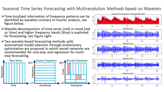
Seasonal time series forecasting with computers had early success with seasonal adjusted methods as proposed in 1978 [1] or with the the X-11 method [2]. Over the years, improved versions, such as the X-13 [3], various variants of such models and new techniques in the area of statistical models, were developed [4], and a new field emerged in computational intelligence dealing with seasonal time series forecasting arose [5]. Recently, a method based on Fourier analysis was introduced [6]. Fourier analysis can be used for estimating seasonal components in a time series. The frequency content of a time series over its complete range can be approximated with Fourier analysis. Varying seasonality imposes a problem for forecasting methods that assume a non-varying seasonality, because Fourier analysis gives only a representation of the frequency content of a time series and does not give a relation of frequency patterns to specific time intervals [7]. For example, the relationship of high frequency peaks at a specific time interval cannot be captured by Fourier analysis [7]. Different frequencies can be captured with Fourier analysis as part of the whole time series without a specific relation to time intervals. The recognition of high frequencies is constrained by the sample rate (Nyquist–Shannon sampling theorem [8]), whereas for low frequencies, it is constrained by the total length of the time series itself.

In contrast, the wavelet analysis uses short time intervals for capturing high frequencies in order to relate them to specific time intervals (localization in time) more precisely than Fourier analysis. Low frequencies are treated with longer time intervals (compared to the high frequencies), since the recognition of low frequencies depends on the maximal length of the time interval used for analysis. Large high frequency bands are captured with small time intervals, whereas the small low frequency bands are captured with large time intervals. Therefore, it is interesting to apply wavelet analysis for seasonal time series forecasting in order to investigate the potential of such a model to adapt to complex seasonal structures. In this work, two time series forecasting methods using the redundant Haar wavelet decomposition were implemented and compared to several state-of-the-art forecasting methods, including a Fourier method [6] and other multiresolution methods [9,10]. The rough sketch of the wavelet algorithm is based on [11,12,13,14,15], but no software was referenced there. Moreover, no method for efficiently computing the best coefficient selection from their prediction scheme existed.

Thus, we propose the use of a differential evolutionary optimization strategy to solve the complex model selection problem in the wavelet forecasting concept introduced by [16]. This strategy does not require the user to set any parameters since such a task can be performed automatically by computational intelligence. The two algorithms are open-source and provided in Python and R [17,18] without the necessity to manually set parameters.

Currently, the following methods in Python or R for computing the wavelet decomposition for different task and with different approaches are accessible: signal processing with the continuous wavelet transform [19], signal and image processing with various wavelet transforms [20,21], wavelet analysis with scalogram tools [22], univariate and bivariate wavelet analysis [23], wavelet analysis (Angi, R.; Harald, S., 2018), signal processing [24], signal processing for one to three dimensions [25], wavelet statistics [26] and testing white noise with wavelets [27]. There are three packages in R dealing with time series forecasting with the wavelet decomposition, but all three packages require the user to set parameters. The first uses a redundant Haar wavelet decomposition in combination with an ARIMA framework [28,29]. The second one uses a redundant Haar wavelet decomposition combined with an artificial neural network [30,31]. The last one uses GARCH and is of no interest here [32].

There has been a plethora of developments in time series forecasting over the last four decades [4]. The main direction is to evaluate forecasting techniques on out-of-sample forecasts [33], perform model selection with a cross validation [34] and to compare results with relative or scaled errors [35]. Much effort was put in empirical studies [36,37,38,39], comparing many techniques across multiple datasets, which was recommended for classification tasks by [40]. The naïve method forecasts the time series by continuing the last value. Adapted to seasonality patterns, the last value of the last season of the forecast is taken. In this work, such a method will be defined as seasonal naïve. The assumption is that any forecasting method should at least outperform the seasonal naïve method [36,37,38,39].

The main contribution of this work is as follows:

• An open-source and application-oriented wavelet framework combined with an automatic model selection through differential evolutionary optimization with standardized access in Python and R.
• Contrary to prior works, a systematic comparison of state-of-the-art methods and open-source accessible seasonal univariate forecasting methods to our framework.
• Wavelet forecasting performs equally well on short-term and long-term forecasting.

This work is structured as follows. Section 2 explains the forecasting setting and presents the multiresolution forecasting method for which the software is available on pypi and CRAN [17,18]. The cross validation designed for time series forecasting is outlined, datasets are introduced, the quality measures are defined and justified, and an estimation and visualization technique for the distribution is presented. Section 3 shows the results with a scaled quality measure used for benchmarking. The results with a relative error are in Appendix B. Section 4 discusses the results and Section 5 closes with a conclusion.

2. Materials and Methods

The first Section 2.1 outlines the selection of open-source available time series forecasting algorithms. Section 2.2 explains an adaptation of cross validation for out-of-sample forecasts, which is used for the computations and whose results are presented in Section 3. Section 2.3 illustrates the datasets which are used for evaluation and outlines their industrial application. Section 2.4 and Section 2.5 define the quality measures used here to evaluate the forecast errors computed with Section 2.2. Section 2.6 presents an estimation and visualization technique for probability density functions, which is used to analyze the samples obtained with the two quality measures from Section 2.4 and Section 2.5. The last Section 2.7 presents the multiresolution method.

2.1. Related Work

The focus of this work is the forecasting of seasonal univariate time series. Therefore, open access forecasting methods are selected that are specially designed for dealing with seasonality (periodic patterns) independently of the classification into short- and long-term methods. Although in the general case different forecast horizons require different methods [41], Fourier decomposition of time series allows to use methods, such as Prophet, in both cases [6]. Moreover, short- and long-term forecasting strategies usually depend strongly on the resolution of the time series [42,43], whereas periodic patterns do not necessarily depend on the resolution. Hence, the performance of all methods over all 14 horizons are computed and grouped by horizon one versus horizon above one (multi-step). Implicitly, the performance of the one-step forecasts represents a short-term evaluation, and the multi-step forecasts represent a long-term evaluation. In both cases, the distribution is estimated visualized separately with the MD plot [44]. The performance of the method is evaluated with rolling forecasting origins [34] on multiple datasets competing against 10 other forecasting techniques. To the knowledge of the authors, no systematic benchmarking using wavelet forecasting was performed so far. The 12 forecasting techniques were selected, according to their potential of dealing with seasonal time series and their open-source accessibility.

As it is a common issue in data science that published techniques are not implemented (e.g., swarm-based techniques [45]), this work focuses on methods for which open-source implementations are provided through either the Comprehensive R Archive Network (CRAN) or the Python Package Index (pypi). The current state-of-the-art method, according to accessible open-sources for time series forecasting in Python and R, contain the following techniques: ARIMA, Cubic Spline extrapolation, decomposition models, exponential smoothing, Croston, MAPA, naive/random walks, neural networks, Prophet and the theta method. Two automatized forecasting methods are used to represent the current state of the art for ARIMA models: the first one is RJDemetra, which is an ARIMA model with seasonal adjustment, according to the “ESS Guidelines on Seasonal Adjustment” [46] available from the National Bank of Belgium, using two leading concepts TRAMO-SEATS+ and X-12ARIMA/X-13ARIMA-SEATS [3] and referred to as “SARIMA” (or short “SA”) [47] and an automatized ARIMA referred to as “AutoARIMA” (or short “AA”) [48,49]. Modeling ARIMA for time series forecasting follows an objective and thus can be completely automatized by optimizing an information criterion for which AutoARIMA and SARIMA are two different approaches [48]. Cubic spline extrapolation is a special case of the ARIMA (0,2,2) model [50], and is represented by the ARIMA models. Croston is not used since it does only provide one-step forecasts [51]. The Multi Aggregation Prediction Algorithm (“MAPA”) uses exponential smoothing as a forecasting technique on multiple resolution levels, which are recombined into one forecast on one specified resolution level [9,10,52]. Since the combination of forecasts tends to yield better results [53], MAPA represents the exponential smoothing methodology. The naïve method or random walk is incorporated in the quality measure used in the results section. In order to represent neural networks, a feed-forward neural network (“NN”), a multilayer perceptron (“MLP”) and a long short-term memory (“LSTM”) with one hidden layer is used since neural networks were recommended as robust forecasting techniques if they have at least one hidden layer [54]. “Prophet” is a decomposition model, using Fourier theory, specially designed for seasonal time series forecasting [6,55]. Therefore, no other decomposition model is used besides Prophet. Forecasts with the Theta method “are equivalent to simple exponential smoothing with drift” [56] and are here represented with MAPA. Furthermore, XGBoost (“XGB”) [57] is included since it was recommended as a robust algorithm for general machine learning tasks [58].

There are two related forecasting frameworks using wavelets: [28,30], proposed independently of each other and so far not compared to each other. Both methods are based on the redundant Haar wavelet decomposition. In both methods, the wavelets and the last smooth approximation levels are forecasted on each level, separately. Ref. [30] incorporates artificial neural networks for that purpose, whereas [28] incorporates an ARIMA framework in contrast to our method, which uses regression optimized with least squares [59]. In these two comparable methods, the final forecasts are obtained by exploiting the additive nature of the reconstruction of the redundant Haar wavelet decomposition. Thus, a forecast is created by forecasting each level of this decomposition separately and by reconstructing the time series value (forecast) from it. Their methodology is opposed to the approach we take in this work. However, both methods do not provide a framework for model selection. Instead, the parameters, such as the wavelet levels, have to be specified by the user. Hence, in this study, their parameters remain in the default setting specified by the documentation of the packages, i.e., require parameters indicating the number of decomposition levels (“Waveletlevels”), a boundary condition (“boundary”), the maximum non-seasonal order (“nonseaslag”), and the maximum seasonal order (“seaslag”). Such parameters are not necessary in our proposed multiresolution framework. In the following sections, the wavelet method using an artificial neural network is denoted as “MRANN”, whereas the method using ARIMA is denoted as “MRA”. The abbreviation “MR” stands for “multiresolution”.

2.2. Rolling Forecast

A specific cross-validation approach to compute out-of-sample forecasts is explained here as follows. The data are repeatedly split into training and evaluation sets. The training data are used for fitting a model, and the evaluation set is used for model evaluation. A cross validation is performed by dividing the data multiple times. However, time series data cannot be split arbitrarily because the training set always consists of observations occurring in time prior to the evaluation set. Fitting a forecasting method to the data yields a forecasting model. Suppose k values are required for creating a forecasting model. A cross validation for time series forecasting known as “rolling forecasting origin” with a forecast horizon h is obtained as follows:

• Split time series into training and test set:
  • Training: 1, …, k + i − 1.
  • Evaluation: k + h + i − 1.
• Fit the forecasting method on the training dataset and compute the error of the resulting forecasting model for k + h + i − 1 on the evaluation dataset.
• Repeat the above steps for i = 1, …, k + h + i − 1, with t being the total length of the time series.
• Compute a quality measure based on the errors obtained from the previous steps.

This procedure is applied for the general case of multi-step forecasts. For one-step forecasts, h = 1 is applied. The model is trained and evaluated multiple times in order to determine its ability for generalization. The large set of out-of-sample forecasts ensure a more accurate total error measurement and sufficient samples for statistical analysis. The forecasts in Section 3 are computed with a rolling forecasting origin for a forecast horizon from h = 1 to h = 14 for the last 365 days. Hence, this work assumes that on the investigated datasets, the longest seasonality is not longer than a year.

The rolling forecast uses a training set to adapt the parameters of a specific forecasting method to create a model and an evaluation set to estimate the models forecasting performance. In order to obtain a supposedly best model, the choice of the parameters can be estimated with criteria based on the training data. One possibility is to split the training dataset a second time as explained above for the rolling forecast and to determine the model with the best out-of-sample forecast on the test dataset, which can be called model selection. The model selection could be either done once in order to determine one global model for the complete rolling forecast on the evaluation dataset, or it could be done in each iteration step of the rolling forecast in order to obtain a dynamic model selection approach. Let the two model selections be named fixed and dynamic parameter selections, respectively. The dynamic parameter selection is used in the automatized forecast techniques AARIMA [48] and SARIMA [47]. The fixed parameter selection is used for the four methods multiresolution method with the regression (MRR) and neural network (MRNN), MAPA and Prophet. The neural networks MLP and LSTM, and the gradient boosting machine XGBoost (each with input size 3) are fitted on training data and tested on the test set without any selection since they are recommended as robust methods.

2.3. Datasets

There are four datasets used in this work. All are common-use cases for time series forecasting in recent literature [12,60,61,62]. The datasets treat electric load demand, stocks, prices and calls arriving in a call center. The European Network of Transmission System Operators for Electricity time series data describes the daily load values in Germany covering a time range from 2006 to 2015. The time series is in an hourly format per country and was aggregated to a daily basis. It contains 3652 data points. This time series has very strong seasonal components; therefore, a Fourier-based approach is expected to yield positive results. The Stocks time series contains stock values for the corporation key American Airlines from Standard and Poor’s (SAP 500). It ranges from the start of 2013 to June 2017, containing 1259 data points. The Scandinavian Electricity Price time series data provides hourly prices per Scandinavian country. The system price is chosen here. The data range from the start of 2013 to the start of 2016, containing 2473 data points. The call center data provide the number of issues in a call center per day. The observations reach from 1 April 2013 to the 15 December 2018, containing 2082 data points. This time series has very strong seasonal components, comparably to the dataset of Electricity. Therefore, a Fourier-based approach is expected to yield positive results. The time series are called in the appearing order “Electricity”, “Stocks”, “Prices”, and “Callcenter”. The Electricity and Callcenter datasets are seasonal time series. The Price dataset has varying seasonal components. External influences on electricity prices cause varying “seasonality at the daily, weekly and annual levels and abrupt, short-lived and generally unanticipated price spikes” [43]. The Stocks dataset is based on a stock time series, and it can be assumed that future stock prices depend largely on external information not included in the data. Moreover, according to the Random Walk Theory, stocks time series result from a purely stochastic process [63]. The time series all have a daily resolution, and there are no missing values. The datasets were taken from the web with the exception of the callcenter data, which were provided by Tino Gehlert. Electricity can be found on [64]. The Stocks dataset is part of the SAP500 and can be found on [65]. Prices (Scandinavian Electricity Prices) can be found on [66].

2.4. Mean Average Scaled Error

The Mean Average Scaled Error (MASE) was proposed by [35]. An absolute scaled error is defined by the following:

$$q_t=\frac{|e_t|}{\frac{1}{n-1}{\sum }_{i=2}^n|y_i-y_{i-1}|}.$$

(1)

Each forecast error is scaled by the Mean Absolute Error (MAE) of the in-sample forecasts created with the naïve method.In the case of seasonal data, the seasonal naïve method is used, and the formula changes from $|y_i-y_{i-1}|$ to $|y_i-y_{i-p}|$, where p denotes the strongest period of the time series. The strongest period is evaluated by computing the MAE for all periods and selecting the argument of the minimum.

In this work, the naïve method was used to scale the MASE on datasets Prices and Stocks, and the seasonal naïve method was used in the case of datasets Electricity and Callcenter. Positive and negative forecast errors are penalized equally. Values greater than one indicate worse out-of-sample one-step forecasts, compared to the average one-step naïve forecast computed in-sample, whereas values smaller than one indicate better forecasts. Hence, MASE divides in outperforming and underperforming methods. The computation of the MASE results in a quality measure independent from the data scale, and thus enables a forecast error comparison between different methods and across different time series. The only case in which the computation of MASE is critical, meaning infinite or undefined values, is when all time points in the data are identical. For multi-step forecasts, the absolute scaled error from Equation (1) is defined as $y_{i-h}$ with $h>1$ instead of $y_{i-1}$. The Mean Absolute Scaled Error is the mean of the preceding scaled error definition (1):

$$MASE=mean\left(\right|q_t\left|\right).$$

(2)

In this work, the MASE is used to provide a quality measure to compare different methods across different datasets. The scaling is the main reason for the choice of this measure. Furthermore, the scaling with the naïve method provides a benchmark with a simple method.

MASE scales the forecast errors so that the performance of each method can be compared with all other performances of methods across different datasets.

2.5. Symmetric Mean Absolute Percentage Error

Ref. [67] proposed the Symmetric Mean Absolute Percentage Error (SMAPE). Armstrongs original definition is without absolute values in the dominator:

$$SMAPE=\frac{100\%}{n}\sum _{i=1}^n\frac{|{\widehat{y}}_i-y_i|}{\left(\right|y_i|+|{\widehat{y}}_i\left|\right)/2}.$$

(3)

The difference to the MAE is the division by $\left(\right|y_i|-|{\widehat{y}}_i\left|\right)/2$ and the multiplication with $100\%$. Forecasts higher than the actual time series value are penalized less than forecasts, which lie below the actual time series value. SMAPE scales the forecast errors so that the error value is relative to the actual data value.

2.6. MD Plot

A large sample of forecasts are obtained with the rolling forecasting origin. The forecasts are analyzed with an appropriate quality measure and yield a new view on the forecast performance. Especially, the resulting distribution is of interest. The distribution defined by the empirical probability density function (pdf) can be visualized with a special density estimation tool called mirrored density plot (MD plot), which was proposed by [44]. This empirical distribution provides important information about the underlying process. Conventional methods, such as classic histograms, violin or bean plots with their default parameter settings, showed to have difficulties visualizing distributions correctly [44]. In the same work, it is shown that MD plots can outperform them if there is no parameter adjustment. For the MD plot, the probability density function is estimated to be parameter-free with the Pareto density estimation [68]. With some simplification, the visualization of the MD plot is obtained by mirroring the pdf.

2.7. Multiresolution Method

The multiresolution method of a time series $y_t$ with N observations is realized with wavelet theory, following the work of [11,12,13,14,15,16]. Wavelets are a standard tool for multiresolution analysis and widely used in data mining [69]. The wavelet decomposition yields smooth approximations, which are different resolution levels of the time series and wavelet scales, which capture the frequency bands of the time series. Usually, a non-redundant discrete wavelet transform is used for computation, but some points need to be considered when adapting wavelets to the task of time series forecasting. First, a redundant scheme is necessary since at each time point, the information of every wavelet scale must be available [14]. Second, the wavelet decomposition should not be invariant since a shift in the time series would yield different time series forecasting models [14]. Third, asymmetric wavelets need to be used in order to allow only information of the past or present to be processed for creating estimations of the future [14]. Haar wavelets are used for edge detection in data mining [69]. Furthermore, Haar wavelets yield an orthogonal wavelet decomposition [14]. This implies a reconstruction formula (4), which uses only wavelet coefficients from scale $j=1$ to J and the coefficient of the last smooth scale (J) at time point t in order to recover the value of the original time series at time t [69].

$$c_{0,t}=c_{J,t}+\sum _{j=1}^J{w}_{j,t}\forall t=0,\dots ,N.$$

(4)

$w_{j,t}$ denotes the wavelet coefficient at scale j, $c_{0,t}$ is the value of the original time series, and $c_{J,t}$ is the last smooth approximation coefficient each at time translation t. The resolution level or smooth approximations of the redundant Haar wavelet decomposition are computed with a filter $h=(0.5,0.5)$; see (5), [14]. The first approximation level at $j=1$ with coefficients $c_{1,t}$ is obtained by filtering the original time series $c_{0,t}$. In general, the following formula is applicable:

$$c_{j+1,t}=0.5·(c_{j,t-2^j}+c_{j,t})\forall j=0,\dots ,J.$$

(5)

The computation of the wavelet coefficients follow from (4) and (5) and are the differences between the original time series and the smooth approximations, respectively. This, again, starts with the original time series $c_{0,t}$ and the successive approximation levels from $j=1$ to J:

$$w_{j+1,t}=c_{j,t}-c_{j+1,t}\forall j=0,\dots ,J.$$

(6)

The maximum attainable number of levels for the redundant Haar wavelet decomposition is constrained by two mechanisms. First, an offset is created at the start of the decomposition, which grows with the power of two as $2^j$ in dependence of the scale j. In other words, the length of the required support for constructing the wavelet and resolution levels can, at maximum, adopt the largest power of two smaller than the length of the time series: $2^{max}<N$, with $max$ being the maximum attainable level size. Second, the last smooth approximation is a filter, which has growing support with increasing scale. The filter with growing support creates a more and more constant resolution level. Eventually, it must become constant at the latest when the maximum possible carrier is chosen. This effect can occur before the maximum level is attained. Then, the last smooth approximation level, which can be regarded as a trend estimation, does not carry any information any more.

The coefficients from all obtained wavelet scales and from the last smooth approximation need to be chosen in order to compute a one-step forecast. The coefficients can be processed with linear and nonlinear methods. Here, a regression optimized with least squares [59] and a multilayer perceptron with one hidden layer (neural network) [70] are chosen, denoted as MRR and MRNN respectively. The challenge of model selection can be decided with a criterion, such as AIC [71], but is computationally complex; he work of [14] proposed a more straightforward solution. Since the redundant Haar wavelet decomposition is an orthogonal projection, the coefficients can be chosen in a way to form an orthogonal basis [14]: Selecting an orthogonal basis follows a lagged scheme, where the step size for selecting coefficients is $2^j$ for scale j (lagged coefficient selection) [14]. The selection of coefficients can be reduced to subsets of the basis with a total of $A_j$ coefficients per scale j. So, the wavelet coefficients for forecasting time point $N+1$ are $w_{j,N-2^j(k-1)}$ for $k=1,\dots ,A_j$ and the smooth coefficients are $c_{J,N-2^J(k-1)}$ for $k=1,\dots ,A_{J+1}$. The choice of each number $A_j,j\in \{1,\dots ,J+1\}$ is part of the model selection. From this scheme, a constrained selection of coefficients can be made, which can be again decided with a criterion, such as AIC. The Markov property states that the optimal prediction can be obtained only from finite past values [72]. If the Markov property applies, then the lagged coefficient selection is able to return the optimal prediction [14].

The lagged coefficient selection described above has a complexity of $O({\mathsf{\Pi }}_{i=1}^j{A}_j^{max})$, where $A_j^{max}$ denotes the maximum possible number of coefficients at scale j. Here, finding the best wavelet model means to find the best combination of number of decomposition levels and, at the same time, finding the best number of coefficients per each level, which fits historical data with the goal to forecast future time points [73]. There is a potentially large set of possible input parameters, which define the model of our framework, and the output for each input is obtained by a potentially complex computation (e.g., rolling forecasting origin [73]). This can be viewed as a search problem. A simple but complex solution would be the search through all possible inputs, which we found to be not practical for such complexity. Therefore, a more sophisticated approach is required.

The approach used in this work is a “differential evolutionary optimization”. In this work, multiple coefficients of a prediction scheme with varying decomposition depth are optimized, using EA. In the following, a rough outline of the evolutionary optimization is given. A population is randomly initialized, which stands in competition, forcing a selected reproduction based on a fitness function (survival of the fittest) [73]. The starting set of candidates can be randomly initialized [73]. The fitness is based on a quality measure (e.g., for measuring the forecast performance). The best candidates are chosen (survival of the fittest) [73]. Those candidates (parents) are used to generate the next generation [73]. The two operations for building the next generation are recombination and mutation [73]. The new set of candidates is called children [73]. The new selection is based on a fitness function based on the quality measure and the age of the candidates. This procedure is iterated until a stopping condition is reached. This can be, for example, a sufficient quality level or a maximum number of steps.

In our framework, we evaluate each possible decomposition with $J+1$ levels, separately. The vector $x=\{A_1,\dots ,A_J,A_{J+1}\}$ carries the number of coefficients associated with the respective wavelet level J or the last smooth approximation level. The difference between classical evolutionary optimization and differential optimization is that the candidate solutions are vectors $x\in {\mathbb{N}}^{J+1}$, and the new mutant $\widehat{x}$ is produced by adding a perturbation vector $p\in {\mathbb{N}}^{J+1}$ to an existing one:

$$\widehat{x}=x+p$$

(7)

where p is a scaled vector difference of two already existing, randomly chosen candidates, which are rounded to yield the following integer vectors:

$$p=\lfloor F·(y-z)\rfloor$$

(8)

and $F>0$ is a real number, which controls the evolution rate.

Here, two to five decomposition levels in the model selection procedure for the framework are used which allows one to fifteen coefficients per level for the regression method, and one to eight coefficients per level for the neural network. The multiresolution forecasting framework with a neural network is denoted as “MRNN” and with a regression as “MRR”. The difference for the multiresolution method in [28,30] is the lagged coefficient selection and the computation of the forecast based on a prediction scheme, using the wavelet decomposition as one unit without the reconstruction scheme. Furthermore, the proposed multiresolution framework does not require the user to set any parameters since this will be completely undertaken by the model selection based on the differential evolutionary optimization.

Typically, variations of evolutionary algorithms (EA) are used in time series forecasting in order to adapt complex models to the training data. For example, [74] employ EA to optimize the time delay and architectural factors of an (adaptive) time-delayed neural network (GA-ATNN and GA-TDNN). EA is used to optimize artificial neural networks’ architectural factors for time series forecasting [75]. Ref. [76] utilize EA to optimize the parameters of support vector regressions for time series forecasting. Alternatively, a prediction scheme with a matrix system of equations is constructed that incorporates the time-series sequence piecewise by exploiting algebraic techniques, using various control and penalty coefficients, which are optimized, using EA [77]. Further, an improvement of this approach is proposed in [78].

3. Results

The forecasting performance of 12 different forecasting methods are compared with each other across four different datasets. Different forecast horizons require different methods [41]. Nevertheless, the performance of all methods over all horizons is computed; the selected horizons and two summarized periods are presented in

Table 1. Average MASE of multi-step forecasts from Prophet, MAPA, the two multiresolution forecasting methods MRR using regression, and MRNN using a neural network, seasonal adapted ARIMA (SA), automatized ARIMA (AA), multilayer perceptron (MLP), long short-term memory (LSTM) and gradient boosting machine (XGB) for different horizons and for the mean over horizons from 1 to 7 and 1 to 14.

Dataset Callcenter
	Horizon							Overall
Method	1	2	3	4	6	7	14	7	14
AA	2.0	2.0	2.1	2.2	2.1	2.1	1.9	2.1	2.0
LSTM	1.5	1.6	1.5	1.5	1.5	1.6	1.3	1.5	1.4
MAPA	1.4	1.4	1.4	1.4	1.3	1.4	1.3	1.4	1.4
MLP	1.4	1.4	1.4	1.4	1.4	1.4	1.1	1.4	1.3
MRNN	0.8	1.0	1.0	1.0	1.1	1.2	1.2	1.0	1.1
MRR	1.1	1.1	1.1	1.1	1.1	1.2	1.2	1.1	1.1
NN	0.8	1.0	3.3	3.4	3.7	2.3	2.9	2.6	2.6
Prophet	1.0	1.0	1.0	1.0	1.0	1.0	0.8	1.0	0.9
SA	2.2	2.3	2.2	2.3	2.2	2.3	2.3	2.3	2.2
MRANN	0.7	0.8	0.8	0.9	1.0	1.0	0.9	0.9	0.9
MRA	1.7	2.1	2.1	2.3	2.1	2.1	1.9	2.1	2.0
XGB	2.3	3.1	3.1	3.4	3.6	3.6	3.0	3.3	3.2
Dataset Electricity
	Horizon							Overall
Method	1	2	3	4	6	7	14	7	14
AA	1.7	1.7	1.8	1.7	1.6	1.7	1.8	1.7	1.8
LSTM	2.6	2.9	3.0	3.1	2.9	2.9	2.3	2.9	2.6
MAPA	0.6	0.7	0.8	0.8	0.8	0.9	0.9	0.8	0.8
MLP	1.8	1.9	1.9	1.9	1.9	1.9	1.5	1.9	1.7
MRNN	0.4	0.6	0.6	0.7	0.8	0.8	0.9	0.7	0.7
MRR	0.6	0.7	0.8	0.8	0.8	0.8	0.7	0.7	0.7
NN	0.5	0.7	3.3	3.4	3.5	2.1	2.7	2.4	2.4
Prophet	0.8	0.8	0.7	0.7	0.8	0.8	0.6	0.8	0.7
SA	1.7	2.1	2.1	2.1	2.0	2.0	2.1	2.0	2.0
MRANN	0.4	0.6	0.6	0.7	0.7	0.8	0.8	0.6	0.7
MRA	1.7	2.3	2.6	2.7	2.4	2.2	2.0	2.4	2.3
XGB	2.2	3.1	3.2	3.3	3.4	3.3	2.8	3.1	3.0

,

Table 2. Average MASE of multi-step forecasts from Prophet, MAPA, the two multiresolution forecasting methods, MRR using regression and MRNN using a neural network, seasonal adapted ARIMA (SA), automatized ARIMA (AA), multilayer perceptron (MLP), long short-term memory (LSTM) and gradient boosting machine (XGB) for different horizons and for the mean over horizons from 1 to 7 and 1 to 14.

Dataset Stocks
	Horizon							Overall
Method	1	2	3	4	6	7	14	7	14
AA	1.0	1.0	1.0	1.0	1.0	1.0	1.1	1.0	1.0
LSTM	1.2	0.9	0.7	0.6	0.5	0.4	0.3	0.7	0.5
MAPA	1.0	1.0	0.9	1.0	1.0	0.9	1.0	1.0	1.0
MLP	1.2	0.8	0.7	0.6	0.5	0.4	0.3	0.7	0.5
MRNN	1.0	1.0	1.0	1.1	1.1	1.1	1.2	1.1	1.1
	Horizon							Overall
Method	1	2	3	4	6	7	14	7	14
MRR	1.0	1.1	1.1	1.2	1.2	1.2	1.4	1.1	1.2
NN	1.0	1.0	1.0	1.0	1.0	1.0	1.1	1.0	1.0
Prophet	3.3	2.8	2.4	2.2	1.7	1.5	1.5	2.3	1.9
SA	1.0	1.0	1.0	1.0	1.0	1.0	1.1	1.0	1.0
MRANN	1.0	1.0	1.0	1.0	1.1	1.1	1.2	1.0	1.1
MRA	1.0	1.0	1.0	1.0	1.0	1.0	1.1	1.0	1.0
XGB	1.5	1.5	1.5	1.5	1.4	1.4	1.3	1.5	1.4
Dataset Price
	Horizon							Overall
Method	1	2	3	4	6	7	14	7	14
AA	1.2	1.1	1.1	1.0	1.2	1.3	1.3	1.1	1.2
LSTM	1.3	0.9	0.8	0.8	0.8	0.8	0.7	0.9	0.8
MAPA	1.1	0.9	0.9	0.9	1.1	1.2	1.2	1.0	1.1
MLP	1.3	0.8	0.7	0.7	0.7	0.8	0.6	0.8	0.7
MRNN	1.1	1.0	1.0	1.0	1.2	1.4	1.3	1.1	1.2
MRR	1.1	1.0	1.0	1.0	1.2	1.3	1.3	1.1	1.2
NN	1.2	1.2	1.1	1.1	1.2	1.2	1.2	1.2	1.2
Prophet	3.9	2.7	2.5	2.4	2.5	2.8	2.3	2.7	2.5
SA	1.3	1.1	1.0	1.0	1.1	1.3	1.2	1.1	1.1
MRANN	1.1	1.0	1.0	1.0	1.2	1.3	1.3	1.1	1.2
MRA	1.2	1.1	1.1	1.0	1.2	1.3	1.3	1.1	1.2
XGB	1.8	1.6	1.7	1.6	2.0	2.3	2.3	1.8	2.0

,

Table A3. Median SMAPE of multi-step forecasts from Prophet, MAPA, the two multiresolution forecasting methods MRR using regression and MRNN using a neural network, seasonal adapted ARIMA (SA), automatized ARIMA (AA), multilayer perceptron (MLP), long short-term memory (LSTM) and gradient boosting machine (XGB) for different horizons and for the median over horizons from 1 to 7 and 1 to 14. The forecasting techniques denoted with a start (*) did yield a non-significant result for unimodal distributions Hartigans’ dip test with Bonferroni correction meaning that otherwise the distribution is assumed to be non-unimodal.

Dataset Callcenter
	Horizon							Overall
Method	1	2	3	4	6	7	14	7	14
AA	36.0	33.1	34.4	35.5	32.7	35.4	36.4	34.6	36.0
LSTM	29.1	27.4	27.4	26.2	28.0	28.0	29.0	27.8	28.3
MAPA	19.8	21.1	21.4	21.1	21.8	21.9	23.3	21.3	22.7
MLP	25.3	24.5	23.8	23.5	25.2	24.2	24.9	24.3	24.4
MRNN	9.6	11.3	11.8	12.8	13.9	14.0	20.7	12.3	15.1
MRR	13.6	13.9	14.3	14.8	14.4	15.8	20.2	14.3	16.5
Prophet	14.3	14.5	14.4	14.3	14.6	15.0	15.5	14.4	14.7
SA	34.2	35.6	33.8	34.7	30.9	33.9	45.5	33.7	36.7
XGB	35.4	55.1	52.6	61.5	64.0	65.1	64.8	58.0	62.0
NN	11.4	16.1	55.5 *	54.7 *	63.0	43.7	73.5	46.3 *	52.5
MRANN	7.7	10.1	10.5	11.5	12.1	13.3	17.3	11.2	13.3
MRArima	28.6	34.0	29.8	36.6	31.2	34.5	36.1	32.6	35.0
	Horizon							Overall
Method	1	2	3	4	6	7	14	7	14
AA	4.6	4.6	4.5	4.3	4.1	4.7	7.6 *	4.5	5.5
LSTM	10.1 *	11.8 *	11.6 *	12.0 *	11.5 *	11.3 *	11.9 *	11.4	11.3
MAPA	1.3	1.5	1.5	1.7	1.8	2.0	2.4	1.6	1.9
MLP	5.5	5.8	5.4	5.7	5.9	5.5	5.2	5.6	5.6
MRNN	1.0	1.3	1.5	1.8	2.1	2.1	3.1	1.6	2.1
MRR	1.3	1.7	1.8	1.9	1.9	1.9	2.2	1.7	1.9
Prophet	1.8	1.8	1.8	1.8	1.9	1.9	1.8	1.8	1.8
SA	5.3	6.8	6.6	6.7	6.2	5.9	8.1	6.3	6.9
XGB	4.9	11.2	11.6	11.4	11.7	10.7	12.1	11.0	11.3
NN	1.0	1.4	14.6 *	14.8 *	15.3 *	4.5	13.6 *	4.0	6.6 *
MRANN	0.9	1.3	1.4	1.6	1.8	1.9	2.6	1.5	1.8
MRArima	5.9	8.0	8.4	9.7	7.5	7.3	8.4	8.0	8.5

, and

Table A4. Median SMAPE of multi-step forecasts from Prophet, MAPA, the two multiresolution forecasting methods MRR using regression and MRNN using a neural network, seasonal adapted ARIMA (SA), automatized ARIMA (AA), multilayer perceptron (MLP), long short-term memory (LSTM) and gradient boosting machine (XGB) for different horizons and for the median over horizons from 1 to 7 and 1 to 14. The forecasting techniques denoted with a start (*) did yield a non-significant result for unimodal distributions Hartigans’ dip test with Bonferroni correction meaning that otherwise the distribution is assumed to be non-unimodal. All Hartigans’ Test in this table yielded non-significant results.

Dataset Stocks
	Horizon							Overall
Method	1	2	3	4	6	7	14	7	14
AA	1.0	1.6	2.1	2.6	3.4	3.6	5.7	2.3	3.4
LSTM	1.3	1.5	1.4	1.4	1.5	1.4	1.4	1.4	1.4
MAPA	1.0	1.5	2.1	2.5	3.1	3.5	4.7	2.2	3.0
MLP	1.3	1.2	1.3	1.3	1.4	1.3	1.3	1.3	1.3
MRNN	1.0	1.7	2.2	2.7	3.6	4.0	5.9	2.4	3.6
MRR	1.1	1.8	2.3	2.9	3.8	4.4	7.0	2.5	3.8
Prophet	3.9	5.0	5.1	5.3	5.2	5.2	6.5	5.0	5.7
SA	1.1	1.6	2.0	2.5	3.3	3.6	5.3	2.3	3.2
XGB	1.7	2.6	3.1	3.6	4.3	4.5	6.2	3.2	4.2
NN	1.1	1.5	2.0	2.5	3.3	3.5	5.1	2.3	3.2
MRANN	1.1	1.5	2.2	2.7	3.5	4.2	6.1	2.4	3.5
MRArima	1.1	1.7	2.1	2.7	3.4	3.8	5.6	2.3	3.5
Dataset Price
	Horizon							Overall
Method	1	2	3	4	6	7	14	7	14
AA	4.6	6.2	6.5	6.8	7.3	7.5	10.2	6.4	7.8
LSTM	4.8	5.0	5.0	4.9	4.6	4.6	4.7	4.8	4.7
MAPA	3.8	4.9	5.6	5.8	6.4	7.1	9.3	5.5	6.8
MLP	4.3	4.2	3.9	4.3	4.1	4.2	4.3	4.1	4.2
MRNN	3.6	5.5	5.8	6.5	7.5	7.9	10.3	6.2	7.7
MRR	3.8	5.6	6.0	6.2	7.4	7.5	9.7	6.3	7.4
Prophet	19.2	19.6	19.7	20.3	21.1	21.2	23.1	20.3	21.4
	Horizon							Overall
Method	1	2	3	4	6	7	14	7	14
SA	4.4	5.9	6.2	6.0	7.0	7.6	9.6	6.1	7.4
XGB	5.9	9.3	11.4	10.9	12.8	14.3	19.4	10.5	13.4
NN	3.9	6.4	7.1	6.8	6.6	6.3	9.1	6.2	7.4
MRANN	3.5	5.5	6.3	7.0	7.4	7.7	10.5	6.3	7.7
MRArima	4.3	5.9	6.5	6.3	7.4	7.4	9.8	6.4	7.7

. Moreover, the performance of the one-step forecasts and the multi-step forecasts are separately processed and visualized with the mirrored density plot (MD plot). For the out-of-sample forecast the errors are computed as described in Section 2.2, Section 2.4, and Section 2.5 for the Mean Absolute Scaled Error (MASE) and the Mean Absolute Percentage Error (SMAPE). Figure 1, Figure 2, Figure 3, Figure 4, Figure 5, Figure 6, Figure 7 and Figure 8 visualize the MASE distribution with the MD plot. Figure A2, Figure A3, Figure A4, Figure A5, Figure A6, Figure A7, Figure A8 and Figure A9 show the SMAPE distribution in the appendix. The results show both the distribution of the forecast error processed with MASE and SMAPE for all datasets and methods are divided in two parts. First, the forecast errors for horizon 1 are visualized in Figure 1, Figure 2, Figure 3 and Figure 4 and Figure A2, Figure A3, Figure A4 and Figure A5. Second, all forecast errors of horizons from 2 to 14 are summarized and then visualized in Figure 5, Figure 6, Figure 7 and Figure 8 and Figure A6, Figure A7 and Figure A8.

The MD plots show various properties of the quality measures at once. The distribution of the quality measure is visualized, which, in most cases, is a unimodal distribution, except for AA, MLP, and LSTM in Figure 2, AA and SA in Figure 5, Prophet in Figure 6, LSTMM in Figure A2, AA and LSTM in Figure A3, MRR in Figure A4, and Prophet in Figure A7. The fat or thin long tails give a measure of uncertainty. The outliers show the worst possible performance. A high variance of the distribution indicates underfitting.

The Kolmogorov–Smirnov tests indicate a F distribution of the MASE for almost all cases, shown in

Table A1. The Kolmogorov–Smirnov statistic for testing if the forecast error with MASE follows an F distribution for all datasets and forecasts for horizon = 1.

	AA	LSTM	MAPA	MLP	MRNN	MRR	NN	Prophet	SA	MRANN	MRAR	XGB
Elec.	0.05	0.0	0.76	0.05	0.4	0.7	0.0	0.31	0.31	0.24	0.01	0.01
Call.	0.21	0.29	0.92	0.5	0.91	0.51	0.96	0.23	0.62	0.32	0.63	0.03
Prices	0.76	0.3	0.56	0.94	0.38	0.93	0.74	0.19	0.5	0.43	0.24	0.9
Stocks	0.0	0.99	0.9	0.79	0.39	0.77	0.71	0.29	0.0	0.22	0.85	0.68

and

Table A2. The Kolmogorov–Smirnov statistic for testing if the forecast error with MASE follows an F distribution for all datasets and all forecasts for horizons > 1.

	AA	LSTM	MAPA	MLP	MRNN	MRR	NN	Prophet	SA	MRANN	MRAR	XGB
Elec.	0.53	0.0	0.78	0.98	0.98	0.61	0.02	0.19	0.44	0.23	0.88	0.77
Call.	0.18	0.89	0.38	0.52	0.72	0.47	0.49	0.08	0.12	0.6	0.8	1.0
Prices	0.47	0.88	0.05	0.67	1.0	0.47	0.77	0.12	0.84	0.94	0.61	0.69
Stocks	0.97	0.84	0.43	0.9	0.69	0.75	0.48	0.05	0.81	0.89	0.88	0.98

with the exception of LSTM, MRA, NNetar and XGBoost on dataset Electricity for horizon 1, LSTM and NNetar on dataset Electricity for overall horizons, XGBoost on dataset Callcenter for horizon 1, and SARIMA and AARIMA on dataset Stocks on horizon 1. All other 87 cases had a significant value for the Kolmogorov–Smirnov test, testing for an F distribution. Assuming an F distribution, the central tendency can be computed and is used to compare the overall performance of the methods. Table 1 and Table 2 show the MASE for all methods on all four datasets for various horizons and for the mean over horizons from 1 to 7 and 1 to 14. This could not be done for SMAPE since there were no distributions, fitting most of the samples significantly. In the case of SMAPE and unimodal distributions, the median was used instead of the mean.

Table 1 and Table 2 provide insight about the forecast performance for each method across various horizons. The progress of the performance can be tracked along the horizon. The overall measurement summarizes the quality measure over all horizons from 1 to 7 (one week) and from 1 to 14 (two weeks) as the mean over all samples. Table A3 and Table A4 show the same computation but for SMAPE and with the median.

The MASEs of Prophet, MAPA, MRANN, MRNN and MRR on dataset Electricity are the only ones below or equal to 1, and therefore, is better than the seasonal naïve method; see Table 1. In the case of dataset Electricity, the four multiresolution methods outperform the seasonal naive method.

On dataset Callcenter, the two multiresolution methods with neural networks (MRNN) and with an artificial neural network (MRANN) outperform every other method. The only other method performing better than the seasonal naive method for horizons larger than 1 is Prophet, which can be seen by the explicit value of the central tendency of the MASE distribution that serves as a comparison (see the overview for MASE in Table 1).

However, the QQ plot in Figure A11 shows that the full MASE distribution of errors of Prophet and MRNN are equal, which indicates similar performance. For the first horizon on dataset Prices and Stocks, no method outperforms the naïve method. Only the LSTM and the MLP have better performance than the naïve method, with multi-step forecasts on dataset Prices and Stocks.

4. Discussion

This work follows the argumentation in [33,79]: “There are two cultures in the use of statistical modeling to reach conclusions from data. One assumes that the data are generated by a given stochastic data model. The other uses algorithmic models and treats the data mechanism as unknown” [79]. “Forecasters generally agree that forecasting methods should be assessed for accuracy using out-of-sample tests rather than goodness of fit to past data (in-sample tests)” [33]. Here, the quality of the predictive models for practical purposes is evaluated for 365 time steps. With such a sample size, the MD plot is able to discover fine details of the underlying distribution (Thrun et al., 2020) under the assumption that the largest seasonality lies within a year [44]. It should be noted that restricting evaluation to specific datasets makes it challenging to provide evidential results that can be generalized, which, in our opinion, remains a great challenge in forecasting. In general, the learnability of machine learning methods for data cannot be proven [80]. Hence, we follow the typical approach of supervised methods by dividing the data and estimating the learnability on test data as described in Section 2.1. The quality indicators are evaluated on a large enough sample (here, 365 steps) for the distribution analysis [44].

The visualization of the forecasting error distribution with the MD plot can give insights about the statistics of the errors. The long and fat tails of the distributions indicate high uncertainty when estimating forecasts. Thin tails on the other hand indicate more outliers. Outliers may happen if external variables influence the time series values on specific time points. Specific errors can be related to time and potential causes and context. For example, Electricity Prices may be influenced on extreme weather situations that require higher usage of cooling or heating devices. In practice, outliers can be removed from the overall measurement when judgmental reasoning is applicable [34].

In our evaluation of the test data with MASE, lower than one implicates a better Mean Average Error than the naïve method. Thus, our results indicate that the multiresolution method and Prophet are able to forecast the seasonal datasets more successfully than naïve forecast and other methods. The performance for one-step forecast is different to that of multi-step forecasts for recursive multi-step forecasting methods. The error of preceding computations propagates with increasing horizon. This is not the case for Prophet, which uses curve fitting. The multi-step forecasts of Prophet increase in performance in comparison to the one-step forecast for datasets Electricity and Callcenter.

SMAPE has almost only multimodal distributions, according to the Hartigans’ dip test for which the Bonferroni correction for multiple testing was applied. Therefore, it is critical to investigate the distribution of SMAPE errors instead of providing only table of averages. However, in many time series forecasting evaluations, SMAPE is applied regardless of an evaluation of the SMAPE distribution and therefore the averages are also discussed here [37,38]. The median is statistically more robust than the mean and is therefore applied here.

For datasets Electricity and Callcenter, the multiresolution method and Prophet outperform the other methods in regard to MASE and SMAPE; see Table 1, Table 2, Table A3 and Table A4. On dataset Callcenter, Prophet has equal performance to the seasonal naïve method. The multiresolution method has the best one-step forecasts. Prophet does perform slightly worse than the multiresolution method for multi-step forecasts on Callcenter and Electricity. However, the performance of the multiresolution method and Prophet is equally good for multi-step forecasts, which is shown by the approximately straight lines in QQplots of the MASE distributions of Prophet versus the multiresolution method in Figure A10, Figure A11, Figure A12 and Figure A13. Straight lines mean that the error distributions are approximately equal. The MASE lower than one implicates a better Mean Average Error than the naïve method and thus infers that only the multiresolution method and Prophet are able to forecast the seasonal datasets more successfully than the naïve forecast. The multiresolution method outperforms every other methods on the given datasets on one-step forecasts, with the exception of the Stocks dataset. This exception is not surprising since Stock values follow the Random Walk theory and are stochastic in nature. The resulting progress should not be predictable. The best performance of MLP and LSTM on Stocks is doubtful. Neural network forecasting methods are prone to overfitting and at least on Stocks, it is questionable whether the performance would be stable with a longer evaluation period. The small SMAPE values do not indicate good performance on the Stocks dataset since the changes within the Stocks time series are marginal in nature. MASE values lower than one do not necessarily indicate good performance for dataset Stocks either since MASE relies on the benchmark method, which is the naïve method for the Stocks time series. The naïve method uses the last value, which is neither a good indicator for changes in the Stocks dataset, nor a stable prediction for multi-step forecasts in that case. Hence, seemingly good performance can be obtained in this case, which does not apply in the real world.

The MRR as well as MRNN (proposed multiresolution framework), and the MRANN [30] method perform similarly across horizons and for the overall measurements (see Table 1, Table 2, Table A3 and Table A4). For the datasets investigated, the multiresolution method with neural networks (MRNN and MRANN) tends to have larger outliers than the MRR. The MRNN has better one-step forecast performance than the MRR, whereas it is the opposite for multi-step forecasts. Computing the mean average of the MASE, it could be deduced that MRANN performs better than MRR or MRNN in Table 1 and Table 2. However, the estimated probability density functions in the MD plot are highly similar. Moreover, according to the Kruskal–Wallis test, the null hypothesis that the location parameters of the distribution of x are the same, cannot be rejected (p-value > 0.05) in the case of the one-step forecasts of MRANN vs. MRNN and the multi-step forecasts in the case of MRANN vs. MRR. The difference between the overall measurements is comparably small on the seasonal datasets Electricity and Callcenter (Callcenter: MRANN: mean(MASE, h = [1,7]) = 0.9 and mean(MASE, h = [1,14]) = 0.9; MRNN: mean(MASE, h = [1,7]) = 1.0, mean(MASE, h = [1,14]) = 1.1; MRR: mean(MASE, h = [1,7]) = 1.1, mean(MASE, h = [1,14]) = 1.1. Electricity: MRANN: mean(MASE, h=[1,7]) = 0.6, mean(MASE, h = [1,14]) = 0.7; MRNN: mean(MASE, h = [1,7]) = 0.7, mean(MASE, h = [1,14]) = 0.7; MRR: mean(MASE, h = [1,7]) = 0.7, mean(MASE, h = [1,14]) = 0.7, see overall measurements in the last two columns of Table 1 and Table 2).

The performance of the forecasting method combining the concepts of multiresolution and ARIMA [28] does not perform comparably well to the investigated methods here, although [28] based their work on [13], similar to our proposed work. However, they used ARIMA as the underlying forecasting method and achieved worse results (for both seasonal datasets, MASE for MRA is above 2). In contrast, MRANN [30] forecasted each level (wavelet and the last smooth approximation level) separately with an ANN, and then reconstructing the forecast by applying the reconstruction formula on the forecasted wavelet decomposition. Note, that their proposition overlaps with [28] by using the Haar wavelet decomposition [30] that is also used here. Yet in their work, no comparison with a method comparable to the approach proposed by [13,14] is made.

The overall measurements are always quite close on the seasonal datasets Electricity and Callcenter (see Table 1 and Table 2). The performance of the forecasting method combining the concepts of multiresolution and ARIMA [28] does not yield any positive results and thus, does not require any further discussions.

XGBoost was recommended as a robust method for general machine learning tasks [58], and neural networks with at least one hidden layer were recommended for time series forecasting [54]. The computed results were unable to verify this claim. The performance on seasonal time series was worse than the seasonal naïve in the datasets Electricity Demand and Callcenter. However, the results of the neural network, using wavelet coefficients, showed relatively good performance on the seasonal time series, indicating the potential use of neural networks in time series forecasting. It could be argued that preprocessing is necessary prior to the use of neural networks, which is supported by the results of [81]. However, there was no elaborate testing of different parameter settings for the multilayer perceptron and long short-term memory, such as the input size. This could apply for XGBoost as well but was not investigated in this study.

The benchmarking performed in this work indicates that statistical approaches, such as seasonal adapted ARIMA, performed quite poorly in comparison to the Fourier and multiresolution-based methods. The machine learning algorithms also performed better than the ARIMA frameworks used here in at least two cases (comparing the results from the best performing method from each field: Callcenter: MLP = 1.3 vs. ARIMA = 2.0; Electricity: MLP = 1.7 vs. ARIMA = 1.8; Prices: MLP = 0.7 vs. SARIMA = 1.1; Stocks: MLP = 0.5 vs. SARIMA = 1.0).

In sum, the results showed that reportedly suitable methods, such as the seasonal adapted ARIMA methods as well as machine learning methods, performed insufficiently on the investigated seasonal time series. It serves as an indication for a more careful selection in practice and an adaptation of the algorithm to the task.

The performance evaluation uses a test set covering a whole year. Therefore, models are selected, which performed best over the whole year, under the assumption that the largest seasonality is not longer than a year. This forces the model to have an overall best performance without considering temporal differences in performance within the year. Allowing repeated model fitting throughout the evaluation would enable a dynamic approach to incorporate changes in the data and could increase performance. Hence, better models could be obtained by allowing regular updates of the model itself and its parameter settings. The multiresolution method could benefit from this effect, especially regarding the dataset Prices, which has varying seasonal components. Furthermore, the automated forecast methods used here, such as ARIMA or SARIMA, perform model fitting at each forecasting origin, meaning a continuous adaptation to the data and disabling the possibility of a nested cross validation (only simple cross validation is possible). Prophet does partially adapt to the time series by updating some parameters automatically, such as the seasonal component, due to potential break point changes. This may be the reason that Prophet performs similarly to multiresolution methods MRR and MRNN on the datasets Electricity Demand and Callcenter because for these methods, the adaption was only performed once. Further work is required to improve this disadvantage. Since time series can potentially change their behavior at any time, a dynamic approach to forecasting time series is recommended, despite the possibility of overfitting. Adaptive model fitting could be used for allowing a dynamic adaptation to temporal high frequent changes.This could especially improve the performance of the wavelet method.

Further improvements in the future could be made by integrating multivariate data into the wavelet framework by including the multivariate data to the linear equation system.

As an alternative, Coarse grain time series analysis techniques could be used to model time series [82] and create short-term predictions [83]. Here, the evaluation is restricted to a linear and nonlinear strategy in order to investigate the potential of wavelets for time series forecasting, although the wavelets used could be processed in many other methods as well [14].

5. Conclusions

The work brings a wavelet method to the point of automatized application for industrial tasks without the need to set any parameters and provides a comparison of performance with state-of-the art methods. The presented multiresolution method is an appropriate method for seasonal forecasting and performs equally or better in comparison to the state-of-the-art methods, such as Prophet or MAPA for forecasting horizons higher than one. For one-step forecasts, the multiresolution methods MRR, MRNN and MRANN outperform almost every other method on three seasonal time series datasets and perform as expected based on the random walk theory on the Stocks dataset. Multiresolution methods perform on the seasonal datasets even better than Prophet. Surprisingly, the automatized seasonal adjusted ARIMA (RJDemetra+) and automatized ARIMA did not perform well for the datasets used in this work. Additionally, our benchmarking could not verify that XGBoost and neural networks are robust methods for time series forecasting. However, combining wavelets with ANN (MRANN and MRNN method) improves the forecasting quality considerately. In sum, we conclude, based on our benchmarking, to use MRNN for short-term forecasting and MRR for long-term forecasting. In future work, further wavelets (orthogonal and bi-orthogonal) should be evaluated for seasonal time series forecating.

References

- Box, G.E.; Hillmer, S.C.; Tiao, G.C. Analysis and modeling of seasonal time series. In Seasonal Analysis of Economic Time Series; NBER: Cambridge, MA, USA, 1978; pp. 309–344. [Google Scholar]
- Shiskin, J.; Eisenpress, H. Seasonal adjustments by electronic computer methods. J. Am. Stat. Assoc. 1957, 52, 415–449. [Google Scholar] [CrossRef]
- Abeln, B.; Jacobs, J.P.A.M.; Ouwehand, P. CAMPLET: Seasonal Adjustment Without Revisions. J. Bus. Cycle Res. 2019, 15, 73–95. [Google Scholar] [CrossRef] [Green Version]
- De Gooijer, J.G.; Hyndman, R.J. 25 years of time series forecasting. Int. J. Forecast. 2006, 22, 443–473. [Google Scholar] [CrossRef] [Green Version]
- Štěpnička, M.; Cortez, P.; Donate, J.P.; Štěpničková, L. Forecasting seasonal time series with computational intelligence: On recent methods and the potential of their combinations. Expert Syst. Appl. 2013, 40, 1981–1992. [Google Scholar] [CrossRef] [Green Version]
- Taylor, S.J.; Letham, B. Forecasting at scale. Am. Stat. 2018, 72, 37–45. [Google Scholar] [CrossRef]
- Daubechies, I. Ten Lectures on Wavelets, 2nd ed.; Springer: Berlin/Heidelberg, Germany, 1992. [Google Scholar] [CrossRef]
- Shannon, C.E. Communication in the presence of noise. Proc. IRE 1949, 37, 10–21. [Google Scholar] [CrossRef]
- Kourentzes, N.; Petropoulos, F.; Trapero, J.R. Improving Forecasting by Estimating Time Series Structural Components across Multiple Frequencies. Int. J. Forecast. 2014, 30, 593. [Google Scholar] [CrossRef] [Green Version]
- Kourentzes, N.; Petropoulos, F. Forecasting with Multivariate Temporal Aggregation: The case of Promotional Modelling. Int. J. Prod. Econ. 2016, 181, 298. [Google Scholar] [CrossRef] [Green Version]
- Aussem, A.; Campbell, J.; Murtagh, F. Waveletbased Feature Extraction and Decomposition Strategies for Financial Forecasting. Int. J. Comput. Intell. Financ. 1998, 6, 5–12. [Google Scholar]
- Gonghui, Z.; Starck, J.L.; Campbell, J.; Murtagh, F. The Wavelet Transform for Filtering Financial Data Streams. J. Comput. Intell. Financ. 1999, 7, 18–35. [Google Scholar]
- Renaud, O.; Starck, J.L.; Murtagh, F. Prediction based on a Multiscale Decomposition. Int. J. Wavelets Multiresolution Inf. Process. 2003, 1, 217–232. [Google Scholar] [CrossRef] [Green Version]
- Renaud, O.; Starck, J.L.; Murtagh, F. Wavelet-based combined Signal Filtering and Prediction. IEEE Trans. Syst. Man Cybern. Part B 2005, 35, 1241–1251. [Google Scholar] [CrossRef] [PubMed]
- Benaouda, D.; Murtagh, F.; Starck, J.L.; Renaud, O. Wavelet-based Nonlinear Multiscale Decomposition Model for Electricity Load Forecasting. Neurocomputing 2006, 70, 139–154. [Google Scholar] [CrossRef]
- Murtagh, F.; Starck, J.L.; Renaud, O. On Neuro-Wavelet Modeling. Decis. Support Syst. 2004, 37, 475–484. [Google Scholar] [CrossRef]
- Stier, Q. MRFPY: Multiresolution Forecasting in Python. 2021. Available online: https://pypi.org/project/MRFPY/ (accessed on 9 August 2021).
- Stier, Q. MRFR: Multiresolution Forecasting in R, 2021. R Package Version 0.4.2. 2021. Available online: https://cran.r-project.org/web/packages/mrf (accessed on 9 August 2021).
- Virtanen, P.; Gommers, R.; Oliphant, T.E.; Haberland, M.; Reddy, T.; Cournapeau, D.; Burovski, E.; Peterson, P.; Weckesser, W.; Bright, J.; et al. SciPy 1.0: Fundamental Algorithms for Scientific Computing in Python. Nat. Methods 2020, 17, 261–272. [Google Scholar] [CrossRef] [PubMed] [Green Version]
- Lee, G.R.; Gommers, R.; Wasilewski, F.; Wohlfahrt, K.; O’Leary, A. PyWavelets: A Python package for wavelet analysis. J. Open Source Softw. 2019, 4, 1237. [Google Scholar] [CrossRef]
- Aldrich, E. wavelets: Functions for Computing Wavelet Filters, Wavelet Transforms and Multiresolution Analyses. 2020. Available online: https://CRAN.R-project.org/package=wavelets (accessed on 9 August 2021).
- Bolos, V.J.; Benitez, R. wavScalogram: Wavelet Scalogram Tools for Time Series Analysis. 2021. Available online: https://CRAN.R-project.org/package=wavScalogram (accessed on 9 August 2021).
- Gouhier, T.C.; Grinsted, A.; Simko, V. biwavelet: Conduct Univariate and Bivariate Wavelet Analyses. 2021. Available online: https://CRAN.R-project.org/package=biwavelet (accessed on 9 August 2021).
- Roebuck, P.; Rice University’s DSP Group. rwt: Rice Wavelet Toolbox Wrapper. 2014. Available online: https://CRAN.R-project.org/package=rwt (accessed on 9 August 2021).
- Whitcher, B. waveslim: Basic Wavelet Routines for One-, Two-, and Three-Dimensional Signal Processing. 2020. Available online: https://CRAN.R-project.org/package=waveslim (accessed on 9 August 2021).
- Nason, G. wavethresh: Wavelets Statistics and Transforms. 2016. Available online: https://CRAN.R-project.org/package=wavethresh (accessed on 9 August 2021).
- Nason, G. hwwntest: Tests of White Noise Using Wavelets. 2018. Available online: https://CRAN.R-project.org/package=hwwntest (accessed on 9 August 2021).
- Aminghafari, M.; Poggi, J.M. Forecasting time series using wavelets. Int. J. Wavelets Multiresolut. Inf. Process. 2007, 5, 709–724. [Google Scholar] [CrossRef]
- Paul, D.R.K. WaveletArima: Wavelet ARIMA Model. 2018. Available online: https://CRAN.R-project.org/package=WaveletArima (accessed on 9 August 2021).
- Anjoy, P.; Paul, R.K. Comparative performance of wavelet-based neural network approaches. Neural Comput. Appl. 2019, 31, 3443–3453. [Google Scholar] [CrossRef]
- Paul, D.R.K. WaveletANN: Wavelet ANN Model. 2019. Available online: https://CRAN.R-project.org/package=WaveletANN (accessed on 9 August 2021).
- Paul, D.R.K. WaveletGARCH: Fit the Wavelet-GARCH Model to Volatile Time Series Data. 2020. Available online: https://CRAN.R-project.org/package=WaveletGARCH (accessed on 9 August 2021).
- Tashman, L.J. Out-of-sample Tests of Forecasting Accuracy: An Analysis and Review. Int. J. Forecast. 2000, 16, 437–450. [Google Scholar] [CrossRef]
- Hyndman, R.; Athanasopoulos, G. Forecasting: Principles and Practice, 3rd ed.; OTexts: Melbourne, Australia, 2018. [Google Scholar]
- Hyndman, R.J.; Koehler, A.B. Another look at measures of forecast accuracy. Int. J. Forecast. 2006, 22, 679–688. [Google Scholar] [CrossRef] [Green Version]
- Makridakis, S.; Andersen, A.; Carbone, R.; Fildes, R.; Hibon, M.; Lewandowski, R.; Newton, J.; Parzen, E.; Winkler, R. The Accuracy of Extrapolation (Time Series) Methods: Results of a Forecasting Competition. J. Forecast. 1982, 1, 111–153. [Google Scholar] [CrossRef]
- Makridakis, S.; Chatfield, C.; Hibon, M.; Lawrence, M.; Mills, T.; Ord, K.; Simmons, L.F. The M2-Competition: A Real-Time Judgmentally based Forecasting Study. Int. J. Forecast. 1993, 9, 5–22. [Google Scholar] [CrossRef]
- Makridakis, S.; Hibon, M. The M3-Competition: Results, Conclusions and Implications. Int. J. Forecast. 2000, 16, 451–476. [Google Scholar] [CrossRef]
- Taieb, S.B.; Bontempi, G.; Atiya, A.F.; Sorjamaa, A. A Review and Comparison of Strategies for Multi-Step Ahead Time Series Forecasting based on the NN5 Forecasting Competition. Expert Syst. Appl. 2012, 39, 7067–7083. [Google Scholar] [CrossRef] [Green Version]
- Demšar, J. Statistical comparisons of classifiers over multiple data sets. J. Mach. Learn. Res. 2006, 7, 1–30. [Google Scholar]
- Athanasopoulos, G.; Hyndman, R.J.; Kourentzes, N.; Petropoulos, F. Forecasting with Temporal Hierarchies. Eur. J. Oper. Res. 2017, 262, 60–74. [Google Scholar] [CrossRef] [Green Version]
- Makridakis, S.; Spiliotis, E.; Assimakopoulos, V. The M4 Competition: 100,000 time series and 61 forecasting methods. Int. J. Forecast. 2020, 36, 54–74. [Google Scholar] [CrossRef]
- Weron, R. Electricity price forecasting: A review of the state-of-the-art with a look into the future. Int. J. Forecast. 2014, 30, 1030–1081. [Google Scholar] [CrossRef] [Green Version]
- Thrun, M.C.; Gehlert, T.; Ultsch, A. Analyzing the Fine Structure of Distributions. PLoS ONE 2020, 15, e0238835. [Google Scholar] [CrossRef]
- Thrun, M.C.; Ultsch, A. Swarm intelligence for self-organized clustering. Artif. Intell. 2021, 290, 103237. [Google Scholar] [CrossRef]
- Eurostat. ESS Guidelines on Seasonal Adjustment. In Eurostat Methodologies and Working Papers; Technical Report; Publications Office of the European Union: Luxemburg, 2015. [Google Scholar] [CrossRef]
- Quartier-la Tente, A.; Michalek, A.; Baeyens, B. RJDemetra: Interface to ’JDemetra+’ Seasonal Adjustment Software; R Package Version 0.1.6; R Team: Vienna, Austria, 2020. [Google Scholar]
- Hyndman, R.J.; Khandakar, Y. Automatic time series forecasting: The forecast package for R. J. Stat. Softw. 2008, 27, 1–22. [Google Scholar] [CrossRef] [Green Version]
- Smith, T.G. Pmdarima. 2021. Available online: https://pypi.org/project/pmdarima/ (accessed on 9 August 2021).
- Hyndman, R.J.; King, M.L.; Pitrun, I.; Billah, B. Local linear forecasts using cubic smoothing splines. Aust. N. Z. J. Stat. 2005, 47, 87–99. [Google Scholar] [CrossRef] [Green Version]
- Croston, J.D. Forecasting and stock control for intermittent demands. J. Oper. Res. Soc. 1972, 23, 289–303. [Google Scholar] [CrossRef]
- Kourentzes, N.; Petropoulos, F. MAPA: Multiple Aggregation Prediction Algorithm. R Package Version 2.0.4. 2018. Available online: https://CRAN.R-project.org/package=MAPA (accessed on 9 August 2021).
- Timmermann, A. Forecast Combinations. Handb. Econ. Forecast. 2006, 1, 135–196. [Google Scholar] [CrossRef]
- Tang, Z.; De Almeida, C.; Fishwick, P.A. Time Series Forecasting using Neural Networks vs. Box-Jenkins Methodology. Simulation 1991, 57, 303–310. [Google Scholar] [CrossRef]
- Taylor, S.J.; Letham, B. Prophet: Forecasting at Scale. 2021. Available online: https://pypi.org/project/prophet/ (accessed on 9 August 2021).
- Hyndman, R.J.; Billah, B. Unmasking the Theta method. Int. J. Forecast. 2003, 19, 287–290. [Google Scholar] [CrossRef]
- Chen, T.; Guestrin, C. XGBoost: A Scalable Tree Boosting System. In Proceedings of the 22nd ACM SIGKDD International Conference on Knowledge Discovery and Data Mining (KDD’16), San Francisco, CA, USA, 13–17 August 2016; ACM: New York, NY, USA, 2016; pp. 785–794. [Google Scholar] [CrossRef] [Green Version]
- Friedman, J.H. Greedy function approximation: A gradient boosting machine. Ann. Stat. 2001, 29, 1189–1232. [Google Scholar] [CrossRef]
- Sachs, L.; Hedderich, J. Angewandte Statistik, 16th ed.; Springer: Berlin/Heidelberg, Germany, 2002. [Google Scholar] [CrossRef]
- Kuster, C.; Rezgui, Y.; Mourshed, M. Electrical load forecasting models: A critical systematic review. Sustain. Cities Soc. 2017, 35, 257–270. [Google Scholar] [CrossRef]
- Sezer, O.B.; Gudelek, M.U.; Ozbayoglu, A.M. Financial time series forecasting with deep learning: A systematic literature review: 2005–2019. Appl. Soft Comput. 2020, 90, 106181. [Google Scholar] [CrossRef] [Green Version]
- Ibrahim, R.; Ye, H.; L’Ecuyer, P.; Shen, H. Modeling and forecasting call center arrivals: A literature survey and a case study. Int. J. Forecast. 2016, 32, 865–874. [Google Scholar] [CrossRef] [Green Version]
- Dupernex, S. Why might share prices follow a random walk. Stud. Econ. Rev. 2007, 21, 167–179. [Google Scholar] [CrossRef]
- European Network of Transmission System Operators for Electricity. 2019. Available online: https://www.entsoe.eu/data/power-stats/ (accessed on 20 August 2020).
- Standard and Poors 500. 2017. Available online: https://de.finance.yahoo.com/ (accessed on 20 August 2020).
- Nordpoolgroup. 2019. Available online: https://www.nordpoolgroup.com/historical-market-data/ (accessed on 24 August 2020).
- Armstrong, J.S. Long-Range Forecasting: From Crystal Ball to Computer, 2nd ed.; Wiley: Hoboken, NJ, USA, 1985. [Google Scholar] [CrossRef]
- Ultsch, A. Pareto Density Estimation: A Density Estimation for Knowledge Discovery. In Innovations in Classification, Data Science and Information Systems; Springer: Berlin/Heidelberg, Germany, 2005; pp. 91–100. [Google Scholar] [CrossRef]
- Starck, J.L.; Murtagh, F. Astronomical Image and Data Analysis, 2nd ed.; Springer: Berlin/Heidelberg, Germany, 2006. [Google Scholar] [CrossRef]
- Duda, R.O.; Hart, P.E.; Stork, D.G. Pattern Classification, 2nd ed.; Wiley: Hoboken, NJ, USA, 2012. [Google Scholar]
- Akaike, H. A New Look at the Statistical Model Identification. IEEE Trans. Autom. Control 1974, 19, 716–723. [Google Scholar] [CrossRef]
- Dodge, Y. The Oxford Dictionary of Statistical Terms, 1st ed.; Oxford University Press: Oxford, UK, 2006. [Google Scholar]
- Eiben, A.E.; Smith, J.E. Introduction to Evolutionary Computing, 1st ed.; Springer: Berlin/Heidelberg, Germany, 2003. [Google Scholar] [CrossRef]
- Kim, H.j.; Shin, K.s. A hybrid approach based on neural networks and genetic algorithms for detecting temporal patterns in stock markets. Appl. Soft Comput. 2007, 7, 569–576. [Google Scholar] [CrossRef]
- Donate, J.P.; Cortez, P. Evolutionary optimization of sparsely connected and time-lagged neural networks for time series forecasting. Appl. Soft Comput. 2014, 23, 432–443. [Google Scholar] [CrossRef] [Green Version]
- Zhang, F.; Deb, C.; Lee, S.E.; Yang, J.; Shah, K.W. Time series forecasting for building energy consumption using weighted Support Vector Regression with differential evolution optimization technique. Energy Build. 2016, 126, 94–103. [Google Scholar] [CrossRef]
- Ragulskis, M.; Lukoseviciute, K.; Navickas, Z.; Palivonaite, R. Short-term time series forecasting based on the identification of skeleton algebraic sequences. Neurocomputing 2011, 74, 1735–1747. [Google Scholar] [CrossRef]
- Palivonaite, R.; Ragulskis, M. Short-term time series algebraic forecasting with internal smoothing. Neurocomputing 2014, 127, 161–171. [Google Scholar] [CrossRef]
- Breiman, L. Statistical modeling: The two cultures (with comments and a rejoinder by the author). Stat. Sci. 2001, 16, 199–231. [Google Scholar] [CrossRef]
- Ben-David, S.; Hrubeš, P.; Moran, S.; Shpilka, A.; Yehudayoff, A. Learnability can be undecidable. Nat. Mach. Intell. 2019, 1, 44–48. [Google Scholar] [CrossRef] [Green Version]
- Zhang, G.P.; Qi, M. Neural Network Forecasting for Seasonal and Trend Time Series. Eur. J. Oper. Res. 2005, 160, 501–514. [Google Scholar] [CrossRef]
- Kaplan, D.T.; Glass, L. Coarse-grained embeddings of time series: Random walks, Gaussian random processes, and deterministic chaos. Phys. D Nonlinear Phenom. 1993, 64, 431–454. [Google Scholar] [CrossRef]
- Sugihara, G.; May, R.M. Nonlinear forecasting as a way of distinguishing chaos from measurement error in time series. Nature 1990, 344, 734–741. [Google Scholar] [CrossRef] [PubMed]
Figure 1.
Mirrored density plot of Mean Absolute Scaled Errors (MASE) computed with a rolling forecasting origin for horizon 1 on dataset Callcenter.
Figure 2.
Mirrored density plot of Mean Absolute Scaled Errors (MASE) computed with a rolling forecasting origin for horizon 1 on dataset Electricity.
Figure 3.
Mirrored density plot of Mean Absolute Scaled Errors (MASE) computed with a rolling forecasting origin for horizon 1 on dataset Prices.
Figure 4.
Mirrored density plot of Mean Absolute Scaled Errors (MASE) computed with a rolling forecasting origin for horizon 1 on dataset Stocks.
Figure 5.
Mirrored density plot of Mean Absolute Scaled Errors (MASE) computed with a rolling forecasting origin over all horizons on dataset Callcenter. The estimated distributions showing a magenta marking are approximately gaussian distributed [44].
Figure 6.
Mirrored density plot of Mean Absolute Scaled Errors (MASE) computed with a rolling forecasting origin over all horizons on dataset Electricity.
Figure 7.
Mirrored density plot of Mean Absolute Scaled Errors (MASE) computed with a rolling forecasting origin over all horizons on dataset Prices.
Figure 8.
Mirrored density plot of Mean Absolute Scaled Errors (MASE) computed with a rolling forecasting origin over all horizons on dataset Stocks.