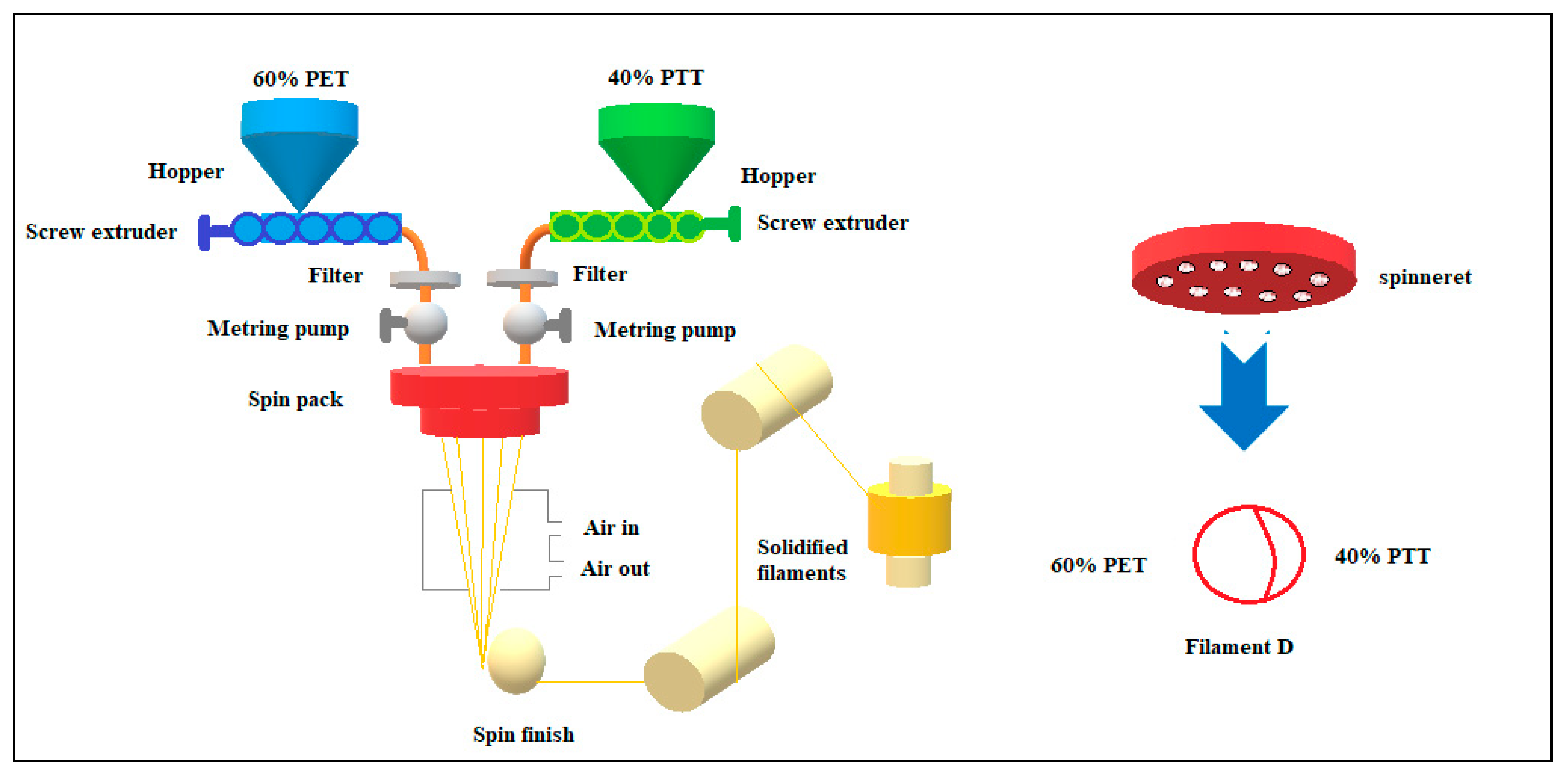
Figure 1.
Spinning process of bicomponent filaments using side by side configuration.
Figure 1.
Spinning process of bicomponent filaments using side by side configuration.
Figure 2.
Dyeing process (temperature Ti and time ti are parameters to be studied and optimized).
Figure 2.
Dyeing process (temperature Ti and time ti are parameters to be studied and optimized).
Figure 3.
Scanning electron micrographs of bicomponent filaments. (a,b) Configuration of filaments in the yarn; (c) Lengthwise view; (d) Cross section view.
Figure 3.
Scanning electron micrographs of bicomponent filaments. (a,b) Configuration of filaments in the yarn; (c) Lengthwise view; (d) Cross section view.
Figure 4.
IR spectra of bicomponent filaments.
Figure 4.
IR spectra of bicomponent filaments.
Figure 5.
Differential scanning calorimetry (DSC) spectrum of bicomponent filaments.
Figure 5.
Differential scanning calorimetry (DSC) spectrum of bicomponent filaments.
Figure 6.
Recovery elasticity of knitted samples made of 100% bicomponent filaments.
Figure 6.
Recovery elasticity of knitted samples made of 100% bicomponent filaments.
Figure 7.
Effect of dye bath pH on the color yield (K/S) of bicomponent filaments dyed with: (a) Dye #H; (b) Dye #M; (c) Dye #L (Temperature = 130 °C, Concentration of carrier = 0 g/L, Time = 50 min).
Figure 7.
Effect of dye bath pH on the color yield (K/S) of bicomponent filaments dyed with: (a) Dye #H; (b) Dye #M; (c) Dye #L (Temperature = 130 °C, Concentration of carrier = 0 g/L, Time = 50 min).
Figure 8.
Effect of dyeing temperature on the color yield (K/S) of bicomponent filaments dyed with: (a) Dye #H; (b) Dye #M; (c) Dye #L (pH = 7, Carrier concentration = 0 g/L, Time = 50 min).
Figure 8.
Effect of dyeing temperature on the color yield (K/S) of bicomponent filaments dyed with: (a) Dye #H; (b) Dye #M; (c) Dye #L (pH = 7, Carrier concentration = 0 g/L, Time = 50 min).
Figure 9.
Effect of dyeing time on the color yield (K/S) of bicomponent filaments dyed with: (a) Dye #H; (b) Dye #M; (c) Dye #L (pH = 7, Temperature = 130 °C, Concentration of carrier = 0 g/L).
Figure 9.
Effect of dyeing time on the color yield (K/S) of bicomponent filaments dyed with: (a) Dye #H; (b) Dye #M; (c) Dye #L (pH = 7, Temperature = 130 °C, Concentration of carrier = 0 g/L).
Figure 10.
Effect of carrier concentration on the color yield (K/S) of bicomponent filaments dyed with: (a) Dye #H; (b) Dye #M; (c) Dye #L (pH = 7, Temperature = 110 °C, Time = 50 min).
Figure 10.
Effect of carrier concentration on the color yield (K/S) of bicomponent filaments dyed with: (a) Dye #H; (b) Dye #M; (c) Dye #L (pH = 7, Temperature = 110 °C, Time = 50 min).
Figure 11.
Mains effects plots for color yield (K/S) of bicomponent filaments dyed with: (a) Dye #H; (b) Dye #M; (c) Dye #L.
Figure 11.
Mains effects plots for color yield (K/S) of bicomponent filaments dyed with: (a) Dye #H; (b) Dye #M; (c) Dye #L.
Figure 12.
Interactions plots for color yield (K/S) of bicomponent filaments dyed with: (a) Dye #H; (b) Dye #M; (c) Dye #L.
Figure 12.
Interactions plots for color yield (K/S) of bicomponent filaments dyed with: (a) Dye #H; (b) Dye #M; (c) Dye #L.
Figure 13.
Surface plots for color yield (K/S) of bicomponent filaments dyed with: (a) Dye #H; (b) Dye #M; (c) Dye #L.
Figure 13.
Surface plots for color yield (K/S) of bicomponent filaments dyed with: (a) Dye #H; (b) Dye #M; (c) Dye #L.
Table 1.
Physical characteristics of T400 multifilament yarn and knitted fabrics.
Table 1.
Physical characteristics of T400 multifilament yarn and knitted fabrics.
| Structures | Characteristics | Values | ISO Standards |
|---|
| T400 multifilament yarn | Composition of filament | 60% PET/40% PTT | --- |
| Number of filaments per yarn | 64 | --- |
| Average count of yarn (Tex) | 16.5 | ISO 7211/5 |
| Strength at break of yarn (N) | 5 | ISO 3377-2 |
| Elongation at break of yarn (%) | 25.41 | ISO 3377-2 |
| Fabric knitted with T400 multifilament yarn | Composition | 100% T400 multifilament yarn | --- |
| Type of binding | Jersey knit | --- |
| Knit thickness (mm) | 0.92 | ISO 5084 |
| Knit weight (g/m2) | 215 | EN 12127 |
| Strength at break (%) | 540 | ISO 13934-1 |
| Elongation at break (%) | 250 | ISO 13934-1 |
Table 2.
Chemical characteristics and configuration of studied disperse dyes.
Table 3.
Factors and levels used in the Box-Behnken experimental design.
Table 3.
Factors and levels used in the Box-Behnken experimental design.
| Factors | Units | Variation Levels |
|---|
| Low Level (−1) | Middle Level (0) | High Level (+1) |
|---|
| Dyeing temperature | °C | 110 | 120 | 130 |
| Dyeing time | min | 25 | 50 | 75 |
| Concentration of carrier | g/L | 0 | 6 | 12 |
Table 4.
The three-level Box-Behnken experimental design used in this study.
Table 4.
The three-level Box-Behnken experimental design used in this study.
| Run Order | Factors |
|---|
| Dyeing Temperature (°C) | Dyeing Time (min) | Carrier Concentration (g/L) |
|---|
| 1 | 110 | 25 | 6 |
| 2 | 130 | 25 | 6 |
| 3 | 110 | 75 | 6 |
| 4 | 130 | 75 | 6 |
| 5 | 110 | 50 | 0 |
| 6 | 130 | 50 | 0 |
| 7 | 110 | 50 | 12 |
| 8 | 130 | 50 | 12 |
| 9 | 120 | 25 | 0 |
| 10 | 120 | 75 | 0 |
| 11 | 120 | 25 | 12 |
| 12 | 120 | 75 | 12 |
| 13 | 120 | 50 | 6 |
| 14 | 120 | 50 | 6 |
| 15 | 120 | 50 | 6 |
Table 5.
ANOVA table of the color yield (K/S) for the studied parameters (R2(adj) = 92.32%, 99.83% and 94.83% for Dye #H, Dye #M, and Dye #L, respectively).
Table 5.
ANOVA table of the color yield (K/S) for the studied parameters (R2(adj) = 92.32%, 99.83% and 94.83% for Dye #H, Dye #M, and Dye #L, respectively).
| Dyes | Term | Effect | Coef. (Uncoded Data) | Coef. (Coded Data) | SE Coef. | F-Value | P-Value |
|---|
| Dye #H | Constant | - | −276.600 | 22.500 | 0.670 | 33.600 | 0.000 |
| A | 3.175 | 4.430 | 1.580 | 0.410 | 3.870 | 0.010 |
| B | 2.050 | 0.665 | 1.020 | 0.410 | 2.500 | 0.050 |
| C | −1.275 | 2.230 | −0.630 | 0.410 | −1.550 | 0.181 |
| A × A | −3.375 | −0.016 | −1.680 | 0.604 | −2.800 | 0.038 |
| B × B | −3.125 | −0.002 | −1.560 | 0.604 | −2.590 | 0.049 |
| C × C | −5.775 | −0.080 | −2.880 | 0.604 | −4.780 | 0.005 |
| A × B | −1.500 | −0.003 | −0.750 | 0.580 | −1.290 | 0.253 |
| A × C | −1.350 | −0.011 | −0.675 | 0.580 | −1.160 | 0.297 |
| B × C | −0.700 | −0.002 | −0.350 | 0.580 | −0.600 | 0.573 |
| Dye #M | Constant | - | −173.900 | 25.800 | 0.165 | 156.530 | 0.000 |
| A | 1.500 | 2.830 | 0.750 | 0.101 | 7.430 | 0.001 |
| B | 3.470 | 0.607 | 1.730 | 0.101 | 17.210 | 0.000 |
| C | 2.370 | 2.580 | 1.180 | 0.101 | 11.770 | 0.001 |
| A × A | −2.150 | −0.010 | −1.075 | 0.149 | −7.240 | 0.000 |
| B × B | −3.900 | −0.003 | −1.950 | 0.149 | −13.130 | 0.000 |
| C × C | −2.100 | −0.029 | −1.050 | 0.149 | −7.070 | 0.001 |
| A × B | −0.850 | −0.001 | −0.420 | 0.143 | −2.980 | 0.031 |
| A × C | −1.850 | −0.001 | −0.925 | 0.143 | −6.480 | 0.001 |
| B × C | −1.100 | −0.003 | −0.550 | 0.143 | −3.850 | 0.012 |
| Dye #L | Constant | - | −49.300 | 22.270 | 0.614 | 36.260 | 0.000 |
| A | 0.100 | 1.000 | 0.050 | 0.376 | 0.130 | 0.890 |
| B | 1.300 | 0.236 | 0.650 | 0.376 | 1.730 | 0.145 |
| C | −3.100 | 1.780 | −1.550 | 0.376 | −4.120 | 0.009 |
| A × A | −0.827 | −0.004 | −0.410 | 0.554 | −0.750 | 0.489 |
| B × B | −1.927 | −0.001 | −0.963 | 0.554 | −1.740 | 0.142 |
| C × C | −8.827 | −0.122 | −0.410 | 0.554 | −7.970 | 0.001 |
| A × B | 0.000 | 0.000 | 0.000 | 0.532 | 0.000 | 1.000 |
| A × C | −0.100 | −0.000 | −0.050 | 0.532 | −0.009 | 0.929 |
| B × C | −2.800 | −0.009 | −1.400 | 0.532 | −2.630 | 0.046 |
Table 6.
Optimal conditions obtained by Box-Behnken design and the corresponding theoretical K/S values of samples dyed with used dyes.
Table 6.
Optimal conditions obtained by Box-Behnken design and the corresponding theoretical K/S values of samples dyed with used dyes.
| Dyes | K/S | Dyeing Temperature (°C) | Dyeing Time (min) | Concentration of Carrier (g/L) |
|---|
| Dye #H | 23.03 | 124.55 | 55.80 | 4.96 |
| Dye #M | 26.41 | 120.90 | 59.34 | 8.60 |
| Dye #L | 22.60 | 117.53 | 62.87 | 4.48 |
Table 7.
Obtained values of color yield (K/S) and colorimetric coordinates 1 (in D65/10°) of samples dyed with used dyes under optimum dyeing conditions.
Table 7.
Obtained values of color yield (K/S) and colorimetric coordinates 1 (in D65/10°) of samples dyed with used dyes under optimum dyeing conditions.
| Dyes | K/S | L* ± ΔL* | a* ± Δa* | b* ± Δb* | C* ± ΔC* | ΔECMC(2:1) 2 |
|---|
| Dye #H | 23.18 | 29.37 ± 0.32 | 46.91 ± 0.26 | 6.00 ± 0.21 | 47.29 ± 0.32 | 0.46 |
| Dye #M | 26.32 | 73.63 ± 0.16 | 11.09 ± 0.30 | 46.51 ± 0.09 | 47.81 ± 0.10 | 0.35 |
| Dye #L | 22.25 | 33.50 ± 0.47 | 56.68 ± 0.20 | 6.69 ± 0.39 | 57.07 ± 0.24 | 0.64 |
Table 8.
Colorfastness of bicomponent filaments dyed with used dyes under optimum dyeing conditions.
Table 8.
Colorfastness of bicomponent filaments dyed with used dyes under optimum dyeing conditions.
| Dyes | Wash Fastness
(ISO 105-C06) | Crock Fastness
(ISO 105-X12) | Light Fastness
(ISO 105-B02) |
|---|
| Staining | Color Change | Dry | Wet |
|---|
| Dye #H | 5 | 4–5 | 5 | 4–5 | 8 |
| Dye #M | 4 | 4 | 4–5 | 4–5 | 7–8 |
| Dye #L | 4 | 4 | 4 | 3–4 | 7–8 |
Table 9.
Obtained results of elongation at break, strength at break, recovery elasticity, and permanent deformation of bicomponent filaments knitted samples before and after dyeing under optimum conditions.
Table 9.
Obtained results of elongation at break, strength at break, recovery elasticity, and permanent deformation of bicomponent filaments knitted samples before and after dyeing under optimum conditions.
| Samples | Elongation at Break (%) | Strength at Break (N) | Recovery Elasticity after 1 Cycle (%) | Recovery Elasticity after 5 Cycles (%) | Permanent Deformation (%) |
|---|
| Before dyeing | 309.40 | 538.03 | 79.80 | 59.98 | 50.02 |
| After dyeing with Dye #H | 278.66 | 584.06 | 80.80 | 60.36 | 49.55 |
| After dyeing with Dye #M | 292.76 | 569.25 | 80.72 | 60.27 | 49.66 |
| After dyeing with Dye #L | 277.16 | 571.13 | 80.92 | 60.41 | 49.48 |

 ,
, 


