Article

Answer Set Programming for Computing Constraints-Based Elementary Flux Modes: Application to Escherichia coli Core Metabolism

1
LRI, Université Paris-Saclay, CNRS, 91405 Orsay, France
2
Department of Chemical and Biological Engineering, Center for Biofilm Engineering, Microbiology and Immunology, Montana State University, Bozeman, MT 59717, USA
3
INRAE, UR1404, MaIAGE, Université Paris-Saclay, 78350 Jouy-en-Josas, France
*
Author to whom correspondence should be addressed.
Processes 2020, 8(12), 1649; https://doi.org/10.3390/pr8121649
Submission received: 13 November 2020 / Revised: 4 December 2020 / Accepted: 8 December 2020 / Published: 14 December 2020

Abstract

:
Elementary Flux Modes (EFMs) provide a rigorous basis to systematically characterize the steady state, cellular phenotypes, as well as metabolic network robustness and fragility. However, the number of EFMs typically grows exponentially with the size of the metabolic network, leading to excessive computational demands, and unfortunately, a large fraction of these EFMs are not biologically feasible due to system constraints. This combinatorial explosion often prevents the complete analysis of genome-scale metabolic models. Traditionally, EFMs are computed by the double description method, an efficient algorithm based on matrix calculation; however, only a few constraints can be integrated into this computation. They must be monotonic with regard to the set inclusion of the supports; otherwise, they must be treated in post-processing and thus do not save computational time. We present aspefm, a hybrid computational tool based on Answer Set Programming (ASP) and Linear Programming (LP) that permits the computation of EFMs while implementing many different types of constraints. We apply our methodology to the Escherichia coli core model, which contains 226 × 10 6 EFMs. In considering transcriptional and environmental regulation, thermodynamic constraints, and resource usage considerations, the solution space is reduced to 1118 EFMs that can be computed directly with aspefm. The solution set, for E. coli growth on O2 gradients spanning fully aerobic to anaerobic, can be further reduced to four optimal EFMs using post-processing and Pareto front analysis.

1. Introduction

Understanding the structure and function of biochemical networks is an essential step in characterizing cellular capabilities. The use of reconstructed, genome-enabled, metabolic models has been widely applied in systems biology to study cellular metabolism. Approaches based on stoichiometric analysis, such as Elementary Flux Mode (EFM) analysis [1,2], are powerful methods for describing the mass balanced operation of metabolic networks. A metabolic network composed of m metabolites and r reactions can be represented by a stoichiometry matrix S with m rows and r columns, where coefficients S i j take value k if reaction j produces k units of metabolite i, k if reaction j consumes k units of metabolite i and 0 otherwise. A mode is a flux vector ν R r such that S ν = 0 and ν j 0 j I r r e v , with I r r e v the set of irreversible reactions in this network. The support of a mode is the set of reactions with a non-zero flux: S u p p ( ν ) = { i | ν i 0 } . A mode e is an EFM if its support is minimal by inclusion, i.e., there does not exist e 0 such that S u p p ( e ) S u p p ( e ) . EFMs can be defined as the smallest sub-networks enabling the metabolic system to operate at steady state with all irreversible reactions proceeding in the appropriate direction. Such a pathway definition provides a rigorous basis to systematically characterize metabolic phenotypes, network robustness and fragility, and facilitate the understanding of cellular physiology. EFMA fully characterizes the metabolic capabilities of an organism since every steady state flux can be represented as a non-negative linear combination of EFMs. This property is useful in many applications such as in analyzing the stability of metabolic systems [3,4], or in identifying gene deletions that are lethal to the network [5,6], or in designing optimal cell factories [7,8].
Most microbial habitats are dynamic, and the availability of resources like electron donors, electron acceptors, and anabolic forms of nitrogen can change with time. Phenotypic plasticity, where the utilized metabolic pathways change with the changing environment, permits microorganisms to remain competitive. Analyzing potential metabolic strategies in the phenotypic tradeoff space permits the identification of EFMs that are competitive for gradients of resource scarcity. EFM analysis of E. coli phenotypic acclimation to gradients of resource availability, including O2 and anabolic nitrogen, have been reported using tradeoff analysis and Pareto optimization [9,10,11,12]. The methodology tabulates the resource requirements to realize each EFM; these resources can be anabolic, e.g., nitrogen to assemble metabolic enzymes, which are described here as resource investment costs or catabolic, e.g., O2 which serves as an electron acceptor, which are described here as resource operating costs. Some resources can serve both anabolic and catabolic functions like glucose which is both an energy source and carbon source for enzyme synthesis. Optimal phenotypes for acclimating to environments along gradients of resource scarcity can be identified by plotting the resource costs for each EFM in a tradeoff space where Pareto optimality identifies the most competitive phenotypes [13]. Those EFMs that minimize the resource requirements to achieve a target cellular function are considered most competitive because the phenotypes would permit the most biomass to be made based on a finite supply of a substrate. Tradeoff analysis has accurately predicted and interpreted E. coli acclimation to O2, carbon, and nitrogen, scarcity based on physiological, proteomics, and fluxomics data from E. coli chemostat cultures [14,15].
The optimal solution of a constraint-based enzyme allocation problem, with general kinetics, is an EFM [16]. Wortel et al. [17] studied growth rate vs. growth yield tradeoffs using an Enzyme-Flux Cost Minimization (EFCM) method. All biomass producing EFMs were screened and it was assumed that the growth rate depended linearly on the enzyme investment per rate of biomass production. EFMs can also be used for dynamic metabolic modeling such as macroscopic biochemical reaction models [18] or hybrid cybernetic models [19]. In these cases, the enumeration of all EFMs is not needed, but the enumeration of EFMs of interest is essential. Traditionally, EFMs are computed by the Double Description (DD) algorithm [20,21], an efficient algorithm based on matrix calculation. Well-known implementations of DD algorithm for computing all the EFMs in a network include METATOOL [22] and EFMTool [23]. However, the number of EFMs typically grows exponentially with the size of the network. Methods based on a network splitting algorithm allow the computation of ∼2 billion EFMs from a large metabolic model of microalga Phaeodactylum tricornutum consisting of 318 reactions [24] while, many genome-scale networks have on order of thousands of reactions. Thus, it is not currently possible to enumerate all EFMs from most genome-scale metabolic models. Another inherent problem is finding EFMs of interest from the large solution set. Among the many EFMs computed, only a small fraction are thought to be active in cells. To save computational time and memory and to focus on biologically relevant phenotypes, it becomes necessary to integrate biological constraints directly during the computation of EFMs.
It is possible to integrate constraints during the calculation of EFMs using the DD algorithm, however the constraints must be monotonic with regard to the set inclusion of the supports; i.e., if a given flux distribution of support S verifies the constraints, so it is for any flux distribution with support included in S [25,26]. Thermodynamic constraints, which are monotonic on the support, have been integrated into the tEFMA tool [27,28] which uses the DD algorithm to obtain the EFMs compatible with the negative Gibbs free energy constraint. This is achieved by interfacing efmtool [23] with the Linear Program tool CPLEX. By using Farkas duality, we have proposed a method (thermoEFM) to compute EFMs consistent with the equilibrium constants. This method was used to orient the direction of flux in reversible EFMs and it only requires knowledge of the concentrations of external metabolites and the equilibrium constants for each reaction [26]. We showed that these thermodynamic constraints can even be checked directly within the DD framework by adding a supplementary linear, non-negativity constraint [29].
Boolean constraints, such as transcriptional regulation constraints, are less favorable to use with the DD algorithm since most constraints are not support monotone except for the negative clauses (inhibition of reactions). In particular, RegEFMtool [25] integrates negative clauses during the incremental process of the DD algorithm and has to treat all other constraints in post-processing. This was the motivation to apply logic methods such as Satisfiability Modulo Theories (SMT) to compute EFMs consistent with regulatory constraints [30,31]. This approach can integrate all types of Boolean constraints even if they are not support-monotone. However, the flux cone is restructured depending on the constraints and the minimal generating vectors of the constrained cone, called Minimal Constraint Flux Modes (MCFM) [31], are not always EFMs and may be a combination of EFMs from the unconstrained cone.
To enumerate only a subset of EFMs, de Figueireido et al. [32] proposed the k-shortest EFMs, a Mixed Integer Linear Programming (MILP) method that lists the shortest EFMs up to an iteration k, k which is the number of nonzero flux reactions in the EFM. This method has been revisited several times [33,34], in particular for other applications such as GFMs (Generating Flux Modes, subset of EFMs) [35], Minimal Cut Sets (MCSs) [36], an application of EFMs that allows one to identify essential reactions within a metabolic network, and to compute EFMs containing a given set of target reactions [37]. Another variation termed Alternate Integer Linear Programming (AILP) was proposed by Song et al. for computing EFMs and MCSs in a sequential manner [38]. Both the SMT and MILP methods can enumerate EFMs on the fly on large models (defined here as networks with ∼200+ reactions), for which the DD algorithm may not work.
Answer Set Programming (ASP) is a widely used tool in logical programming. It has been utilized to solve a variety of biological problems including metabolic network problems. Gebser et al. [39] used this formalism to check the consistency of large-scale data sets and provided explanations for inconsistencies by determining minimal representations of conflicts. Razzaq et al. [40] combined ASP and model checking to integrate time series of phosphoproteomic data into protein signaling networks. More recently, Frioux et al. [41] developed a hybrid ASP and linear programming approach for the network gap-filling problem using the solver clingo[LP] [42], an extension of the state-of-the art ASP solver clingo [43] for solving logic problems with linear constraints over integer and real numbers.
Inspired by this formalism, aspefm, a new hybrid ASP method with clingo[LP], was developed for computing EFMs under Boolean and linear constraints. As SMT and MILP, the computation of EFMs in ASP aims to enumerate EFMs upon request from large networks. However, the use of logical programming with linear constraints provides a method for enforcing numerous types of biological constraints including transcriptional and environmental regulation, thermodynamics, and resource operating costs on the computation of EFMs, all with a human-readable format.
To show its versatility, our aspefm tool was applied to a well-known E. coli core model with a significant number of EFMs. The method proved capable of computing a subset of biologically-relevant EFMs while a Pareto front optimization was performed as a final analysis step. The framework returned a small number of EFMs which could be analyzed manually and compared with experimental data.

2. Results

2.1. Application on the E. coli core Model

The aspefm method was applied to the E. coli core model by Orth et al, 2010, which includes a full transcriptional regulation network, as well as thermodynamic equilibrium data [44]. The E. coli core metabolic network consisted of 95 reactions, 72 internal metabolites, 20 external metabolites, and 78 regulation rules. Fifty-nine reactions were reversible. The core model was found to contain 226.6 × 10 6 EFMs based on a previous study [25].
The ASP-based EFMA tool computed a biologically relevant subset of EFMs belonging to this network by integrating thermodynamic and regulatory constraints. Additionally, the simulations considered environmental constraints based on growth in a minimal medium containing glucose, CO2, NH 4 + , inorganic phosphate, H+, H2O and O2. Accordingly, all other transport reactions were inactivated. The biomass-producing EFMs were selected to represent cellular growth. To further reduce computational burden, the solution space was limited to EFMs with a O2 operating cost of less than 0.7 O2 moles per biomass C mole and a glucose operating cost of less than seven glucose C moles per biomass C mole. Since the presence of O2 had a large impact on the regulatory constraints, two separate scenarios were considered: (1) aerobic and (2) anaerobic conditions.
The ASP-based tool identified 1118 aerobic and 363 anaerobic EFMs in 542 s and 232 s, respectively (Table 1). The tool also returned 39 aerobic MCFMs that were filtered out in post-processing. Results were obtained on a commercial laptop with Intel® Core™ i5-7440HQ CPU 2.80 GHz.
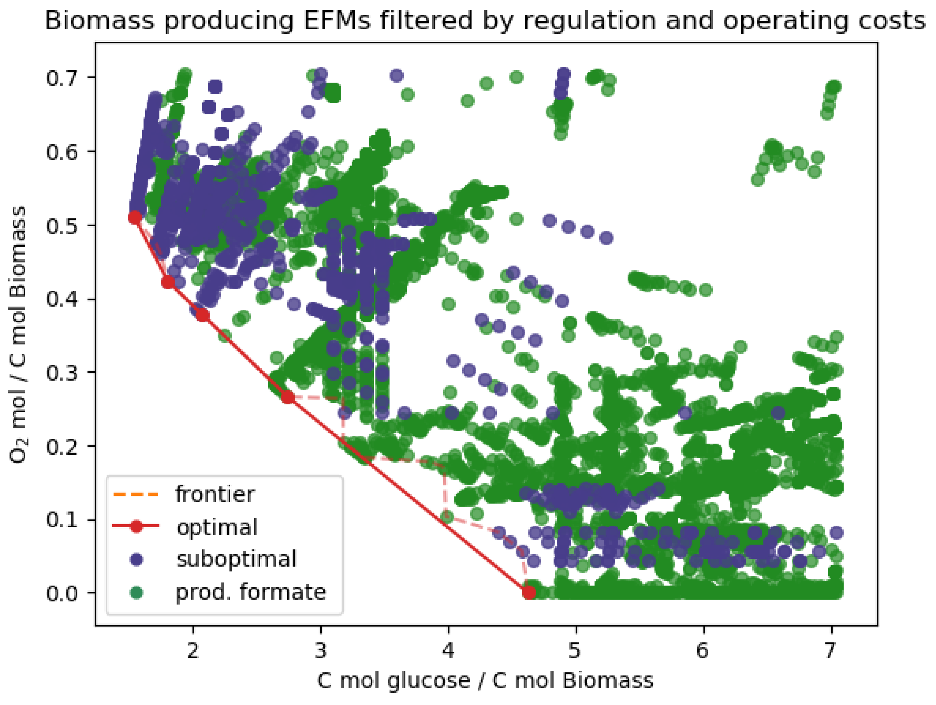
The aggregate set of aerobic and anaerobic EFMs was processed using a phenotypic tradeoff analysis with Pareto optimization of biomass production relative to O2 availability, as described previously in Carlson and Srienc, 2004 [9]. EFMs that permitted optimal acclimation to gradients of O2 scarcity had the lowest substrate operating costs (C moles glucose consumed/C mole biomass produced and moles O2 consumed/C mole biomass produced) defining a Pareto front. Four EFMs defined the Pareto surface with the applied constraints (Figure 1, Appendix A).

2.2. Model Modifications

The regulation network applied in Orth et al. [44] was examined for refinement. A modification to formate metabolism was made based on experimental data. Formate has been measured in E. coli cultures in the presence of O2. The pyruvate formate lyase (PFL) enzyme, which produces formate, is O2 sensitive, but activity is possible when dissolved O2 concentrations are low, as occurs when cells grow rapidly or in high density cell cultures [14,15,45,46]. In the regulation network, the PFL enzyme was disabled in the presence of O2 by transcriptional regulators ArcA and FNR. Removing this regulation rule for formate metabolism resulted in a ∼10-fold increase in the number of total EFMs (Table 1) and a slightly different Pareto front, which predicted formate production at low O2 availability (Figure 2), consistent with experimental data and previous EFM analyses [9,14,15,46]. Briefly, the Pareto front included the most efficient EFM for producing biomass from glucose, the upper left EFM, which also had a relatively high O2 requirement. As environmental O2 availability decreases, optimal use of the network shifts right along the Pareto front quantifying the increased requirement for glucose as metabolic byproducts are secreted. The first predicted byproduct moving down the Pareto surface was acetate, followed by a combination of acetate and formate and, finally, under anaerobic conditions acetate, formate and ethanol.
The E. coli core model was originally formulated for Flux Balance Analysis (FBA) [47] and the biomass synthesis reaction did not include maintenance energy. The biomass reaction was modified to facilitate its integration with EFMA by account of the maintenance energy required for a culture with a 40 min doubling time. The biomass reaction was also updated to create a biomass elemental stoichiometry, including the degree of reduction, consistent with experimental measurements. A detailed explanation of the modifications and additional results are provided in Appendix B and Appendix C.

3. Discussion

The presented aspefm method greatly improves the calculation of constraint-based EFMs. It is capable of enumerating the EFMs of interest without having to calculate and store the complete set of EFMs and it negates the requirement for secondary processing required to select the desired subset. Indeed, E. coli core contained 226.6 × 10 6 EFMs (251 GB) which were computed using EFMtool in 34.1 h [25]. When the regulation network rules were considered, using tool RegEFMTool, the number of EFMs dropped to 2.1 × 10 6 (2.3 GB) with a run time of 7.1 h. The substantial requirement for disk space to store the complete set of EFMs hampered further analysis. In contrast to these DD-based methods, aspefm makes it possible to integrate a large number of constraints reducing the calculation of non-relevant EFMs. The ASP-based method calculates the desired EFMs relatively quickly without the need for huge storage capacity. In addition, while FBA-based problems are often easily solved, they typically only identify solutions when the constraints make the solution space convex. For example, when stoichiometric and thermodynamic constraints are considered together, the set of possible flux configurations does not generally define a convex set, and thus, it is generally difficult to solve with FBA-relevant optimization algorithms, contrary to the presented analysis. See [48] for a review that tackles the different class of problems.
It is worth noting that computing a minimal set of EFMs with constraints is fundamentally different from computing EFMs and filtering them. In our previous work, we established that the set of EFMs satisfying a constraint c does not always match with the set of flux distributions at the steady state of minimal support satisfying c, which we coined as Minimal Constrained Flux Modes (MCFMs) [31]. In particular, this is the case when c is an additional linear constraint ν 1 + ν 2 > 0 , or alternately, a conjunction of positive Boolean literals z 1 z 2 . Steady state solutions of minimal support for such a constraint c (i.e., MCFMs) may be combinations of several EFMs. These MCFMs can be easily discarded by a kernel test. A solution vector S o l is a MCFM and not an EFM if d i m ( K e r ( S S u p p ( S o l ) ) ) 1 [49]. In other cases, the set of MCFMs would correspond exactly to the set of EFMs satisfying the constraint. For example, disjunctions of negative literals do not impact the decomposability of solutions. When we bound the operating cost of several metabolites, we add linear constraints in the set of ASP rules which can generate MCFMs which are not EFMs. This is the case in our analysis of the E. coli core model, but their number is small compared to the total number of EFMs (39 MCFMs filtered out versus 1118 EFMs with the standard regulation and 119 MCFMs filtered out versus 11,017 EFMs with the revised formate regulation, see Table 1 and the additional results in Appendix D).
This work highlights the importance of integrating different types of constraints when performing EFMA on a metabolic model. First, integration of strict Boolean constraints allows the user to restrict analysis to a specific environment and to consider the effects of transcriptional regulation. However, as illustrated by the presented formate metabolism regulation of the E. coli core model, a transcriptional regulation network that is too stringent might lead to the omission of experimentally relevant pathways. Second, the integration of curated thermodynamic data enables the computation of EFMs consistent with the equilibrium constants. Conversely, thermodynamic data can be overly lenient, as is the case in this analysis where no EFMs were filtered from the set. Finally, when analyzing biomass production, the application of substrate operating costs bounds constrained the enumerated EFMs to biologically reasonable ranges, but the process may have generated unwanted MCFMs, which had to be removed. Biomass operating costs are convenient for performing Pareto front analyses, which, in turn, facilitate the comparison of model results with experimental data.
The presented results are promising as they expand substantially the range of model sizes that can be decomposed into EFMs. However, in order to be applied to large-scale models, the tool will likely require a large number of biological constraints. Otherwise, clingo[LP] may struggle with the number of linear problems that need to be solved. Boolean constraints work notably well since clingo[LP] is primarily a logic solver, and Boolean constraints mean cutting solutions early before solving any linear problems. The current standard for metabolic models is to link genes to reactions through Boolean associations [50]. clingo[LP] is a very efficient tool for solving these Boolean constraints while still representing the syntax in a readable format; and thus, many models found on the BiGG database [51], could be analyzed with our tool using only a reasonable number of additional constraints.
The computation time could be further improved via network reduction and using multi-thread computation routines. The ASP-based implementation with clingo[LP] does not currently use multi-threading, so computing EFMs on a server would have minimal benefit in terms of computing time. The method is compatible with network reduction techniques such as the enzyme subsets’ (i.e., groups of enzymes that operate together in fixed flux ratios at steady state) computation as described in [1,52], although in this case, only the reduced reactions and metabolites should be used as the input metabolic network. Applied constraints would need to be cast in a manner consistent with the reduced network representation. The network reduction process, including appropriate translation of regulatory constraints, will be the focus of future work.

4. Materials and Methods

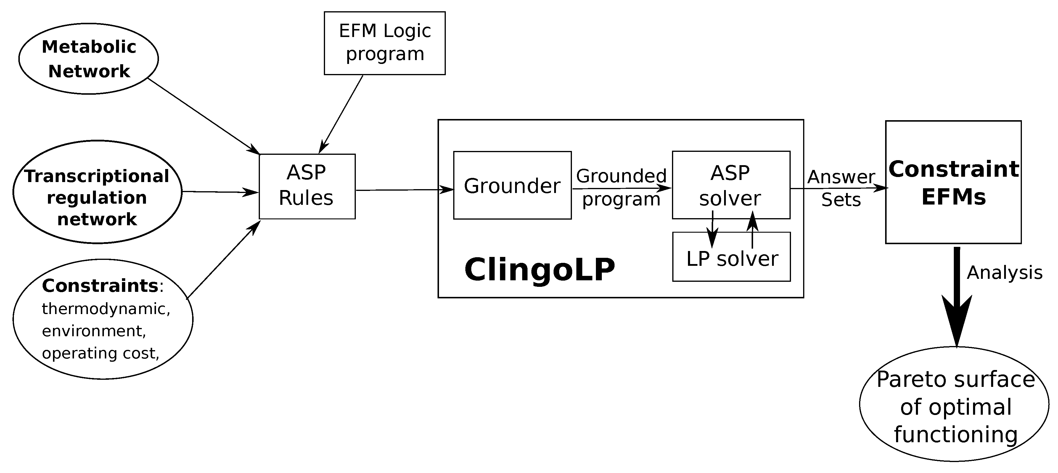
The aspefm method makes use of a metabolic network and biological constraints translated into a set of ASP rules and integrates them into the hybrid ASP and LP solver clingo[LP] to compute constraint-based EFMs. Finally, the resulting EFMs can be processed with a Pareto surface analysis. An overview of the framework is presented in Figure 3. The necessary files to run the analysis on the E. coli core network are provided in Supplementary Files S4 and S5 and described in Appendix F and Appendix G.

4.1. Answer Set Programming

Answer Set Programming (ASP) is a declarative approach oriented toward knowledge processing with a logic programming approach. Problems are formulated according to first-order propositional logic in order to facilitate the problem modeling. A logic program in ASP is a finite set of rules of the form:
a b 1 , , b m , n o t c m + 1 , , n o t c n
where a , b 1 , , b m , c m + 1 , c n are atomic propositions. An atom a either belongs in a program solution or not, in which case it is denoted by n o t a . Closed-world assumption applies, meaning that by default atoms do not belong to a solution. The head of a rule denotes atom a and the body denotes positive atoms b 1 , , b m and negative atoms c m + 1 , c n . If all positive body atoms are present and all negative body atoms are absent then the head atom should be present. To state that an atom should be present in the solution, the body is omitted. This is called a fact. Alternatively, to state integrity constraints on body atoms, the head atom is omitted. A typical ASP tool is composed of two parts: the grounder which handles predicate variables and the solver which finds stable sets of atoms satisfying the logic program. For a complete formal introduction to answer set programming, we refer the reader to [53].
The software clingo from the University of Potsdam performs ASP grounding and solving. Its solver takes advantage of high performance solving using Boolean satisfiability (SAT) resolution techniques [54]. In the latest version, clingo has been extended with theory reasoning capacities [43]. It allows for tools such as clingo[LP], which can handle linear constraints in an ASP logic program [42]. We use clingo[LP] with strict semantics and the linear programming solver CPLEX.

4.2. Problem Formulation of EFMs Computation

Let us represent a metabolic network by a quintuplet N = ( M , R , S , E x t , R e v ) with M a set of metabolites, R a set of irreversible reactions, S a stoichiometric matrix of size | M | × | R | , E x t M the subset of external metabolites, and R e v : R × R the set of all pairs ( r , r r e v ) of reactions such that r and r r e v are issued from the splitting of a reversible reaction. We denote by s m r the stoichiometric coefficient from S associated with metabolite m and reaction r.
Using this formalism, we define a set of hybrid predicate logic and linear constraints on the network to be encoded into a set of ASP rules in the clingo[LP] syntax. Given a reaction r, we represent its flux by the variable ν r and if it is active by the Boolean indicator variable z r { 0 , 1 } . Since all reactions are irreversible, this means all fluxes have non-negative values. In order to be a flux vector at steady-state, a solution should satisfy the following constraints on variables ν r and z r :
ν r 0 r R
z r ν r > 0 r R
¬ z r ¬ z r r e v ( r , r r e v ) R e v
r R z r
r R s m r × ν r = 0 m M E x t
Notice that Equations (1), (2) and (5) need the likes of a linear programming solver, while the other equations are solved with propositional logic only. Equation (1) ensures that all fluxes are non-negative values. Equation (2) ensures that the Boolean indicator variables are true if and only if the flux has a strictly positive value. Equation (3) ensures that the resulting flux does not contain both directions of a split reversible reaction. Equation (4) excludes the trivial solution, and the steady state assumption is fulfilled by Equation (5). These program rules and the metabolic networks are expressed in ASP using the predicates presented in Appendix E.
The problem formulation is reminiscent of the k-shortest EFMs method. In the MILP problem, on top of these rules, the solver is given the task to minimize the sum of indicator variables, thus returning the shortest flux modes. In our method, such a minimization was not considered. Instead, clingo allows us to set heuristics to enumerate answer sets that are a subset minimal in regards to the indicator variables [55]. This gives us flux solutions with subset minimal support or elementary flux modes. In summary, we are able to enumerate the EFMs of a given input metabolic network by translating the network and the rules presented above into a clingo[LP] logic program and by using clingo heuristics.

4.3. Constraints’ Formulation

A major functionality of our tool is the ability of computing EFMs under a variety of constraints. This is done directly during the computation without the filtering step in post-processing. As in some cases, the flux modes computed under constraints may be different from elementary modes, we will not refer to them directly as such. We characterize two different types of constraints: logical constraints and linear constraints. While logical constraints are handled by clingo alone, linear constraints are ultimately solved by the linear programming solver. Since standard linear programming does not support logical constraints well, we aim to propose an approach that can handle all types of constraints. Any additional set of logical and linear constraints can be given as input to our encoding using clingo[LP]. When given to clingo alongside the input network and the problem rules, the solver will compute directly the EFMs under constraints (Figure 3). Biologically relevant constraints tested with our tool include transcriptional and environmental regulation (6) and (7), thermodynamic equilibrium (8) and biomass operating cost (9).
Let us denote by R e g the set of Boolean variables corresponding to transcriptional regulation constraints. A Boolean function f ( R e g ) on these variables is any Boolean expression that may be formed from the variables and NOT, AND, and OR logic operators. Using this formalism, we say that a reaction r is active only if its regulation rule f r ( R e g ) returns true (Equation (6)).
z r f r ( R e g ) r R
For example, the regulation for a transport reaction t s p A may be z t s p A A e x t r e g t s p A where Boolean variable A e x t R e g indicates the presence of external metabolite A E x t and Boolean variable r e g t s p A R e g indicates the presence of transcriptional regulator r e g t s p A . The truth values of Boolean variables can either be automatically inferred with other Boolean functions provided in the transcriptional regulation network or manually set before starting the computation of EFMs.
In practice, following from the formalism proposed by Covert and Palsson [56], we introduce Boolean variables for every external metabolite and add regulation rules for each transport reaction (Equation (7)), providing us with full control of the environments and environmental regulation. This is a crucial step as restricting us to a single environment reduces drastically the number of EFMs.
z t s p E e x t t s p R , E E x t such that s E · t s p < 0
An EFM e is consistent with the thermodynamic equilibrium if e T ln K ^ e q > 0 [26] with K ^ e q the vector of apparent equilibrium constants such that for each reaction j: K ^ e q j = K e q j i [ E X i ] S ( i , j ) . Apparent equilibrium constants are calculated from standard reaction equilibrium constants, external metabolite stoichiometry, and external metabolite concentrations. This constraint is expressed very simply in our formalism for ASP (Equation (8)).
r R ν r × ln K ^ e q r > 0
Adding an upper bound on the operating cost further restricts the solution space. It is expressed as a linear constraint (Equation (9)). For example, we say that the O2 flux must be inferior to 30 times the biomass flux: ν t s p O 2 < 30 ν B I O M A S S . Considering there are about 42.5 C moles in the E. coli core biomass, this results in taking the EFMs, the oxygen operating cost of which is less than 0.7 O2 moles per biomass C mole.
α ν r 1 < β ν r 2 r 1 R , r 2 R , α R , β R

4.4. Pareto Surface of Optimal Functioning

An analysis of the bidimensional operating cost space was performed as described in [9] to identify the most efficient EFMs for converting substrates into biomass. The technique found Pareto optimal EFMs, specific EFMs that minimized operating costs for both substrates of interest: Glucose and O2, and that defined in aggregate, a surface of optimal functioning.
The analysis was based on the assumption that evolution has selected phenotypes, represented by EFMs, that minimize both operating costs simultaneously. Cells expressing phenotypes that do not minimize both costs would not produce as much biomass as cells that do, limiting their fitness in the considered environment. EFMs (or linear combinations of the EFMs) found along the edge of the bidimensional substrate operating cost space represent optimal phenotypes for growth on glucose and a gradient of O2 availability spanning sufficiency to anaerobic conditions.
The method to identify the EFMs that were Pareto optimal, with respect to both operating costs, computed the convex hull of the operating cost space of EFMs. A solution ν * S o l s is said to be Pareto optimal with respect to cost functions f i for all i if and only if:
ν S o l s such that f i ( ν ) f i ( ν * ) for all i and f i ( ν ) < f i ( ν * ) for at least one i

5. Conclusions

We describe aspefm, a new method for calculating constraint-based EFMs based on answer set programming and linear programming. This method permits the integration of varied types of constraints, which reduce the solution space, enabling the enumeration of biologically relevant EFMs from large metabolic networks. We apply this tool to the E. coli core metabolism model, which contains a very large number of EFMs. Despite this, aspefm successfully identifies, what are deemed to be, all biologically relevant EFMs for producing biomass in a minimal glucose medium. A Pareto optimality analysis is then performed to identify the most efficient phenotypes, represented by EFMs, for cellular growth on a gradient of O2 availability spanning sufficiency to anaerobic conditions. The tool greatly expands the size range of metabolic models that can be analyzed for EFMs and, thus, greatly expands the potential for using EFMs to interpret complex biological behaviors.

Supplementary Materials

The following are available online at https://www.mdpi.com/2227-9717/8/12/1649/s1, File S1: Pareto optimal pathways of the E. coli core, File S2: E. coli core Biomass modifications, File S3: Pareto optimal pathways of the E. coli core with the adjusted biomass, File S4: ASP programs, File S5: Additional Python code.

Author Contributions

Conceptualization, M.M. and S.P.; methodology, M.M., R.P.C. and S.P.; software, M.M.; validation, M.M., R.P.C. and S.P.; formal analysis, M.M. and S.P.; writing—original draft, M.M., R.P.C. and S.P.; supervision, S.P. All authors have read and agreed to the published version of the manuscript.

Funding

R.P.C. was supported by the National Institutes of Health Award U01EB019416.

Conflicts of Interest

The authors declare no conflict of interest.

Abbreviations

The following abbreviations are used in this manuscript:
EFMElementary Flux Mode
EFMAElementary Flux Modes Analysis
FBAFlux Balance Analysis
DDDouble Description
ASPAnswer Set Programming
LPLinear Programming
SMTSatisfiability Modulo Theories
MCFMMinimal Constrained Flux Mode
MILPMixed Integer Linear Program

Appendix A. Pareto Optimal Pathways of E. coli

The Pareto optimal pathways for the E. coli core model were visualized in HTML format with the tool Escher [57]. We represent a total of five EFMs for the network without formate regulation. The pathways for both regulation conditions are presented in a ZIP file attached in Supplementary File S1.

Appendix B. E. coli Biomass Modifications

The E. coli core biomass coefficients were modified so that they included ATP maintenance requirements. The biomass now required 139 moles of ATP, for an amount of 42.55 C moles of biomass and an E. coli doubling time of 40 min.
We also modified accordingly the H + and H2O coefficients in order for the number of electrons and hydrogen and oxygen moles in the biomass to be closer to typical E. coli values. The calculations are detailed in the Excel file attached in Supplementary File S2.

Appendix C. Pareto Optimal Pathways of E. coli with the Adjusted Biomass

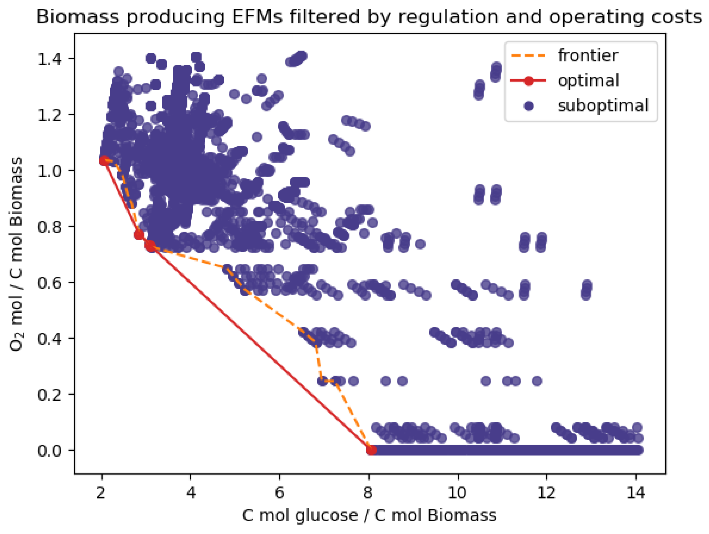
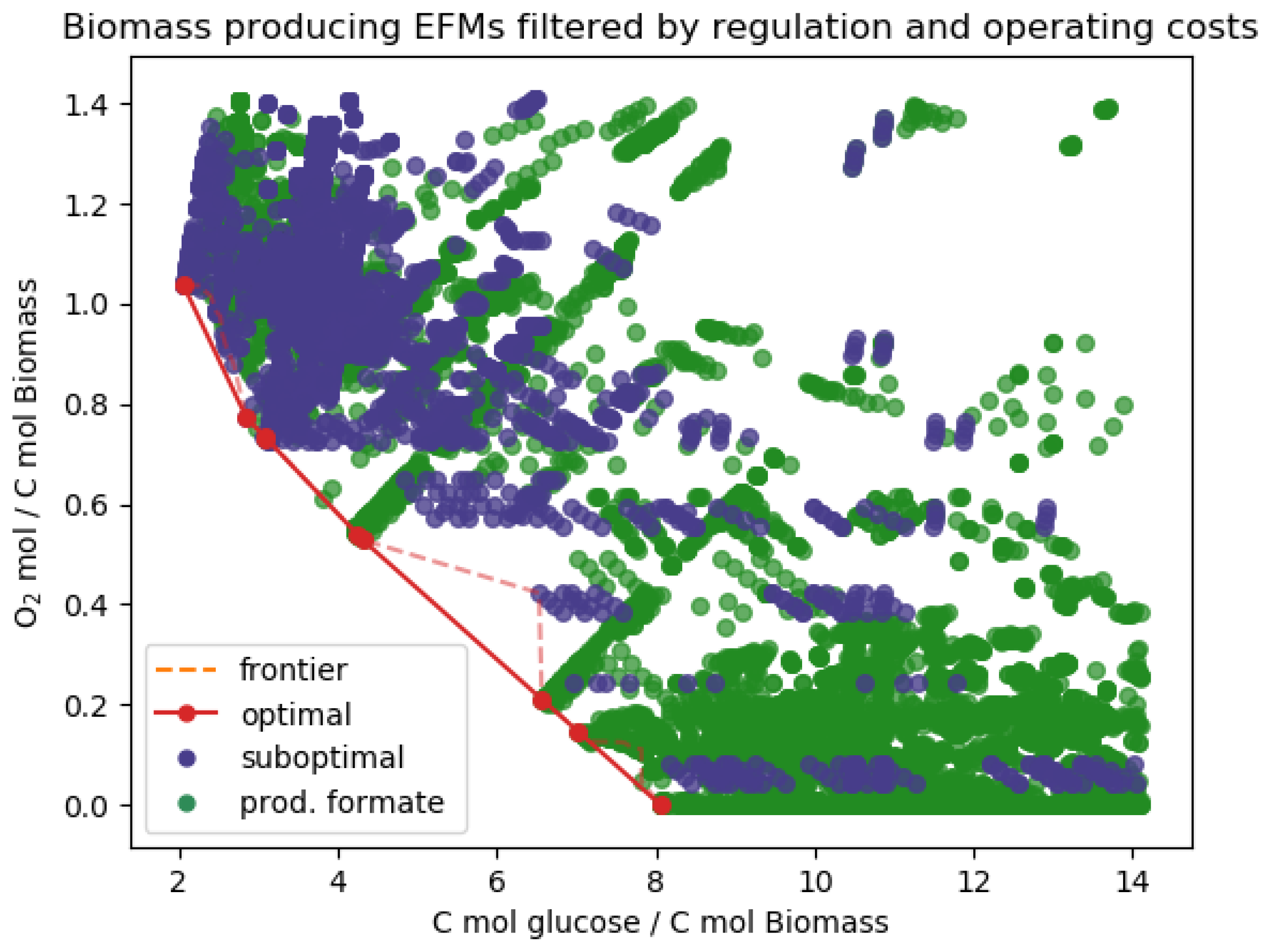
Integrating the maintenance energy into the biomass reaction resulted in higher resource operating costs, as expected. To ensure relevant EFMs were identified, the operating cost bounds were increased to an O2 operating cost less than 1.4 O2 moles per biomass C mole and a glucose operating cost less than 14 C moles per biomass C mole. In addition, maintenance reaction ATPM from the model was disabled. The results are presented in Table A1.
The modified biomass returned a different number of EFMs, resulting in a Pareto front of five EFMs for the network with standard regulation (Figure A1), and nine EFMs for the network without formate metabolism regulation (Figure A2).
In addition, disabling the formate regulation resulted this time in only an ∼4 fold increase in the number of EFMs, revealing that the chosen bounds and modifications to the model biomass have an impact on the bidimensional substrate operating cost space geometry.
Table A1. Number of EFMs retrieved on the modified E. coli core network depending on culturing conditions for the adjusted biomass. Computation time given within brackets. Disabling the formate regulation returned EFMs for both aerobic and anaerobic conditions in a single execution.
Standard RegulationNo Formate Regulation
ProcessingAerobic conditions4273 EFMs [2362 s]16,411 EFMs [8005 s]
Anaerobic conditions930 EFMs [469 s]
Post-processingFiltered out MCFMs36 MCFMs137 MCFMs
Pareto optimal in biomass yield5 EFMs9 EFMs
The Pareto optimal pathways for the modified model were visualized in HTML format with the tool Escher. We represent a total of nine EFMs for the network with modified biomass and formate regulation. The pathways are presented in a ZIP file attached in Supplementary File S3.
The nature of the Pareto optimal pathways are the same as for the original reaction: no byproducts for the top left EFM, then as O2 availability decreases, EFMs start producing acetate, acetate, and formate and, finally, acetate, formate, and ethanol under anaerobic conditions.
Figure A1. E. coli core EFMs sorted by carbon/biomass uptake rate and oxygen/biomass uptake rate. Biomass was modified to include ATP maintenance. Regulation constraints are as described in Orth et al. 2010.
Processes 08 01649 g0a1
Figure A2. E. coli core EFMs sorted by carbon/biomass uptake rate and oxygen/biomass uptake rate. Biomass was modified to include ATP maintenance. Regulation constraints allow the production of formate in aerobic conditions.
Processes 08 01649 g0a2

Appendix D. Additional Results

Table A2. Additional results observed for the original biomass. Computation time given within brackets.
ConstraintsFiltered out MCFMsEFMs and MCFMs
With regulation and environmentO2No O2FormateO2No O2Formate
No additional constraints0004027 [1314 s]1459 [602 s]28,256 [5572 s]
Biomass-producing0002746 [833 s]1355 [436 s]24,324 [6281 s]
Biomass-producing Thermodynamic data0002746 [901 s]1355 [471 s]24,324 [6843 s]
Biomass-producing Yields (O2 < 0.7) (C < 7)3901191157 [560 s]363 [220 s]11,136 [4884 s]
Biomass-producing Thermo and Yields3901191157 [542 s]363 [232 s]11,136 [5318 s]
Table A3. Additional results observed for the revised biomass; BP: Biomass-Producing. Computation time given within brackets.
ConstraintsFiltered out MCFMsEFMs and MCFMs
With regulation and environmentO2No O2FormateO2No O2Formate
ATPMNo additional constraints0008354 [2518 s]1260 [473 s]33,499 [6676 s]
Biomass-producing3037076 [2939 s]1156 [428 s]29,570 [8697 s]
No ATPMNo additional constraints0007735 [2337s]1228 [428s]32,098 [6474s]
Biomass-producing3036656 [2948 s]1140 [441 s]28,795 [8664 s]
BP Thermodynamic data3036656 [3027 s]1140 [458 s]28,795 [8744 s]
BP Yields (O2 < 1.4) (C < 14)3601374309 [2369 s]930 [473 s]16,548 [7904 s]
BP Thermo and yields3601374309 [2362 s]930 [469 s]16,548 [8005 s]

Appendix E. ASP Encoding

To encode the stoichiometric matrix into answer set programming, we translated an input metabolic network N = ( M , R , S , E x t , R e v ) into a set of the following facts:
ASP ( N ) = { reaction ( r ) | r R } { reversible ( r , r r e v ) | ( r , r r e v ) R e v } { metabolite ( m ) | m M E x t } { external ( m ) | m E x t } { stoichiometry ( m , r , s m r ) | s m r S s m r 0 }
For the problem of finding EFMs of such a network in ASP, the solver will deduce solutions composed of the following atoms:
  • { flux ( r ) | r R } representing the flux values ν r for every reaction r. These are theory atoms valued during the solving by clingo[LP]. The vector ν composed of all values contained in the flux atoms of a solution is a flux vector.
  • { support ( r ) | r R } representing active reactions, reactions r such that z r = 1 . There is no atom support(r) for reactions r for which z r = 0 . In this way, the set of all support atoms represents the support S u p p ( ν ) of the solution flux vector ν .

Appendix F. ASP Programs

Description of every ASP file provided in Supplementary File S4:
  • solve[LP].lp4 : Program implementing the computation of EFMs under constraints. Works with any network and constraints encoded in ASP as presented in Appendix E.
  • orth_ecoli_core.lp4 : ASP translation of the network, using the encoding established above.
  • orth_ecoli_core_atp.lp4 : ASP translation of the network with modified biomass.
  • ecoli_core_regul.lp4 : Full translation of the E. coli core transcriptional regulation network.
  • ecoli_core_additional_constraints.lp4 : Additional constraints for the E. coli core network, including environments, thermodynamic constraints and operating costs constraints.
In addition, we used the former standalone implementation of clingo[LP] as a Python script.
Here are the options we used to launch our tool:
clingo [ LP ] [ Network ] [ Constraints ] solve [ LP ] . lp 4 c nstrict = 0 heuristic Domain enum mode domRec c accuracy = 10 c epsilon = ( 1 , 1 )

Appendix G. Additional Python Code

In Supplementary File S5 we provide Jupyter Notebooks [58] computing the Pareto optimal pathways with Escher and the plots presenting the EFMs sorted by biomass uptake rate as in Figure 1, Figure 2, Figure A1 and Figure A2.
We also include Python pickle data structures containing the EFMs and MCFMs presented in Table 1 and Table A1 as pandas data frames. The notebook requires the use of Python modules pandas, pickle, matplotlib, scipy and escher.

References

  1. Schuster, S.; Hilgetag, C. On Elementary Flux Modes in Biochemical Reaction Systems at Steady State. J. Biol. Syst. 1994, 2, 165–182. [Google Scholar] [CrossRef]
  2. Schuster, S.; Fell, D.; Dandekar, T. A General Definition of Metabolic Pathways Useful for Systematic Organization and Analysis of Complex Metabolic Networks. Nat. Biotechnol. 2000, 18, 326–332. [Google Scholar] [CrossRef] [PubMed]
  3. Behre, J.; Wilhelm, T.; von Kamp, A.; Ruppin, E.; Schuster, S. Structural Robustness of Metabolic Networks with Respect to Multiple Knockouts. J. Theor. Biol. 2008, 252, 433–441. [Google Scholar] [CrossRef] [PubMed]
  4. Gerstl, M.P.; Klamt, S.; Jungreuthmayer, C.; Zanghellini, J. Exact Quantification of Cellular Robustness in Genome-Scale Metabolic Networks. Bioinformatics 2015, 32, 730–737. [Google Scholar] [CrossRef] [PubMed]
  5. Jungreuthmayer, C.; Nair, G.; Klamt, S.; Zanghellini, J. Comparison and Improvement of Algorithms for Computing Minimal Cut Sets. BMC Bioinform. 2013, 14, 318. [Google Scholar] [CrossRef] [PubMed] [Green Version]
  6. Jungreuthmayer, C.; Ruckerbauer, D.E.; Gerstl, M.P.; Hanscho, M.; Zanghellini, J. Avoiding the Enumeration of Infeasible Elementary Flux Modes by Including Transcriptional Regulatory Rules in the Enumeration Process Saves Computational Costs. PLoS ONE 2015, 10, e0129840. [Google Scholar] [CrossRef] [Green Version]
  7. Trinh, C.T.; Unrean, P.; Srienc, F. Minimal Escherichia Coli Cell for the Most Efficient Production of Ethanol from Hexoses and Pentoses. Appl. Environ. Microbiol. 2008, 74, 3634–3643. [Google Scholar] [CrossRef] [Green Version]
  8. Hädicke, O.; Klamt, S. Computing Complex Metabolic Intervention Strategies Using Constrained Minimal Cut Sets. Metab. Eng. 2011, 13, 204–213. [Google Scholar] [CrossRef]
  9. Carlson, R.; Srienc, F. Fundamental Escherichia Coli Biochemical Pathways for Biomass and Energy Production: Identification of Reactions. Biotechnol. Bioeng. 2004, 85, 1–19. [Google Scholar] [CrossRef]
  10. Carlson, R.P. Metabolic Systems Cost-Benefit Analysis for Interpreting Network Structure and Regulation. Bioinformatics 2007, 23, 1258–1264. [Google Scholar] [CrossRef] [Green Version]
  11. Carlson, R.P. Decomposition of Complex Microbial Behaviors into Resource-Based Stress Responses. Bioinformatics 2009, 25, 90–97. [Google Scholar] [CrossRef] [PubMed]
  12. Carlson, R.P.; Taffs, R.L. Molecular-Level Tradeoffs and Metabolic Adaptation to Simultaneous Stressors. Curr. Opin. Biotechnol. 2010, 21, 670–676. [Google Scholar] [CrossRef] [PubMed] [Green Version]
  13. Beck, A.; Hunt, K.; Bernstein, H.; Carlson, R. Chapter 15—Interpreting and Designing Microbial Communities for Bioprocess Applications, from Components to Interactions to Emergent Properties. In Biotechnology for Biofuel Production and Optimization; Eckert, C.A., Trinh, C.T., Eds.; Elsevier: Amsterdam, The Netherlands, 2016; pp. 407–432. [Google Scholar] [CrossRef]
  14. Folsom, J.P.; Carlson, R.P. Physiological, Biomass Elemental Composition and Proteomic Analyses of Escherichia Coli Ammonium-Limited Chemostat Growth, and Comparison with Iron- and Glucose-Limited Chemostat Growth. Microbiology 2015, 161, 1659–1670. [Google Scholar] [CrossRef] [PubMed] [Green Version]
  15. Folsom, J.P.; Parker, A.E.; Carlson, R.P. Physiological and Proteomic Analysis of Escherichia coli Iron-Limited Chemostat Growth. J. Bacteriol. 2014, 196, 2748–2761. [Google Scholar] [CrossRef] [PubMed] [Green Version]
  16. Müller, S.; Regensburger, G.; Steuer, R. Enzyme Allocation Problems in Kinetic Metabolic Networks: Optimal Solutions Are Elementary Flux Modes. J. Theor. Biol. 2014, 347, 182–190. [Google Scholar] [CrossRef] [Green Version]
  17. Wortel, M.; Noor, E.; Ferris, M.; Bruggeman, F.; Liebermeister, W. Metabolic Enzyme Cost Explains Variable Trade-Offs between Microbial Growth Rate and Yield. PLoS Comput. Biol. 2018, 14, 1–21. [Google Scholar] [CrossRef] [Green Version]
  18. Provost, A.; Bastin, G. Dynamic Metabolic Modelling under the Balanced Growth Condition. J. Process Control 2004, 14, 717–728. [Google Scholar] [CrossRef]
  19. Kim, J.I.; Varner, J.D.; Ramkrishna, D. A Hybrid Model of Anaerobic E. Coli GJT001: Combination of Elementary Flux Modes and Cybernetic Variables. Biotechnol. Prog. 2008, 24, 993–1006. [Google Scholar] [CrossRef]
  20. Motzkin, T.; Raiffa, H.; Thompson, G.; Thrall, R. The Double Description Method. In Contributions to Theory of Games, Volume 2; Kuhn, H., Tucker, A., Eds.; Princeton University Press: Princeton, NJ, USA, 1953. [Google Scholar]
  21. Fukuda, K.; Prodon, A. Double Description Method Revisited. In Proceedings of the Combinatorics and Computer Science; Deza, M., Euler, R., Manoussakis, I., Eds.; Springer: Berlin/Heidelberg, Germany, 1996; pp. 91–111. [Google Scholar] [CrossRef]
  22. Pfeiffer, T.; Sanchez-Valdenebro, I.; Nuno, J.C.; Montero, F.; Schuster, S. METATOOL: For Studying Metabolic Networks. Bioinformatics 1999, 15, 251–257. [Google Scholar] [CrossRef] [Green Version]
  23. Terzer, M.; Stelling, J. Large-Scale Computation of Elementary Flux Modes with Bit Pattern Trees. Bioinformatics 2008, 24, 2229–2235. [Google Scholar] [CrossRef]
  24. Hunt, K.A.; Folsom, J.P.; Taffs, R.L.; Carlson, R.P. Complete Enumeration of Elementary Flux Modes through Scalable Demand-Based Subnetwork Definition. Bioinformatics 2014, 30, 1569–1578. [Google Scholar] [CrossRef] [PubMed]
  25. Jungreuthmayer, C.; Ruckerbauer, D.E.; Zanghellini, J. regEfmtool: Speeding up Elementary Flux Mode Calculation Using Transcriptional Regulatory Rules in the Form of Three-State Logic. Biosystems 2013, 113, 37–39. [Google Scholar] [CrossRef] [PubMed]
  26. Peres, S.; Jolicœur, M.; Moulin, C.; Dague, P.; Schuster, S. How Important Is Thermodynamics for Identifying Elementary Flux Modes? PLoS ONE 2017, 12, 1–20. [Google Scholar] [CrossRef] [PubMed]
  27. Gerstl, M.P.; Jungreuthmayer, C.; Zanghellini, J. tEFMA: Computing Thermodynamically Feasible Elementary Flux Modes in Metabolic Networks. Bioinformatics 2015, 31, 2232–2234. [Google Scholar] [CrossRef] [Green Version]
  28. Gerstl, M.P.; Ruckerbauer, D.E.; Mattanovich, D.; Jungreuthmayer, C.; Zanghellini, J. Metabolomics Integrated Elementary Flux Mode Analysis in Large Metabolic Networks. Sci. Rep. 2015, 5, 8930. [Google Scholar] [CrossRef] [Green Version]
  29. Peres, S.; Schuster, S.; Dague, P. Thermodynamic Constraints for Identifying the Elementary Flux Modes. Biochem. Soc. Trans. 2018, 46, 641–647. [Google Scholar] [CrossRef]
  30. Peres, S.; Morterol, M.; Simon, L. SAT-Based Metabolics Pathways Analysis without Compilation. In Lecture Note in Bioinformatics; P. Mendes, J.D., Smallbone, K., Eds.; Springer International Publishing: Berlin/Heidelberg, Germany, 2014; Volume 8859, pp. 20–31. [Google Scholar] [CrossRef]
  31. Morterol, M.; Dague, P.; Peres, S.; Simon, L. Minimality of Metabolic Flux Modes under Boolean Regulation Constraints. In Proceedings of the Workshop on Constraint-Based Methods for Bioinformatics (WCB), Toulouse, France, 5 September 2016. [Google Scholar]
  32. de Figueiredo, L.F.; Podhorski, A.; Rubio, A.; Kaleta, C.; Beasley, J.E.; Schuster, S.; Planes, F.J. Computing the Shortest Elementary Flux Modes in Genome-Scale Metabolic Networks. Bioinformatics 2009, 25, 3158–3165. [Google Scholar] [CrossRef]
  33. Pey, J.; Planes, F.J. Direct Calculation of Elementary Flux Modes Satisfying Several Biological Constraints in Genome-Scale Metabolic Networks. Bioinformatics 2014, 30, 2197–2203. [Google Scholar] [CrossRef] [Green Version]
  34. Vieira, V.; Rocha, M. CoBAMP: A Python Framework for Metabolic Pathway Analysis in Constraint-Based Models. Bioinformatics 2019, 35, 5361–5362. [Google Scholar] [CrossRef]
  35. Rezola, A.; de Figueiredo, L.F.; Brock, M.; Pey, J.; Podhorski, A.; Wittmann, C.; Schuster, S.; Bockmayr, A.; Planes, F.J. Exploring Metabolic Pathways in Genome-Scale Networks via Generating Flux Modes. Bioinformatics 2010, 27, 534–540. [Google Scholar] [CrossRef] [Green Version]
  36. von Kamp, A.; Klamt, S. Enumeration of Smallest Intervention Strategies in Genome-Scale Metabolic Networks. PLoS Comput. Biol. 2014, 10, 1–13. [Google Scholar] [CrossRef] [PubMed]
  37. David, L.; Bockmayr, A. Computing Elementary Flux Modes Involving a Set of Target Reactions. IEEE/ACM Trans. Comput. Biol. Bioinform. 2014, 11, 1099–1107. [Google Scholar] [CrossRef] [PubMed]
  38. Song, H.S.; Goldberg, N.; Mahajan, A.; Ramkrishna, D. Sequential Computation of Elementary Modes and Minimal Cut Sets in Genome-Scale Metabolic Networks Using Alternate Integer Linear Programming. Bioinformatics 2017, 33, 2345–2353. [Google Scholar] [CrossRef] [PubMed]
  39. Gebser, M.; Schaub, T.; Thiele, S.; Usadel, B.; Veber, P. Detecting Inconsistencies in Large Biological Networks with Answer Set Programming. In Proceedings of the International Conference on Logic Programming, Udine, Italy, 9–13 December 2008; pp. 130–144. [Google Scholar] [CrossRef] [Green Version]
  40. Razzaq, M.; Paulevé, L.; Siegel, A.; Saez-Rodriguez, J.; Bourdon, J.; Guziolowski, C. Computational Discovery of Dynamic Cell Line Specific Boolean Networks from Multiplex Time-Course Data. PLoS Comput. Biol. 2018, 14, 1–23. [Google Scholar] [CrossRef] [PubMed]
  41. Frioux, C.; Schaub, T.; Schellhorn, S.; Siegel, A.; Wanko, P. Hybrid Metabolic Network Completion. In Logic Programming and Nonmonotonic Reasoning; Balduccini, M., Janhunen, T., Eds.; Springer International Publishing: Cham, Switzerland, 2017; pp. 308–321. [Google Scholar] [CrossRef] [Green Version]
  42. Janhunen, T.; Kaminski, R.; Ostrowski, M.; Schaub, T.; Schellhorn, S.; Wanko, P. Clingo Goes Linear Constraints over Reals and Integers. arXiv 2017, arXiv:1707.04053. [Google Scholar] [CrossRef] [Green Version]
  43. Gebser, M.; Kaminski, R.; Kaufmann, B.; Ostrowski, M.; Schaub, T.; Wanko, P. Theory Solving Made Easy with Clingo 5. In Technical Communications of the 32nd International Conference on Logic Programming (ICLP 2016); Carro, M., King, A., Saeedloei, N., Vos, M.D., Eds.; OpenAccess Series in Informatics (OASIcs); Schloss Dagstuhl–Leibniz-Zentrum fuer Informatik: Dagstuhl, Germany, 2016; Volume 52, pp. 2:1–2:15. [Google Scholar] [CrossRef]
  44. Orth, J.D.; Fleming, R.M.T.; Palsson, B.Ø. Reconstruction and Use of Microbial Metabolic Networks: The Core Escherichia Coli Metabolic Model as an Educational Guide. EcoSal Plus 2010, 4. [Google Scholar] [CrossRef]
  45. de Graef, M.R.; Alexeeva, S.; Snoep, J.L.; Teixeira de Mattos, M.J. The Steady-State Internal Redox State (NADH/NAD) Reflects the External Redox State and Is Correlated with Catabolic Adaptation in Escherichia Coli. J. Bacteriol. 1999, 181, 2351–2357. [Google Scholar] [CrossRef] [Green Version]
  46. Alexeeva, S.; Hellingwerf, K.J.; Teixeira de Mattos, M.J. Requirement of ArcA for Redox Regulation in Escherichia Coli under Microaerobic but Not Anaerobic or Aerobic Conditions. J. Bacteriol. 2003, 185, 204–209. [Google Scholar] [CrossRef] [Green Version]
  47. Orth, J.D.; Thiele, I.; Palsson, B.Ã. What Is Flux Balance Analysis? Nat. Biotechnol. 2010, 28, 245–248. [Google Scholar] [CrossRef]
  48. Peres, S.; Fromion, V. Thermodynamic Approaches in Flux Analysis. In Methods in Molecular Biology; Analysis, M.F., Ed.; Springer: Berlin/Heidelberg, Germany, 2019; Chapter 17. [Google Scholar]
  49. Klamt, S.; Gagneur, J.; von Kamp, A. Algorithmic Approaches for Computing Elementary Modes in Large Biochemical Reaction Networks. IEE Proc. Syst. Biol. 2005, 152, 249–255. [Google Scholar] [CrossRef]
  50. Olivier, B.G.; Bergmann, F.T. SBML Level 3 Package: Flux Balance Constraints Version 2. J. Integr. Bioinform. 2018, 15, 1–39. [Google Scholar] [CrossRef] [PubMed]
  51. King, Z.A.; Lu, J.; Dräger, A.; Miller, P.; Federowicz, S.; Lerman, J.A.; Ebrahim, A.; Palsson, B.O.; Lewis, N.E. BiGG Models: A Platform for Integrating, Standardizing and Sharing Genome-Scale Models. Nucleic Acids Res. 2016, 44, D515–D522. [Google Scholar] [CrossRef] [PubMed]
  52. Schuster, S.; Dandekar, T.; Fell, D. Detection of Elementary Modes in Biochemical Networks: A Promising Tool for Pathway Analysis and Metabolic Engineering. Trends Biotechnol. 1999, 17, 53–60. [Google Scholar] [CrossRef]
  53. Lifschitz, V. What Is Answer Set Programming? In Proceedings of the AAAI 2008, Chicago, IL, USA, 13–17 July 2008; Volume 8, pp. 1594–1597. [Google Scholar]
  54. Gebser, M.; Kaufmann, B.; Schaub, T. Conflict-Driven Answer Set Solving: From Theory to Practice. Artif. Intell. 2012, 187–188, 52–89. [Google Scholar] [CrossRef] [Green Version]
  55. Gebser, M.; Kaminski, R.; Kaufmann, B.; Lindauer, M.; Ostrowski, M.; Romero, J.; Schaub, T.; Thiele, S.; Wanko, P. Potassco User Guide, 2nd ed.; University of Potsdam: Potsdam, Germany, 2019. [Google Scholar]
  56. Covert, M.W.; Palsson, B.O. Constraints-Based Models: Regulation of Gene Expression Reduces the Steady-State Solution Space. J. Theor. Biol. 2003, 221, 309–325. [Google Scholar] [CrossRef] [Green Version]
  57. King, Z.A.; Dräger, A.; Ebrahim, A.; Sonnenschein, N.; Lewis, N.E.; Palsson, B.O. Escher: A Web Application for Building, Sharing, and Embedding Data-Rich Visualizations of Biological Pathways. PLoS Comput. Biol. 2015, 11, e1004321. [Google Scholar] [CrossRef] [PubMed] [Green Version]
  58. Kluyver, T.; Ragan-Kelley, B.; Pérez, F.; Granger, B.; Bussonnier, M.; Frederic, J.; Kelley, K.; Hamrick, J.; Grout, J.; Corlay, S.; et al. Jupyter Notebooks—A Publishing Format for Reproducible Computational Workflows; Loizides, F., Schmidt, B., Eds.; Positioning and Power in Academic Publishing: Players, Agents and Agendas; IOS Press: Amsterdam, The Netherlands, 2016; pp. 87–90. [Google Scholar]
Figure 1. E. coli core EFMs sorted by carbon/biomass uptake rate and oxygen/biomass uptake rate. Regulation constraints are as described in Orth et al. 2010.
Processes 08 01649 g001
Figure 2. E. coli core EFMs sorted by carbon/biomass uptake rate and oxygen/biomass uptake rate. Regulation constraints allow the production of formate in aerobic conditions.
Processes 08 01649 g002
Figure 3. Schematic overview of the workflow for computing EFMs under constraints with ASP. The ASP rules representing the metabolic model and additional biological constraints are given as input into clingo[LP] along with the logic program for computing EFMs. From all these rules, the grounder of clingo[LP] builds instance rules, which are sent to the ASP/LP solver. The resulting answer sets are EFMs consistent with all the constraints. These EFMs can be analyzed in post-processing to select the optimal functioning ones.
Processes 08 01649 g003
Table 1. Number of EFMs retrieved from the E. coli core network depending on culturing conditions. The computation time of a single clingo[LP] execution given within brackets. Disabling the formate regulation returned EFMs for both aerobic and anaerobic conditions in a single execution.
Standard RegulationNo Formate Regulation
ProcessingAerobic conditions1118 EFMs [542 s]11,017 EFMs [5318 s]
Anaerobic conditions363 EFMs [232 s]
Post-processingFiltered out MCFMs39 MCFMs119 MCFMs
Pareto optimal in biomass yield4 EFMs5 EFMs
Publisher’s Note: MDPI stays neutral with regard to jurisdictional claims in published maps and institutional affiliations.