Grouping Method of Semiconductor Bonding Equipment Based on Clustering by Fast Search and Find of Density Peaks for Dynamic Matching According to Processing Tasks

Abstract

Given that the equipment for the semiconductor packaging line adopts the fixed grouping production method, thus failing to dynamically match the processing task demand capacity, in the present study, we proposed a semiconductor bonding equipment-grouping method based on processing task matching. This method sets the device group closed position constraint and the matching constraint between the device type and the processing type and uses the graph theory method to establish the device grouping model. The dynamic grouping of equipment under the capacity demand of different processing tasks was achieved by changing the relationship matrix between devices. The drawback of this grouping method is rather large grouping deviation, which we tried to solve with the clustering by fast search and find of density peaks (CFSFDP) that was added to cluster the sets of attribute information of the devices so as to obtain the maximum number of grouping groups obtained to reduce the grouping deviation. Simulation comparison experiments were carried out under different circumstances considering the size of the formation, the distribution of demand capacity, and the coefficient of difference in demand capacity. Compared with the standard device grouping method, the grouping method based on semiconductor bonding equipment and CFSFDP algorithm for dynamic matching according to processing tasks had better performance in solving the dynamic grouping problem.

1. Introduction

Industry 4.0 has become the current trend of automation industries, which has great impacts on improving the reliability and operation performance of complex industrial systems. Therefore, it is paramount but challenging to develop effective techniques in modelling, monitoring, and control for complex industrial systems [1]. With the rapid development of artificial intelligence and the promotion of strategic emerging industries such as the Internet of Things, energy conservation and environmental protection, and new energy vehicles, the demand for semiconductors continues to increase. Semiconductor manufacturing mainly consists of three phases: chip design, front wafer fabrication, and back-end packaging testing. The process of semiconductor package testing is dicing, loading, bonding, plastic sealing, deflashing, electroplating, printing, cutting, molding, visual inspection, finished product testing, packaging, and shipping. The main production process of the package test is mainly to receive the wafer from the previous wafer fabrication, divide it into small wafers by using a dicing blade, and attach the adhesive to the corresponding frame substrate. After that, the pins of the wafer and the substrate are soldered by using ultra-fine metal wires to form the required circuit. Then, the molding compound is injected for protection, and finally a series of printing, cutting, forming, and the like are performed to form a complete product for test packaging output.

The semiconductor package line is a process of making a wafer, which after passing the test is made into a separate chip according to the product model and functional requirements [2]. The bonding process in the package test line includes a large number of devices with huge capacity differences, which represents a challenge for the production management and control of the semiconductor package line. Semiconductor bonding process of international large enterprises may include as many as one thousand devices, for which the equipment control should be in the form of equipment grouping. Generally, the equipment types or certain equipment qualification conditions are used as the basis for grouping. A device group is a processing unit or a station. The production workshop in the semiconductor industry is an open workshop, where the equipment can be dynamically adjusted, which usually happens once a week. The drawback of such a grouping method is that it cannot be dynamically changed as the required capacity of the processing list Lot is put into production in the semiconductor production line, and the obtained grouping result cannot be dynamically matched with the processing task. Since each equipment group produces only one Lot at a time, a batch of Lots is produced faster in some groups than in the others. Due to the load imbalance, some equipment is idle, which restricts the production efficiency as well as the potential of the existing resources. The bonding process is used as a bottleneck process in the semiconductor production [3]. The resources in the bottleneck process restrict the output of the production system, wherein the loss of resources imply the loss of the entire production system. Increasing the utilization rate of the bonding process equipment increases the working efficiency of the entire semiconductor production line. Therefore, it is of great engineering value and theoretical value to study the equipment dynamic grouping method of semiconductor packaging lines.

As the semiconductor industry shifts to a multi-variety small batch production model, the number of LOTs put into production increases. If the production potential of the equipment in the bonding process segment cannot be fully utilized under the existing production capacity, the development of the semiconductor industry will be restricted [4]. The traditional fixed group production mode can no longer meet the existing needs, thus exploration of the improved grouping methods that would meet production needs has become the focus of interest of many researchers. Wang et al. [5] has used the quantum genetic algorithm to implement the intelligent body grouping, but without achieving dynamic strategic adjustments to deal with uncertain events. Furthermore, Rong and colleagues [6] has achieved multi-group optimization model under different time periods based on Pareto search and two-stage algorithm information entropy; however, since the rail transit lines run independently, the dynamic grouping of vehicle sharing was not realized. Fang and his team [7] used a linear weighting method to transform the multi-objective group optimization model into a single-objective group optimization model, and solved the grouping results with a controlled random search algorithm. However, there are better optimization results for rail transit lines with large differences in section traffic. Jacob et al. [8] developed a new classification scheme code based on the train classification method simply characterized as a plan category. By applying this efficient coding, a simpler and more accurate classification was achieved; nonetheless, dynamic grouping under different requirements has not been resolved. The above listed studies have improved the fixed grouping by establishing mathematical models and by adding optimization algorithms. The generalized cost of urban rail transit is the optimization goal. The constraint conditions mainly refer to the passenger flow demand constraint and the grouping time constraint. The relationship between individuals or groups within a group has not been fully considered. While the above research has focused on the research of railway transportation, there are very few researches on the dynamic grouping of equipment under different production requirements in the semiconductor field. Hsieh et al. [9] have developed the proposed WPH management system for semiconductor wafer Fabs, which is capable of estimating and monitoring equipment WPH by recipes in a sustainable manner. It is undeniable that its unique contribution, however, it has not solved the problem from the perspective of maximizing the utilization of processing capacity. In order to better match the equipment group and processing tasks, this paper establishes a mathematical model of equipment grouping. Mathematical modeling offers ways to gain deeper understanding of the interdependence between variables of the processes [10].

Therefore, the current semiconductor package wire bonding equipment group cannot be dynamically matched with the processing task. At present, relevant papers have been used to model and control complex dynamic systems [11]. We proposed a grouping method of semiconductor bonding equipment based on clustering by fast search and find of density peaks (CFSFDP) for dynamic matching according to processing tasks. The method based on the processing task has foundations in graph theory. The equipment marshalling model implements equipment grouping under different processing tasks, and adds the CFSFDP algorithm to improve the equipment marshalling model, and to optimize the results of dynamic marshalling.

2. Semiconductor Bonding Device Grouping Method Based on Processing Task Matching

In actual production, the semiconductor equipment is produced according to a fixed grouping method, i.e., once the actual grouping is determined, the processing capacity of the grouping is also fixed. Although such a grouping method is easy to execute and manage, there are some problems [12]. For example, the production capacity of certain production equipment is wasted, leading to redundant production capacity. When several devices are organized into a single production unit, the group can only select one production unit to process the wafer given that the wafer is inseparable, which in turn wastes the production capacity of the other devices during the same processing time. If grouping was made according to the production capacity of the production task, it would increase the utilization rate of the production equipment, thereby improving the efficiency of the entire production line. Based on the equipment grouping method of processing task capability matching, the equipment can be grouped according to the production capacity requirements of the production tasks, effectively cooperating with the production beat to improve the equipment utilization rate, and adapt to the dynamic changes of production tasks and resource capabilities. Among them, the following restrictions are imposed on the equipment to be grouped:

(1) The process requirements for equipment processing in a group are the same.

(2) Equipment types within the group should be identical or equipment within the group should be able to process the same type of product.

(3) In order for workers to operate the control device, the grouping device must be an adjacent device, and the area constructed by the grouping device cannot enclose other grouped devices or ungrouped devices inside the region.

(4) The processing capacity generated by the equipment group should match the processing capacity required by the processing task.

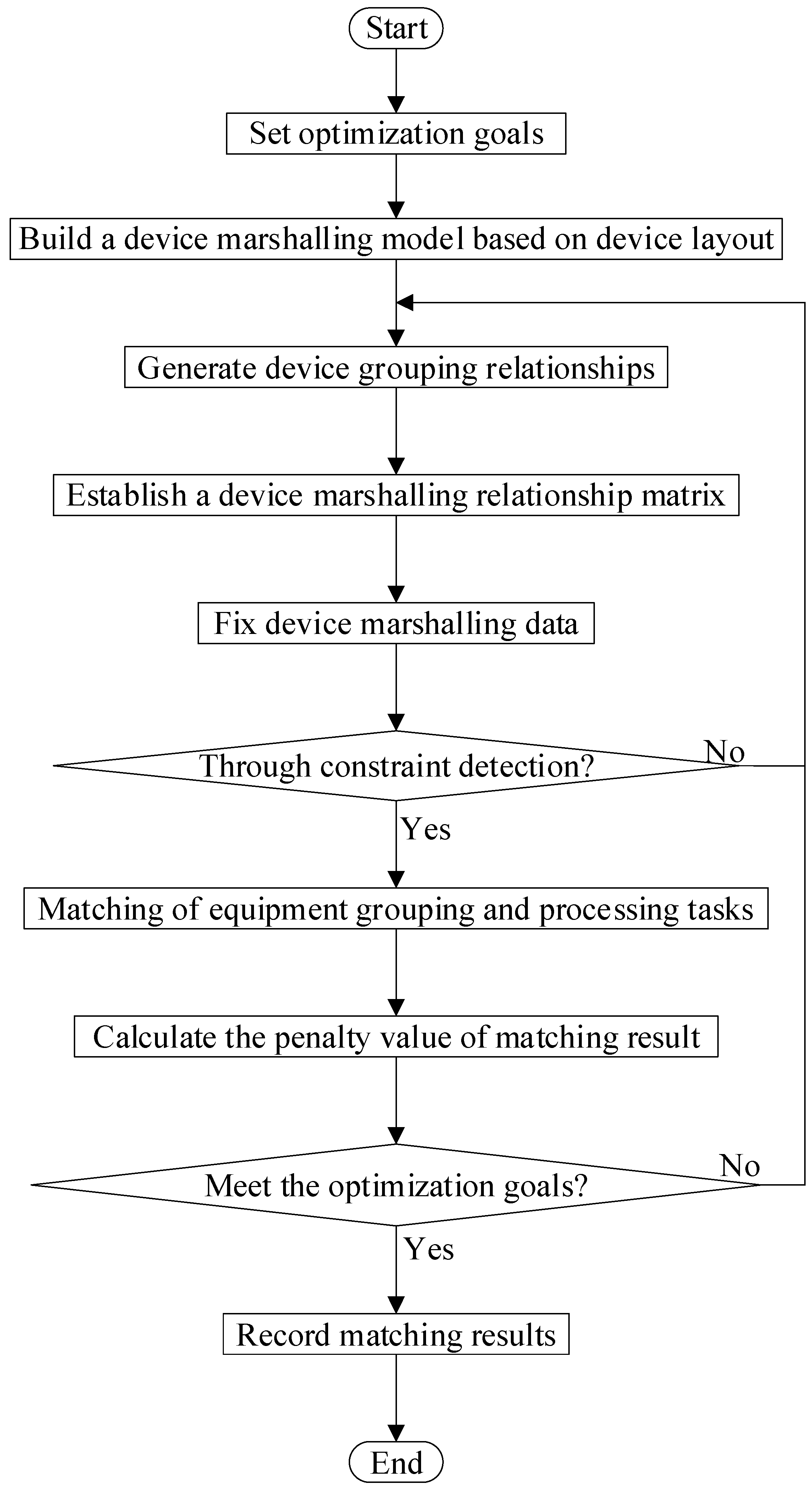
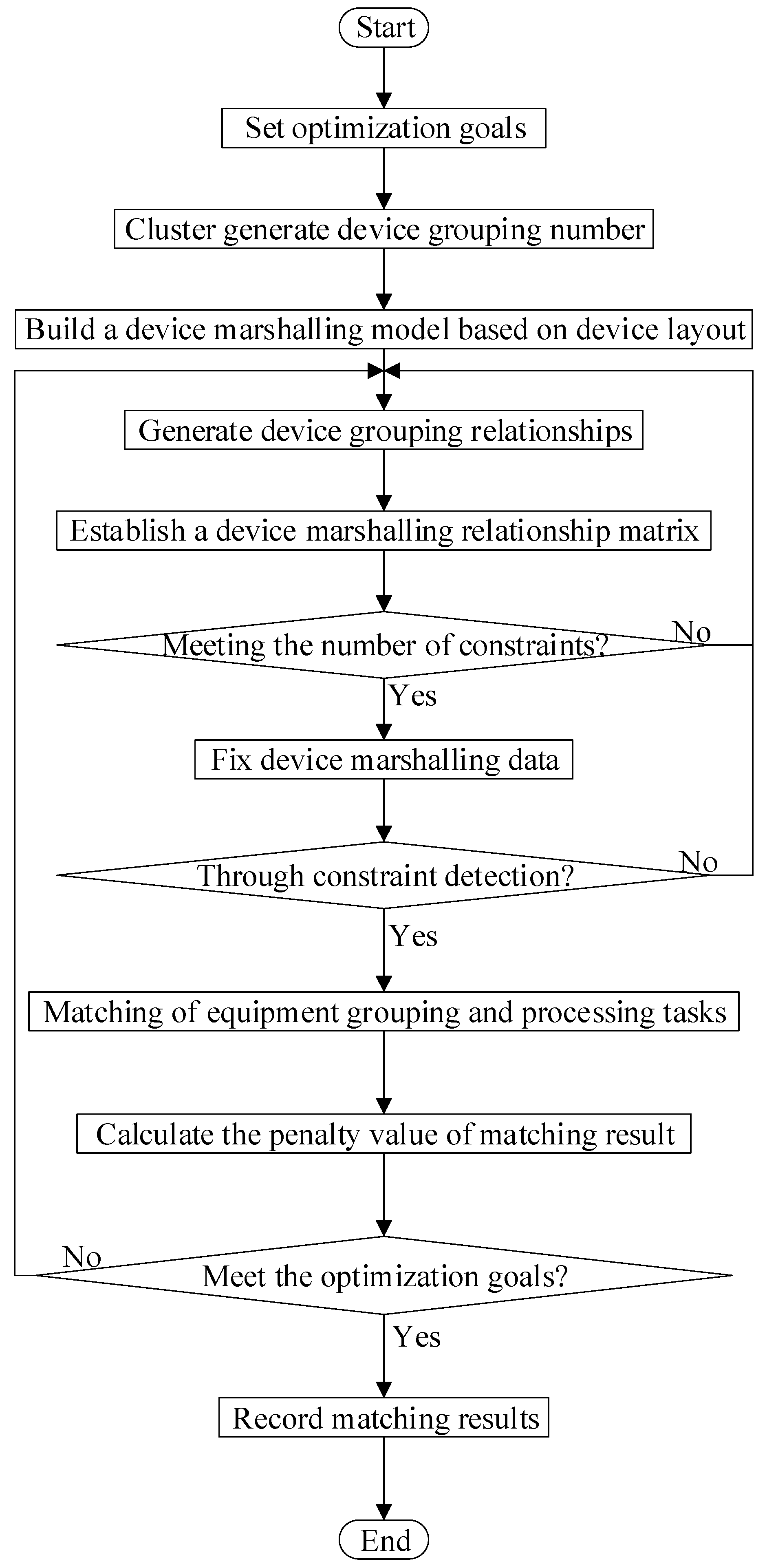
2.1. Equipment Marshalling Process

The flow of the bonding device grouping method based on the processing task [13] matching semiconductor package line is as shown in Figure 1 below:

Step 1: The minimum penalty value obtained by equipment grouping to provide capacity and processing task demand capacity matching is the optimization goal of equipment grouping.

Semiconductor manufacturing mainly consists of three phases: chip design, front wafer fabrication, and back-end packaging testing. The process of semiconductor package testing is dicing, loading, bonding, plastic sealing, deflashing, electroplating, printing, cutting, molding, visual inspection, finished product testing, packaging, and shipping. Semiconductor manufacturing is a dynamic and continuous process, so the time-limited cost of the bonding process segment cannot be derived separately. The utilization rate of the equipment can only be measured by considering the difference in the capacity of the equipment provided by the difference between the capacity provided and the capacity required.

Insufficient capacity is provided by the equipment group matching the processing task $W_P$.

$$P{C}_p=\max \left(0,g{w}_p-gm{a}_p\right)$$

(1)

Capacity redundancy is provided by the device group that matches the processing task $W_P$.

$$E{C}_p=\max \left(0,gm{a}_p-g{w}_p\right)$$

(2)

${gw}_p$ indicates the equipment capacity required for the processing task $p$. ${gma}_p$ indicates the processing capability of the equipment group matched by the processing task where $p$ can provide, $p\in \left\{1,2,L,PN\right\}$.

The punishment sum of equipment grouping and processing tasks.

$$f_o={\displaystyle \sum _{p=1}^{PN}\left({\alpha }_{p}P{C}_p+{\beta }_{p}E{C}_p\right)}$$

(3)

${\alpha }_p$ indicates the penalty for the capacity of the processing task $p$ ${\beta }_p$ indicates the redundancy penalty for capacity of the processing task $p$.

Step 2: Using graph theory to simplify the representation of a device as a node on a two-dimensional plane [14], abstracting all device points of this process into $n$ rows and $m$ columns of device matrices. $m_{i,j}$ represents a device of the $i-th$ row and the $j-th$ column.

$$M=\left[\begin{array}{cccc}{m}_{1,1}& m_{1,2}& k& m_{1,m}\\ m_{2,1}& m_{2,2}& k& m_{2,m}\\ m& m& m& m\\ m_{n,1}& m_{n,2}& k& m_{n,m}\end{array}\right]$$

(4)

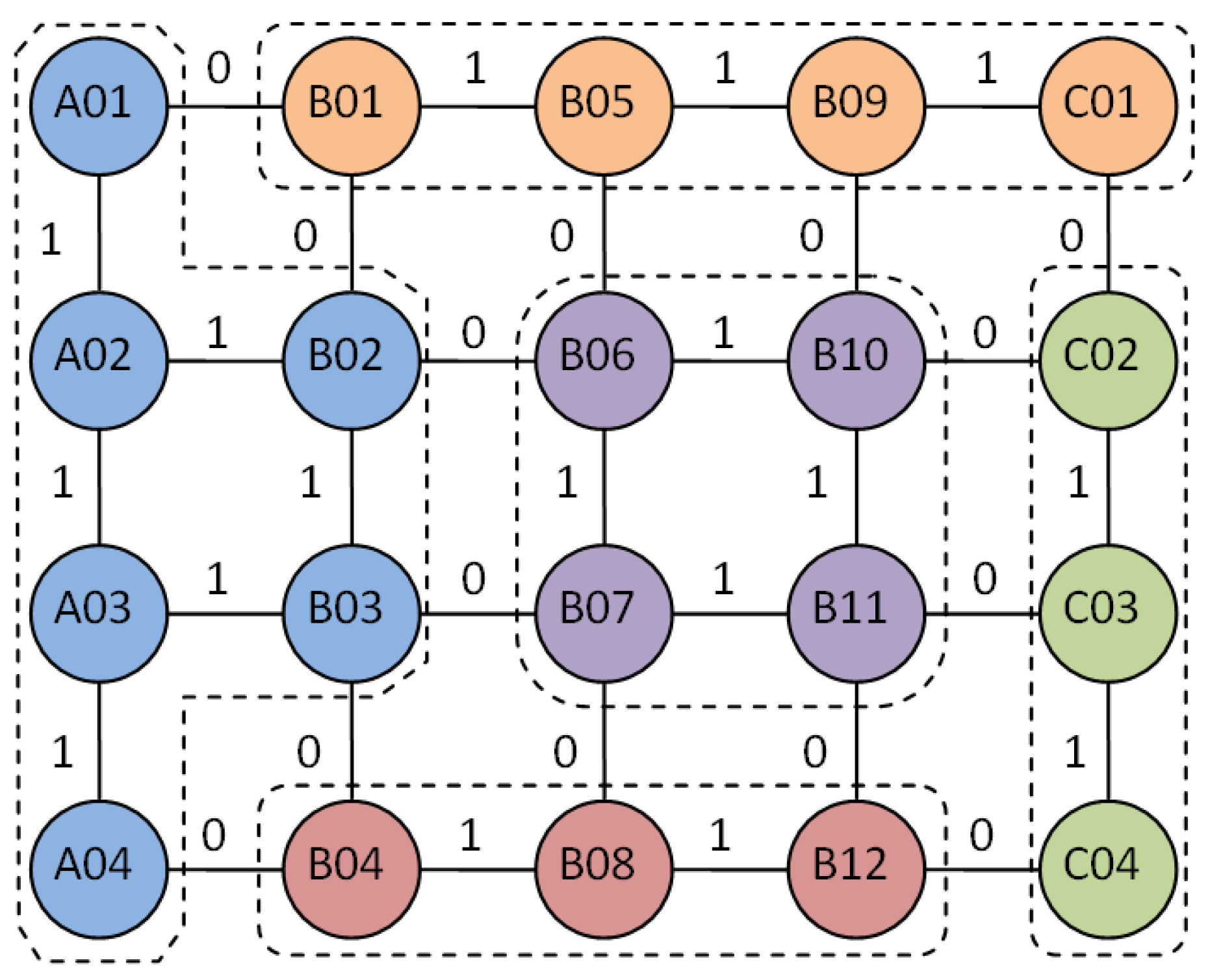
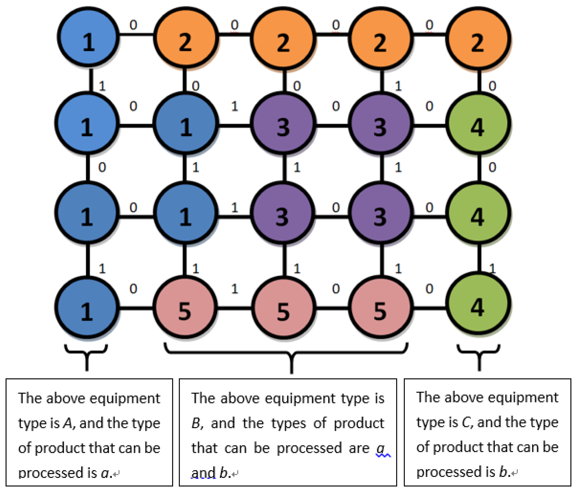
Step 3: All devices are connected by wires to form a network structure with device as node [15]. As shown in Figure 2, the association coefficient between the devices is randomly generated and represented by 0 and 1. The “0” indicates no association between the devices, i.e., the two devices are not in one group, and the “1” indicates the existence of an association, i.e., the two devices are edited in a group [16,17].

Step 4: According to the association coefficient between the devices, the device grouping row association matrix $LR$ and the column association matrix $LC$ are established by using the adjacency matrix, and the temporary device grouping $G$ is established.

The correlation matrix $LR$ between rows is as shown in Equation (5), and $l_{i,j}^r$ represents the row correlation coefficient between the $i-th$ row and the $i+1-th$ device of the $j-th$ column. When $l_{i,j}^r$ is “1”, it means that two adjacent devices are associated and can be grouped together. On the contrary, $l_{i,j}^r$ takes “0” to indicate no association. The correlation matrix $LC$ between the columns is as shown in Equation (6).

$$LR=\left[\begin{array}{cccc}{l}_{1,1}^r& l_{1,2}^r& l& l_{1,m}^r\\ l_{2,1}^r& l_{2,2}^r& l& l_{2,m}^r\\ m& m& l_{i,j}^r& m\\ l_{n-1,1}^r& l_{n-1,2}^r& l& l_{n-1,m}^r\end{array}\right]$$

(5)

$$LC=\left[\begin{array}{cccc}{l}_{1,1}^c& l_{1,2}^c& l& l_{1,m-1}^c\\ l_{2,1}^c& l_{2,2}^c& l& l_{2,m-1}^c\\ m& m& l_{i,j}^c& m\\ l_{n,1}^c& l_{n,2}^c& l& l_{n,m-1}^c\end{array}\right]$$

(6)

The associated device is grouped into a device group by the generated row and column association matrix. A temporary group number $g_t$ is assigned to indicate the group number of the $t-th$ device group. $GN$ represents the maximum group number for all groups.

Step 5: Correct the group association relationship. The temporary coding matrix of equipment grouping obtained in Step 4 may have a condition that conforms to the grouping rules but does not meet the actual grouping requirements. Therefore, it is necessary to correct the grouping relationship by employing the line scan and the column scan detection using the temporary group number $g_t$ of each group identification in Step 4.

Line detection starts from the 1st line and detects the nth line stop. It is necessary to check whether the correlation coefficient of each line is correct. According to the Equation (7), if the device group number $g_{i,j}$ of the $i-th$ row and the $j-th$ column is equal to the device group number $g_{i,j+1}$ of the $i-th$ row and the $j+1-th$ column, the device row association relationship $l_{i,j}^c$ is “1”. If it is “0”, it should be set to “1”.

$$l_{i,j}^c=\{\begin{array}{cc}0& M{g}_{i,j}\ne M{g}_{i+1,j}\\ 1& M{g}_{i,j}=M{g}_{i+1,j}\end{array}$$

(7)

Column detection starts from the 1st column and detects the $n-th$ column stop. It is necessary to check whether the correlation coefficient of each column is correct. According to the Equation (8), if the device group number $g_{i,j}$ of the $j-th$ column and the $i-th$ row is equal to the device group number $g_{i+1,j}$ of the $j-th$ column and the $i+1-th$ row, the device column association relationship $l_{i,j}^r$ is “1”. If it is “0”, it should be set to “1”.

$$l_{i,j}^r=\{\begin{array}{cc}0& M{g}_{i,j}\ne M{g}_{i,j+1}\\ 1& M{g}_{i,j}=M{g}_{i,j+1}\end{array}$$

(8)

Step 6: Closed position constraint refers to a device group or other device group that does not belong to this group is included in a two-dimensional plane. Such a completely enclosed relationship can be understood as a closed position. Constraint detection of device grouping. Constraint detection is divided into device group closed position relationship constraint detection and device type and processing type matching constraint detection. If any constraint detection fails, the grouping result is invalid, and the grouping step returns to Step 3.

(1) Constraint detection of closed position relationship by equipment grouping

The enclosed area formed by the grouping device cannot contain devices that do not belong to the device group, nor can it contain another independent device group. If such a grouping situation exists, the jurisdiction of the two equipment group managers overlaps, causing confusion in the production management organization.

To determine whether the device is completely in the closed range of the grouping, it is necessary to perform row detection and column detection according to the grouping relationship in the device grouping matrix $G$. If it is detected that a closed area formed in a device group contains devices that are not in this group, it is considered that the device grouping is unreasonable, and the temporary device grouping needs to be re-established. This inspection process needs to determine whether the grouping result is reasonable based on the results of the row and column test.

When the grouping information of the group to which the device of the $i-th$ row and the $j-th$ column belong is the same as the grouping number of the $t-th$ group, $g{z}_{t,i,j}$ is equal to “1”, otherwise it is equal to “0”. $F_{t,i}$ indicates whether the $i-th$ row of the $t-th$ device group contains devices that do not belong to the $t-th$ group. When the value is “1”, it means the device is not included, and when it is “0”, it means that it contains equipment that does not belong to the $t-th$ group.

$$F_{t,i}=\{\begin{array}{cc}1& {\displaystyle \sum _{j=m1t,i}^{m{2}_{t,i}}g{z}_{t,i,j}=\left(m{2}_{t,i}-m{1}_{t,i}\right)}\\ 0& {\displaystyle \sum _{j=m1t,i}^{m{2}_{t,i}}g{z}_{t,i,j}<\left(m{2}_{t,i}-m{1}_{t,i}\right)}\end{array}$$

(9)

$F_t^r$ indicates the result of row detection by the $t-th$ device group. The value of $F_t^r$ is “0”, indicating that the $t-th$ device group has detected that there are $non-t-th$ grouped devices in a certain device after the line detection. $F_t^c$ indicates the result of column detection by the $t-th$ device group. If $F_t^c$ is “0”, it indicates that the $t$ device group is detected by column and there is a $non-t$ group device in a column device.

$$F_t^r=\{\begin{array}{cc}1& \left({\displaystyle \sum _{i=n{1}_t}^{n{2}_t}{F}_{t,j}=n{2}_t-n{1}_t}\right)\cup \left(\left({\displaystyle \sum _{i=n{1}_t}^{n{2}_t}{F}_{t,j}<n{2}_t-n{1}_t}\right)\cap \left(\left(F_{t,n{1}_t}\ne 1\right)\cap \left(F_{t,n{2}_t}\ne 1\right)\right)\right)\\ 0& \left({\displaystyle \sum _{i=n{1}_t}^{n{2}_t}{F}_{t,j}<n{2}_t-n{1}_t}\right)\cap \left(F_{t,n{1}_t}=1\right)\cap \left(F_{t,n{2}_t}=1\right)\end{array}$$

(10)

$F_t$ indicates whether the closed area of the $t-th$ equipment group contains equipment that is not in this group. If $F_t$ is “0”, it indicates that the $F_t^r$ row detection result of the $t-th$ device group and the $F_t^c$ column detection result simultaneously determine the device having the $non-t-th$ group in the group.

$$F_t=\{\begin{array}{cc}1& F_t^r\ne 0\cup F_t^c\ne 0\\ 0& F_t^r=0\cap F_t^c=0\end{array}$$

(11)

$F$ indicates that the device grouping result satisfies the device location constraint. When all device groupings constitute a closed area, none of the non-grouped devices are included, and $F$ is equal to “1”.

$$F=\{\begin{array}{cc}1& {\displaystyle \sum _{t=1}^{GN}{F}_t=GN}\\ 0& {\displaystyle \sum _{t=1}^{GN}{F}_t<GN}\end{array}$$

(12)

(2) Constraint detection matching device type and processing type

The processed product type is represented by $k_x$, a total of $K_N$ product types. The device type is represented by $K_N$, which is a total of $KN$ device types. The relationship matrix $Kk$ whose product type matches the device type can be expressed as Equation (13). When $Kk{l}_{K_{y,}{k}_x}$ is “1”, the product type matches the device type. If it is “0”, the two do not match.

$$Kk=\left[\begin{array}{cccc}Kk{l}_{1,1}& Kk{l}_{1,2}& L& Kk{l}_{1,kn}\\ Kk{l}_{2,1}& Kk{l}_{2,2}& L& Kk{l}_{2,kn}\\ M& M& Kk{l}_{i,j}& M\\ Kk{l}_{KN,1}& Kk{l}_{KN,2}& L& Kk{l}_{KN,kn}\end{array}\right]$$

(13)

The matching relationship matrix $MK$ between the device and the device type is as shown in Equation (14). $MK{l}_{i,j,y}$ indicates the matching relationship between device type and device. $MK{l}_{i,j,y}$ equals “1” to indicate that the device matches the device type. If it is “0”, the device does not match the device type.

$$MK=\left[\begin{array}{cccc}M{kl}_{1,1,1}& M{kl}_{1,1,2}& L& M{kl}_{1,1,KN}\\ M{kl}_{1,2,1}& M{kl}_{1,2,2}& L& M{kl}_{1,2,KN}\\ M& M& Mk{l}_{i,j,y}& M\\ M{kl}_{n,m,1}& M{kl}_{n,m,2}& L& M{kl}_{n,m,KN}\end{array}\right]$$

(14)

$Mk$ indicates that the device and product type matching relationship matrix is as shown in Equation (15), which is obtained by multiplying the product of $MK$ and $Kk$.

$$Mk=\left[\begin{array}{cccc}M{kl}_{1,1,1}& M{kl}_{1,1,2}& L& M{kl}_{1,1,kn}\\ M{kl}_{1,2,1}& M{kl}_{1,2,2}& L& M{kl}_{1,2,kn}\\ M& M& Mk{l}_{i,j,x}& M\\ M{kl}_{n,m,1}& M{kl}_{n,m,2}& L& M{kl}_{n,m,kn}\end{array}\right]$$

(15)

For the device group $g_t$, the device set contained in the group is represented by $M{g}_t=\{M_{i,j}|g_{i,j}=g_t\}$. If $g_t$ and product type $k_x$ are grouped for any device, and $M{g}_t$ is included in $M{k}_x$ and $k_x$ belongs to $k$, the device grouping matches the device type and the processed product type matching constraint. If the constraint is not met, it is necessary to return to Step 3 to re-establish the correlation coefficient between the devices.

Step 7: Matching of equipment grouping and processing tasks

(1) Capacity provided by equipment grouping

The processing speed matrix $V$ is constructed according to the relationship matrix $Mk$ where the device matches the product type. $v_{i,j,x}$ is defined as the processing speed of the $k_x$ type product by the device in the $i-th$ row and the $j-th$ column.

$$V_{{i,j,k}_x}=\{\begin{array}{cc}{v}_{i,j,k_x}& Mk{l}_{i,j,k_x}=1\\ 0& Mk{l}_{i,j,k_x}=0\end{array}$$

(16)

$$V=\left[\begin{array}{cccc}{v}_{1,1,k_1}& v_{1,2,k_2}& l& v_{1,m,k_{kn}}\\ v_{1,2,k_1}& v_{1,2,k_2}& l& v_{1,2,k_{kn}}\\ m& m& v_{i,j,k_x}& m\\ v_{n,m,k_1}& v_{n,m,k_2}& l& v_{n,m,k_{kn}}\end{array}\right]$$

(17)

A matrix is constructed based on product type to provide capacity matrix $Gga$, where $g{a}_{t,k_x}$ indicates that the equipment group $g_t$ produces the processing capacity of the $k_x$ type product, ${ga}_{t,k_x}=\left({\displaystyle \sum _{i=n{1}_t}^{n{2}_t}{\displaystyle \sum _{j=m{1}_t}^{m{2}_t}{V}_{i,j,k_x}}}\right)gT,i\in \left\{n{1}_t,\dots ,n{2}_t\right\},j\in \left\{m{1}_t,\dots ,m{2}_t\right\}$.

$$Gga=\left[\begin{array}{cccc}g{a}_{1,k_1}& g{a}_{1,k_2}& l& g{a}_{1,k_{kn}}\\ g{a}_{2,k_2}& g{a}_{2,k_2}& l& g{a}_{2,k_{kn}}\\ m& m& g{a}_{t,k_x}& m\\ g{a}_{GN,k_1}& g{a}_{GN,k_2}& l& g{a}_{GN,k_{kn}}\end{array}\right]$$

(18)

(2) Demand capacity of processing tasks

The processing task set is represented by $W_p$,$W_p=\left\{W_p|p\in \left\{1,2,\dots ,PN\right\}\right\}$.$W_p$ represents the $p-th$ processing task, the product type of the $p-th$ processing task is represented by $K_p$, and the product type set constituting the processing task is represented by $KP$, $KP=\left\{K_p|p\in \left\{1,2,\dots ,PN\right\}\right\}$. The set of processing tasks for product type $k_x$ is represented by $W{P}_x$,$W{P}_x=\left\{W_p|k_x=k_p,p\in \left\{1,2,\dots ,PN\right\}\right\}$, and $W{P}_x\subseteq WP$, ${gw}_p$ indicates the demand capacity of the $p-th$ processing task, and the processing task demand capacity set is represented by $GW$,$GW=\left\{{gw}_p|p\in \left\{1,2,\dots ,PN\right\}\right\}$.

(3) Equipment grouping matching the processing task

The total number of production equipment marshalling $GN$ should be greater than or equal to the total number of tasks to be assigned $PN$. The number of selectable device groups corresponding to the product type $k_x$ should be greater than or equal to the number of tasks in the processing task set whose product type is $k_x$.

The matrix matching the processing task demand ability and the equipment group capability is represented by $Gamc$. $Gamc=\left\{\left\{\langle {gw}_p,gm{a}_p\rangle |p\in \left\{1,2,\dots ,PN\right\}\right\}\right\}$.$gm{a}_p$ indicates the processing capacity of the equipment group, ${gw}_p$ indicates the demand capacity of the processing task. The $PN$ processing tasks are assigned to the equipment group. It is necessary to sort the processing task $W_p$ according to the descending order of the required task capacity $GW$. Then it is necessary to obtain the sorted device task collection queue $W_{p^{\prime }}$ and the product type sequence $k_{p^{\prime }}$ corresponding to $W_{p^{\prime }}$.

According to the relationship matrix $Mk$ matched by the device and the product type, the device group capable of processing the product is selected by the product type of the processing task, and the matching relationship matrix $Gk$ of the device grouping and the product type are constructed.

$$Gk=\left[\begin{array}{cccc}gk{l}_{1,k_1}a{s}_1& gk{l}_{1,k_2}a{s}_1& L& gk{l}_{1,k_{kn}}a{s}_1\\ gk{l}_{2,k_1}a{s}_2& gk{l}_{2,k_2}a{s}_2& L& gk{l}_{2,k_{kn}}a{s}_2\\ M& M& gk{l}_{t,k_x}a{s}_t& M\\ gk{l}_{GN,k_1}a{s}_{GN}& gk{l}_{GN,k_2}a{s}_{GN}& L& gk{l}_{GN,k_{kn}}a{s}_{GN}\end{array}\right]$$

(19)

The element ${gkl}_{t,x}$ in the matrix $Gk$ indicates the matching relationship between product type and device grouping. Its value of “1” means that the device group $g_t$ contains the device that satisfies the matching relationship between the device type and the product type.

When the device group is not assigned a task in the initial state, all ${as}_t$ is 1. The processing product type is $k_{p^{\prime }}$ and processing task is $W_{p^{\prime }}$. Selected device grouping is set as $G{g}_{k_{p^{\prime }}}$, and each device group is calculated in $G{g}_{k_{p^{\prime }}}$. The processing capacity and the established $G{g}_{k_{p^{\prime }}}$ corresponds to the equipment group capacity set $G{ga}_{k_{p^{\prime }}}$,$G{ga}_{k_{p^{\prime }}}=\left\{g{a}_{t,k_x}|gk{l}_{t,k_x}=1,a{s}_t=1,k_x=k_{p^{\prime }},t\in \left\{1,2,\dots ,PN\right\}\right\}$. $g{a}_{t,k_x}$ is the processing capability of equipment group $g_t$ to produce $k_x$ type products. When $G{g}_{k_{p^{\prime }}}$ is not an empty set, the processing task $W_{p^{\prime }}$ should be assigned to $G{ga}_{k_{p^{\prime }}}$. The device group with the largest processing capability in the set is represented by $gm{a}_{p^{\prime }}$,${gma}_{p^{\prime }}=\left\{g{a}_{q,k_{p^{\prime }}}|q=\min \left\{t|\max \left(Gg{a}_{k_{p^{\prime }}}\right)\right\}\right\}$. The task $W_{p^{\prime }}$ is matched to the device group $g_q$, where $q=\min \left\{t|\max \left(Gg{a}_{k_{p^{\prime }}}\right)\right\}$, and the row corresponding to the $g_q$ in the matrix corresponds to ${as}_q=0$, indicating that the device group was assigned tasks. When the next task matches, the device group no longer participates in the matching of devices and tasks. After all the processing tasks are matched, the device group capability matching set $Gam{c}^{\prime }$ and the device group matching set $Gm{c}^{\prime }$ are matched with $G{W}^{\prime }$ and $W_{p^{\prime }}$. Then, according to the order of the original processing task $WP$ the equipment group matching set $Gmc$ matching the order of the processing tasks is obtained, $Gmc=\left\{\langle W_{p^{\prime }},g_{q^{\prime }}\rangle |p\in \left\{12,\dots ,PN\right\},q^{\prime }\in \left\{1,2,\dots ,GN\right\}\right\}$. The processing task requirement capability and the device group capability matching set $Gamc$ corresponding to the device group matching set $Gmc$ are obtained.

Step 8: The optimization goal of device grouping is the penalty value $f_o$ minimum for device grouping and processing tasks. If the optimization range is satisfied, the temporary grouping result is saved. If the requirement is not met, the process returns to Step 3 until the maximum number of iterations is reached, and the grouping corresponding to the minimum penalty value is stopped as the final grouping result.

2.2. Analysis of Equipment Grouping Methods Based on Processing Task Matching

Compared with the prior art, the grouping method has the following advantages:

(1) The concept of directed graph in graph theory is used to abstract the device set into a matrix, and to establish a device marshalling model, and change the adjacency matrix to change the relationship between devices.

(2) The situation of the device fixed grouping of the bonding process segment is changed, and the device can be dynamically grouped according to the released production task. In the process of grouping equipment, the equipment in the group is in a complete unicom area, which is convenient for the staff of the production line.

(3) The evaluation index of the capacity matching between the capacity provided by the equipment group and the processing task is established to better meet the purpose of matching the equipment grouping and processing tasks, and to ensure the rationality of the dynamic grouping results.

However, the proposed bonding device grouping method based on processing task matching semiconductor packaging lines is not without defects. For example, when the correlation matrix is generated. Since the correlation coefficient is 0 and 1 randomly generated by the rand function, the association relationship between the devices is random, and the devices that can be associated together and grouped together are also randomly combined. The randomness generated by the correlation coefficient may cause the generated temporary grouping number to be too large or too small, thus generating a grouping deviation. The grouping deviation refers to the absolute value of the difference between the number of groups obtained by the equipment grouping and the number of processing tasks. Too many groups may lead to devices with no processing tasks to match, thus wasting processing power. If the number of groups is too small or even smaller than the number of processing tasks, the grouping cannot be matched with the processing and production tasks. Considering that the production equipment itself has many characteristics, it can be clustered according to certain dimensions. Therefore, the density peak-based clustering method (CFSFDP) with better effect in unsupervised learning has been improved. In the paper, I made a modification and made a detailed explanation of the device grouping method improved by adding the CFSFDP algorithm. Therefore, based on the proposed grouping method, the CFSFDP algorithm is added to the divergence of the number of groups $GN$, and the reasonable range of the number of device groupings is obtained according to the attribute information of the device clustering. Attribute information refers to the self-contained attributes such as processing speed, device type, device location, and device parameters for different types of products.

3. Grouping Method of Semiconductor Bonding Equipment Based on CFSFDP Algorithm for Dynamic Matching According to Processing Tasks

Clustering is called unsupervised learning in the field of machine learning and pattern recognition. In the absence of prior knowledge, clustering classifies data according to the similarity between data objects. Usually, the similarity between data objects is the distance between data objects is determined. The CFSFDP clustering algorithm is based on the idea of density clustering. The implementation process is simple. Only the data object distance is calculated in the algorithm processing process, which greatly reduces the computational cost of the algorithm. The algorithm only has one parameter and does not require iteration. This algorithm is used to improve the device grouping method. Starting from the grouping deviation that has the greatest impact on the equipment grouping result, the effective range of the number of groupings is used to reduce the invalid grouping result and reduce the grouping deviation.

3.1. Overview of CFSFDP Clustering Algorithm

The CFSFDP algorithm [18,19] is a clustering algorithm based on density peaks. The premise fora this clustering approach is mainly based on two assumptions: first, compared with other data points, the local density of the cluster center point is larger. Second, the distance between the cluster center and other points with higher local density is greater. The cluster center selected by the CFSFDP algorithm has a very large density, and the distance between different cluster centers is very far. This selection rule is consistent with the actual law. In the process of processing a large number of data sets, the superiority and simplicity of the algorithm are reflected.

For any data point $x_i$, the data point local density ${\rho }_i$ and the point distance ${\delta }_i$ are defined. The local density ${\rho }_i$ represents the number of data points in the data set $S$ that is less than $d_c$ from the data point $x_i$. The adjacent density point distance ${\delta }_i$ represents the minimum distance between the point where the local density is greater than the local density of the data point $x_i$ and the $x_i$ point in the data set $S={\left\{x_i\right\}}_{i=1}^N$. For any point $x_i$ in the data set $S={\left\{x_i\right\}}_{i=1}^N$, there exists $\left({\rho }_i,{\delta }_i\right)$, and a plane rectangular coordinate system is established, the abscissa is $\rho$, and the ordinate is $\delta$. The $\left({\rho }_i,{\delta }_i\right)$ corresponding to each data point $x_i$ in the data set is drawn in the established plane rectangular coordinate system, and the clustering decision diagram of the data set is established. The description of the cluster center by the CFSFDP algorithm is available, and data points with large $\rho$ and $\delta$ in the data set may become cluster centers.

3.2. Application of CFSFDP Clustering Algorithm in Equipment Marshalling Process

The attribute information of all devices are collected in a certain area of the bonding process segment, and the continuous attributes to create a new multi-dimensional data set are selected, and the CFSFDP algorithm is used to cluster the data sets. After clustering, several clusters are automatically generated. The number of classes can provide a constraint range for the number of $GN$s generated in the device grouping process, and reduce the grouping bias. Figure 3 shows improved device grouping flow chart.

Through the CFSFDP algorithm, the devices in the bonding process are automatically clustered, and the maximum number of clusters $GN$ is generated by the number of clusters generated by the clustering result. Taking a small-scale device group as an example, a 4 × 5 device group is selected, and the collection device information is organized into an input data set. The CFSFDP algorithm reads the information of each device and numbers them according to the input order, and saves the attribute information of multiple dimensions. The Euclidean distance between the devices in all bonding process segments is then calculated and a similarity matrix is formed. The parameter $d_c$ is determined according to the number of data points of the data set, and the local density ${\rho }_i$ of each data point and the relative density point distance ${\delta }_i$ are calculated. ${\gamma }_i$ is a value obtained by multiplying the local density ${\rho }_i$ corresponding to all data points by its corresponding relative density point distance ${\delta }_i$, and then grading the ${\gamma }_i$ in descending order. Then, through the principle of decision graph, several data points with relatively large local density $\rho$ and relative density point distance $\delta$ are selected as the cluster center of clusters [18]. A reasonable range of the number of groups of these devices is obtained, and used as a condition to judge whether the temporary grouping is reasonable and effective.

As shown in the decision diagram of Figure 4 below, the local density $\rho$ is the coordinate axis $x$, and the relative density point distance $\delta$ is the coordinate axis $y$. The local density ${\rho }_i$ and relative density point distance ${\delta }_i$ of these 20 devices are represented in the decision graph. The cluster center selected according to the CFSFDP algorithm is based on the principle that the density of the data points is very large and the distance between different cluster centers is very far. From 20 data points, a data point having a large local density compared with other data points and a large distance from other points with higher local density is found as the cluster center point of the 20-device data. According to Figure 4, the selected data points 6, 7, 10, 11, 12, 14, and 15 are points at which the local density ${\rho }_i$ and the relative density point distance ${\delta }_i$ are simultaneously large. The product ${\gamma }_i$ of the local density ${\rho }_i$ corresponding to the 20 data points and the relative density point distance ${\delta }_i$ are arranged in descending order shown in Figure 5. In the screening of cluster centers, it mainly depends on two important parameters, local density $\rho$ and distance δ of adjacent density points. The larger the product of the two, the more likely it is to become the center of the cluster. The product’s product is obtained in descending order, and it can be seen that the falling slope has a distinct “inflection point”. According to the cluster center map, the three points of 4, 6, and 11 have made significant changes in both the slope and the cluster center weight. For the cluster center, the weight of the cluster center has a very small number and the value is obviously large. As the weight of the cluster center decreases, the weight of the cluster center becomes slower and the value becomes smaller. The weight of the cluster center in the non-cluster has a large number, the value is obviously small and the difference between the points is small. Therefore, these three points may belong to the cluster center. Then, the average value α is obtained for the cluster center weight $\gamma$ of all points, and the ${\gamma }_i$ corresponding to each data point is compared with $\alpha$. When ${\gamma }_i$ is greater than $\alpha$, the corresponding data points are used as the cluster center. The cluster center weight $\gamma$ of point 4 is lower than the average value α, so it is excluded as the cluster center. The number of cluster clusters obtained is taken as the maximum number of device groups [20].

After the temporary device group $G$ is created, it is necessary to determine whether the number of groups conforms to the maximum number of groups generated by the CFSFDP algorithm and the number of groups formed by the number of work tasks. If the grouping range requirements are met, the steps to modify the grouping data are performed. If they are not met, the relationship matrix is regenerated.

The simplified steps of the device grouping method improved by adding the CFSFDP algorithm are as follows.

Step 1: The minimum penalty value obtained by equipment grouping to provide capacity and processing task demand capacity matching is the optimization goal of equipment grouping.

The punishment sum of equipment grouping and processing tasks.

$$f_o={\displaystyle \sum _{p=1}^{PN}\left({\alpha }_{p}P{C}_p+{\beta }_{p}E{C}_p\right)}$$

(20)

${\alpha }_p$ indicates the penalty for the capacity of the processing task $p$. ${\beta }_p$ indicates the redundancy penalty for capacity of the processing task $p$.

Step 2: Using graph theory to simplify the representation of a device as a node on a two-dimensional plane [14], abstracting all device points of this process into $n$ rows and $m$ columns of device matrices. $m_{i,j}$ represents a device of the $i-th$ row and the $j-th$ column.

$$M=\left[\begin{array}{cccc}{m}_{1,1}& m_{1,2}& k& m_{1,m}\\ m_{2,1}& m_{2,2}& k& m_{2,m}\\ m& m& m& m\\ m_{n,1}& m_{n,2}& k& m_{n,m}\end{array}\right]$$

(21)

Step 3: The collection device information is organized into an input data set, and the CFSFDP algorithm reads the information of each device and numbers them in the input order. The Euclidean distance between the devices in all bonding process segments is then calculated and a similarity matrix is formed. The parameter $d_c$ is determined according to the number of data points of the data set, and the local density ${\rho }_i$ of each data point and the relative density point distance ${\delta }_i$ are calculated, and the product ${\gamma }_i$ of the local density ${\rho }_i$ corresponding to all data points and the relative density point distance ${\delta }_i$ is descended. Then, through the principle of decision graph, several data points with relatively large local density $\rho$ and relative density point distance $\delta$ are selected as the cluster center of the cluster, and then the reasonable number of groups of these devices is obtained.

Step 4: All devices are connected by wires to form a network structure with device as node. The association coefficient between the devices is randomly generated and represented by 0 and 1. The “0” indicates no association between the devices, i.e., the two devices are not in one group, and the “1” indicates the existence of an association, i.e., the two devices are edited in a group.

Step 5: According to the association coefficient between the devices, the device grouping row association matrix $LR$ and the column association matrix $LC$ are established by using the adjacency matrix, and the temporary device grouping $G$ is established.

$$LR=\left[\begin{array}{cccc}{l}_{1,1}^r& l_{1,2}^r& l& l_{1,m}^r\\ l_{2,1}^r& l_{2,2}^r& l& l_{2,m}^r\\ m& m& l_{i,j}^r& m\\ l_{n-1,1}^r& l_{n-1,2}^r& l& l_{n-1,m}^r\end{array}\right]$$

(22)

$$LC=\left[\begin{array}{cccc}{l}_{1,1}^c& l_{1,2}^c& l& l_{1,m-1}^c\\ l_{2,1}^c& l_{2,2}^c& l& l_{2,m-1}^c\\ m& m& l_{i,j}^c& m\\ l_{n,1}^c& l_{n,2}^c& l& l_{n,m-1}^c\end{array}\right]$$

(23)

The associated device is grouped into a device group by the generated row and column association matrix. A temporary group number $g_t$ is assigned to indicate the group number of the $t-th$ device group. $GN$ represents the maximum group number for all groups.

Step 6: It is determined whether the temporary device grouping number GN is within the effective grouping number composed of the maximum number of groupings obtained by clustering and the number of processing tasks. If the thief continues to step 7 within this range, otherwise return to step 4 to re-establish the association.

Step 7: Correct the group association relationship. The temporary coding matrix of equipment grouping obtained in Step 5 may have a condition that conforms to the grouping rules but does not meet the actual grouping requirements. Therefore, it is necessary to correct the grouping relationship by employing the line scan and the column scan detection using the temporary group number $g_t$ of each group identification in Step 5.

$$l_{i,j}^c=\{\begin{array}{cc}0& M{g}_{i,j}\ne M{g}_{i+1,j}\\ 1& M{g}_{i,j}=M{g}_{i+1,j}\end{array}$$

(24)

$$l_{i,j}^r=\{\begin{array}{cc}0& M{g}_{i,j}\ne M{g}_{i,j+1}\\ 1& M{g}_{i,j}=M{g}_{i,j+1}\end{array}$$

(25)

Step 8: Closed position constraint refers to a device group or other device group that does not belong to this group is included in a two-dimensional plane. Such a completely enclosed relationship can be understood as a closed position. Constraint detection of device grouping. Constraint detection is divided into device group closed position relationship constraint detection and device type and processing type matching constraint detection. If any constraint detection fails, the grouping result is invalid, and the grouping step returns to Step 4. Constraint detection of closed position relationship by equipment grouping.

Step 9: Matching of equipment grouping and processing tasks

(1) Capacity provided by equipment grouping

A matrix is constructed based on product type to provide capacity matrix $Gga$, where $g{a}_{t,k_x}$ indicates that the equipment group $g_t$ produces the processing capacity of the $k_x$ type product, ${ga}_{t,k_x}=\left({\displaystyle \sum _{i=n{1}_t}^{n{2}_t}{\displaystyle \sum _{j=m{1}_t}^{m{2}_t}{V}_{i,j,k_x}}}\right)gT,i\in \left\{n{1}_t,\dots ,n{2}_t\right\},j\in \left\{m{1}_t,\dots ,m{2}_t\right\}$.

$$Gga=\left[\begin{array}{cccc}g{a}_{1,k_1}& g{a}_{1,k_2}& l& g{a}_{1,k_{kn}}\\ g{a}_{2,k_2}& g{a}_{2,k_2}& l& g{a}_{2,k_{kn}}\\ m& m& g{a}_{t,k_x}& m\\ g{a}_{GN,k_1}& g{a}_{GN,k_2}& l& g{a}_{GN,k_{kn}}\end{array}\right]$$

(26)

(2) Demand capacity of processing tasks

The processing task set is represented by $W_p$,$W_p=\left\{W_p|p\in \left\{1,2,\dots ,PN\right\}\right\}$.$W_p$ represents the $p-th$ processing task, the product type of the $p-th$ processing task is represented by $K_p$, and the product type set constituting the processing task is represented by $KP$, $KP=\left\{K_p|p\in \left\{1,2,\dots PN\right\}\right\}$. The set of processing tasks for product type $k_x$ is represented by $W{P}_x$,$W{P}_x=\left\{W_p|k_x=k_p,p\in \left\{1,2,\dots ,PN\right\}\right\}$, and $W{P}_x\subseteq WP$, ${gw}_p$ indicates the demand capacity of the $p-th$ processing task, and the processing task demand capacity set is represented by $GW$,$GW=\left\{{gw}_p|p\in \left\{1,2,\dots PN\right\}\right\}$.

(3) Equipment grouping matching the processing task

The total number of production equipment marshalling $GN$ should be greater than or equal to the total number of tasks to be assigned $PN$. The number of selectable device groups corresponding to the product type $k_x$ should be greater than or equal to the number of tasks in the processing task set whose product type is $k_x$.

The matrix matching the processing task demand ability and the equipment group capability is represented by $Gamc$. $Gamc=\left\{\left\{\langle {gw}_p,gm{a}_p\rangle |p\in \left\{1,2,\dots ,PN\right\}\right\}\right\}$.$gm{a}_p$ indicates the processing capacity of the equipment group, ${gw}_p$ indicates the demand capacity of the processing task.

Step 10: The optimization goal of device grouping is the penalty value $f_o$ minimum for device grouping and processing tasks. If the optimization range is satisfied, the temporary grouping result is saved. If the requirement is not met, the process returns to Step 3 until the maximum number of iterations is reached, and the grouping corresponding to the minimum penalty value is stopped as the final grouping result.

4. Simulation Verification and Results Analysis

4.1. Simulation Experiment Design Related Information

The simulation experiment is divided into the comparison of the equipment grouping methods before and after the application of the processing task matching under different equipment scales, and the comparison of the equipment grouping methods before and after the application of the processing task matching with different discrete degree requirements. For the simulation experiment, we used MATLAB R2016a platform, with the following hardware parameters: CPU R 2.50 dual core and 4G memory.

The semiconductor industry is a dynamic production process, and there are many process segments. The bonding is only one process segment of the package test part, and the equipment of the bonding process segment is divided into multiple regions. This article only selects the equipment of a certain region. In the simulation experiment, the equipment was divided into three types: $A$, $B$, and $C$. The processing task product types were divided into two types: $a$ and $b$. Type $a$ products could only be processed by type $A$, and type $B$ equipment, and type $b$ products could only be processed by type $B$ and type $C$ equipment. The device grouping scale was divided into five types: 3 × 4 device group, 4 × 5 device group, 7 × 7 device group, 10 × 10 device group, and 15 × 15 device group.

Demand capacity was divided into dense and discrete according to the size of the difference coefficient [21]. The difference coefficient is the relative difference quantity, which can be used to compare the differences between data units, and can also be used to compare the differences of similar phenomena at different levels. The most commonly used coefficient of variation is proposed by Pearson (K.). The coefficient of variation removes the average standard deviation and multiplies it by 100% to form a percentage. The simulation experiment is carried out by selecting the demand capacity set of five different difference coefficients. The calculation formula is as follows, where $S$ is the standard deviation and $M$ is the average.

$$CV=\frac{S}{M}\times 100\%$$

(27)

4.2. Definition of Evaluation Indicators

The production grouping deviation $d$ is the difference between the number of equipment groupings $GN$ and the number of processing tasks $PN$.

$$d=GN-PN$$

(28)

Since the production line requires that the product type that can be processed in the equipment group is the same as that of the processing task, and the equipment constructed by the grouping equipment cannot contain equipment or equipment groups that are not grouped, the resulting grouping result may not be detected by the constraint. The proportion of detection by constraint m indicates the ratio of the generated grouping result by the constraint detection, $GN$ indicates the number of generating device grouping groups, and $F_g$ indicates the number of grouping groups that have not passed the constraint detection.

$$r=\frac{GN-F_g}{GN}\times 100\%$$

(29)

In actual production, production capacity redundancy can speed up production, but it can also lead to the waste of resources, and insufficient capacity allocation that can cause production delays. The optimal equipment grouping result is obtained when the penalty value for equipment grouping and processing tasks is the smallest. The device grouping and processing task penalty function is as follows [22].

$$f_o={\displaystyle \sum _{p=1}^{PN}\left({\alpha }_{p}P{C}_p+{\beta }_{p}E{C}_p\right)}$$

(30)

In the formula, ${\alpha }_p$ indicates the penalty for the capacity of the processing task $p$. ${\beta }_p$ indicates the redundancy penalty for capacity of the processing task $p$.

4.3. Analysis of Experimental Results

In

Table 1. Comparison of pre-improvement equipment methods and improved equipment methods under different equipment scales when demand capacity distribution is intensive.

Equipment Scale	Distance Parameter $d_c$	Device Grouping Method Based on Processing Task Matching			Machining Task Matching Semiconductor Bonding Device Grouping Method Based on CFSFDP Algorithm
		$f_o$	$d$	$r$	$f_o$	$d$	$r$
3 × 4	0.20	113.15	1.60	89.90	108.52	0	90.20
4 × 5	0.40	113.35	2.10	80.80	106.84	1.40	83.80
7 × 7	0.63	139.21	9.42	97.70	120.69	6.84	97.30
10 × 10	1.16	256.92	22.10	92.30	123.79	11.61	95.00
15 × 15	2.93	303.39	52.30	93.90	307.30	50.50	94.80

,

Table 2. Comparison of pre-improvement equipment methods and improved equipment methods under different equipment scales when demand capacity distribution is discrete.

Equipment Scale	Distance Parameter $d_c$	Device Grouping Method Based on Processing Task Matching			Machining Task Matching Semiconductor Bonding Device Grouping Method Based on CFSFDP Algorithm
		$f_o$	$d$	$r$	$f_o$	$d$	$r$
3 × 4	0.20	134.82	1.50	77.00	133.92	0	78.70
4 × 5	0.40	89.17	1.30	88.50	87.03	1.02	91.10
7 × 7	0.63	154.31	9.59	96.40	106.20	6.80	98.40
10 × 10	1.16	258.46	22.3	92.50	110.502	11.52	94.80
15 × 15	2.93	282.82	52.23	95.90	273.852	44.80	94.20

and

Table 3. Comparison of pre-improvement equipment methods and improved equipment methods for different discrete-degree demand capacity.

Demand Capacity	Difference Coefficient $CV$	Device Grouping Method Based on Processing Task Matching			Machining Task Matching Semiconductor Bonding Device Grouping Method Based on CFSFDP Algorithm
		fo	$d$	$r$	$f_o$	$d$	$r$
GW1	0.09	102.24	0.93	74.00	101.59	0.64	76.50
GW2	0.11	115.04	1.03	83.30	108.94	0.63	86.82
GW3	0.28	114.06	0.86	84.51	112.77	0.55	87.40
GW4	0.39	112.04	0.95	83.10	108.13	0.71	85.70
GW5	0.47	114.14	0.97	80.35	112.79	0.65	85.00

, method one represents semiconductor bonding device grouping method based on dynamic matching of processing task, method two represents method for grouping semiconductor bonding equipment based on CFSFDP algorithm for dynamic matching of processing tasks.

Table 1 shows the experimental results of grouping equipment groups with different equipment scales based on the processing of job matching and the processing of the semiconductor bonding equipment based on the CFSFDP algorithm. Table 2 shows the experimental results of grouping device groups based on different device sizes when the internal data distribution of the demand capacity set is discrete. The experimental results show that under the demand capacity set with the same difference coefficient, the equipment scale remains unchanged, and the evaluation index of the semiconductor bonding equipment grouping method based on CFSFDP algorithm is better than the equipment grouping method before the improvement. Table 1 shows that after adding the CFSFDP algorithm, the grouping deviation $d$ is reduced by about 24.4% on average, while from the Table 2 it can be seen that the grouping deviation $d$ is reduced by about 35.6% on average. Before the device is grouped, the cluster of the device based on the density peak is obtained, as well as the cluster number of the device set. The maximum number of the device groups is obtained, thereby generating a reasonable range of device grouping. Therefore, the grouping deviation is reduced without changing the number of processing tasks. It can be seen from Table 1 that the coincidence rate $r$ was increased by 1.3%, and the coincidence rate $r$ in Table 2 was increased by 1.7% on average. The CFSFDP algorithm aggregates similar devices into one class, and reduces unreasonable grouping results. This increases the proportion of devices that are constrained by the closed area constraints and the matching of the equipment to the processed product type. The optimization goal of equipment grouping is to obtain the lowest penalty value for the equipment grouping and processing tasks. As is shown in Table 1, the equipment grouping and processing task penalty and the value $f_o$ were reduced by 24.6% on average, and the $f_o$ in Table 2 was reduced by 22.6% on average. This shows that the difference between the capacity of the device group and the capacity required for the processing task is reduced after adding the CFSFDP algorithm and improving the processing task sequence. Moreover, the value of $P{C}_p$ and $E{C}_p$ are reduced, and equipment marshalling and processing tasks are better matched.

Comprehensive analysis of the data shown in Table 1 and Table 2, reveal that under the same device grouping method, the size of the device may have a certain impact on the device grouping results. As shown in Figure 6 and Figure 7, following the increase of equipment scale, the grouping deviation, equipment grouping, processing task penalty and numerical value revealed a significant increase, and the coincidence rate had no obvious changes, indicating the dynamics of equipment grouping and processing tasks. The matching effect was worse, suggesting that the size of the device may affect the results of the device grouping.

At present, the equipment in the workshop is equipped with wheels at the bottom, which can move the position according to production needs. Stationary grouping equipment usually adjusts the position every two days, which takes a certain amount of time. The equipment grouping method proposed in this paper can group equipment according to the processing task. The change of each grouping only changes the affiliation of the equipment, and does not need to change the position of the equipment. It only needs to be adjusted once a week, which greatly saves the time cost. Labor costs are basically unchanged here, because the managers in each area are a team. No matter how the devices in this area are grouped, the people who manage the area are not changed.

Table 3 shows the results of the semiconductor grouping method based on the processing task matching method and the processing task matching method based on the CFSFDP algorithm for the equipment of the same scale under the different discrete demand capacity. As shown in Figure 8, Figure 9 and Figure 10, as the demand capacity difference coefficient increases from 0.09 to 0.47, the penalty and value obtained by the semiconductor bonding device grouping method based on the processing task matching increase by 11.64%, and the grouping deviation increases. At 17.8%, the coincidence rate was reduced by 12.43%. The penalty and value of the semiconductor bonding equipment grouping method based on CFSFDP algorithm increased by 11.02%, the grouping deviation increased by 12.7%, and the coincidence rate decreased by 12.47%. This suggests that the experimental results of the device grouping method improved by adding the CFSFDP algorithm. Under the premise of the same equipment scale, the capacity of the equipment group remains unchanged and as the coefficient of difference in demand capacity increases, the greater the dispersion of demand capacity. The capacity redundancy after the matching is $P{C}_p$ or the capacity is insufficient $E{C}_p$ increases, resulting in the equipment grouping and processing task penalty and value gradually increasing, the utilization rate of the equipment is decreasing. The coincidence rate gradually increases to a certain range, and as the fluctuation of demand capacity increases, the downward trend begins to occur. The degree of dispersion is the degree of difference between the values of the observed variables. It is an indicator used to measure the magnitude of the risk. Here is the difference coefficient. Therefore, the degree of dispersion of demand capacity will also affect the effect of dynamic grouping of equipment. The device grouping method combined with the CPSFDP algorithm can reduce such effects.

As shown in Figure 11, the penalty results obtained by the grouping of 4 × 5 device scales and the result of the smallest grouping are taken as an example. The figure shows that 20 devices are programmed into 5 production units, and the number of equipment groups is the same as the number of processing tasks. The grouping deviation is 0, and all the equipment is processed and produced. The device schematic reveals that the results of this grouping satisfy the closed constraint condition, and the equipment units do not cross each other. Also, the type $A$ and type $B$ equipment are programmed in one production unit to process the type $a$ product, and the type $B$ and type $a$ equipment are programmed in one production unit to process the type $b$ product, which conforms to the constraint of the matching relationship between the product type and the equipment type. Therefore, it is obvious that the semiconductor bonding equipment grouping method combined with CFSFDP algorithm can meet the actual production requirements, reduce the grouping deviation and improve the equipment utilization.

Analysis from the perspective of time cost and labor cost, the equipment in the workshop is equipped with wheels at the bottom at present, which can move the position according to production needs. Stationary grouping equipment usually adjusts the position every two days, which takes a certain amount of time. The equipment grouping method proposed in this paper can group equipment according to the processing task. The change of each grouping only changes the affiliation of the equipment, and does not need to change the position of the equipment. It only needs to be adjusted once a week, which greatly saves the time cost. Labor costs are basically unchanged here, because the managers in each area are a team. No matter how the devices in this area are grouped, the people who manage the area are not changed. In summary, saving time costs means improving equipment utilization rate.

In summary, the device grouping method based on processing task matching achieves flexible matching of equipment grouping and processing tasks, and generates dynamic grouping. Based on the CFSFDP algorithm, the processing method of the semiconductor bonding equipment matching method is based on the dynamic matching of the equipment capacity and the demand capacity, further reducing the grouping deviation, saving time costs, improving the equipment utilization rate and achieving the dynamic grouping.

5. Conclusions

In this paper, we proposed a method for grouping semiconductor wire bonding equipment based on processing task matching. The basic process of building a semiconductor bonding equipment grouping model based on graph theory was discussed. We analyzed the number of groups in temporary groupings established following this method, given that a too large or too small of a number could lead to a defect causing grouping deviation. Aiming to solve this issue, before establishing the association relationship between devices in the device grouping method based on processing task matching, the CFSFDP algorithm was added to cluster the device attribute information sets and to obtain the maximum number of groups of device sets, so as to obtain the device group. Furthermore, the range constraint of the number of device groupings was obtained to reduce the grouping deviation.

Finally, the simulation experiments were carried out considering the size of the formation, the distribution of different demand capacities, and the difference coefficient of demand capacity. The experimental results showed that compared with the semiconductor bonding equipment grouping method based on processing task matching, the improved equipment grouping method with CFSFDP algorithm reduces the grouping deviation, improves the matching rate of the grouping result through production constraint detection, and reduces the equipment grouping and processing. The penalty of the task improves the equipment utilization of the bonding process segment and achieves a good dynamic grouping, thereby improving the efficiency of the entire semiconductor production line.

References

1. Gao, Z.W.; Nguang, S.K.; Kong, D.X. Advances in Modelling, monitoring, and control for complex industrial systems. Complexity 2019, 2019, 2975083. [Google Scholar] [CrossRef]
2. Jia, P.D.; Wu, Q.D.; Li, L. Objective-driven dynamic dispatching rule for semiconductor wafer fabrication facilities. Comput. Integr. Manuf. Syst. 2014, 20, 2808–2813. [Google Scholar]
3. Zhang, G.H.; Liu, C.; Yao, L.L. A method of bottleneck detection of semiconductor assembly and test production line. Chin. J. Electron Devices 2015, 38, 44–48. [Google Scholar]
4. Wu, Q.D.; Ma, Y.M.; Li, L.; Qiao, F. Data-driven dynamic scheduling method for semiconductor production line. Control Theory Appl. 2015, 32, 1233–1239. [Google Scholar]
5. Wang, L.J.; Yao, P.Y. Cooperative task allocation methods in multiple groups using DLS-QGA. Control Decis. 2014, 29, 1562–1568. [Google Scholar]
6. Rong, Y.P.; Zhang, X.C. Optimization for train plan of urban rail transit based on hybrid train formation. J. Transp. Syst. Eng. Inf. Technol. 2016, 16, 117–122. [Google Scholar]
7. Wang, K.S.; Dong, Q.Z. An analysis on optimizing part and full routes of urban rail transit under different marshalling plans. Railw. Transp. Econ. 2018, 40, 94–99, 110. [Google Scholar]
8. Jacob, R.; Márton, P.; Maue, J.; Nunkesser, M. Multistage methods for freight train classification. Networks 2011, 57, 87–105. [Google Scholar] [CrossRef]
9. Hsieh, L.Y.; Hsieh, T.-J. A Throughput Management System for Semiconductor Wafer Fabrication Facilities: Design, Systems and Implementation. Processes 2018, 6, 16. [Google Scholar] [CrossRef]
10. Gao, Z.W.; Saxen, H.; Gao, C.H. Data-driven approaches for complex industrial systems. IEEE Trans. Ind. Inform. 2013, 9, 2210–2212. [Google Scholar] [CrossRef]
11. Gao, Z.W.; Kong, D.X.; Gao, C.H. Modeling and Control of Complex Dynamic Systems: Applied Mathematical Aspects. J. Appl. Math. 2012, 2012, 869792. [Google Scholar] [CrossRef]
12. Min, Y.; Wu, N.Q. Review of operations and control of cluster tools in semiconductor wafer fabrication. Ind. Eng. J. 2012, 15, 1–15. [Google Scholar]
13. Xiao, C.J.; Chen, H. Math model and scheduling method for the semiconductor assembling and testing line. Trans. Beijing Inst. Technol. 2013, 33, 1161–1164, 1170. [Google Scholar]
14. Ratkiewicz, A.; Truong, T.N. Application of chemical graph theory for automated mechanism generation. J. Chem. Inf. Comput. Sci. 2003, 43, 36–44. [Google Scholar] [CrossRef] [PubMed]
15. Fu, S.P.; Li, S.B.; Luo, N. Topological Transformation and Transmission Characteristics Analysis of Vehicle Auto Transmission Based on Graph Theory. Shanghai Jiaotong Univ. Sci. 2018, 52, 348–355. [Google Scholar]
16. Jayakrishna, K.; Vinodh, S.; Anish, S. A Graph Theory approach to measure the performance of sustainability enablers in a manufacturing organization. Int. J. Sustain. Eng. 2016, 9, 47–58. [Google Scholar] [CrossRef]
17. Chen, H.; Gan, M.X.; Song, M.Z. An improved recommendation algorithm based on graph model. Appl. Mech. Mater. 2013, 380, 1266–1269. [Google Scholar] [CrossRef]
18. Rodriguez, A.; Laio, A. Clustering by fast search and find of density peaks. Science 2014, 344, 1492–1496. [Google Scholar] [CrossRef] [PubMed] [Green Version]
19. Mehmood, R.; Zhang, G.; Bie, R.; Dawood, H.; Ahmad, H. Clustering by fast search and find of density peaks via heat diffusion. Neurocomputing 2016, 208, 210–217. [Google Scholar] [CrossRef]
20. Zhou, S.B.; Xu, W.X. A novel clustering algorithm based on relative density and decision graph. Control Decis. 2018, 33, 1921–1930. [Google Scholar]
21. Calif, R.; Soubdhan, T. On the use of the coefficient of variation to measure spatial and temporal correlation of global solar radiation. Renew. Energy 2016, 88, 192–199. [Google Scholar] [CrossRef]
22. Qiao, F.; Xu, X.H. Performance evaluation system for scheduling semiconductor wafer product line. J. Tongji Univ. Nat. Sci. 2007, 4, 537–542. [Google Scholar]
Figure 1. Flow chart of semiconductor bonding equipment grouping method based on processing task matching.
Processes 07 00566 g001
Figure 2. Schematic diagram of device grouping based on association relationship.
Processes 07 00566 g002
Figure 3. Improved device grouping flow chart.
Processes 07 00566 g003
Figure 4. Cluster decision diagram of 4 × 5 device group.
Processes 07 00566 g004
Figure 5. Cluster center map of 4 × 5 device group.
Processes 07 00566 g005
Figure 6. Schematic diagram of percentage changes of various evaluation indicators of the pre-improvement equipment grouping method under different equipment scales.
Processes 07 00566 g006
Figure 7. Schematic diagram of percentage changes in various evaluation indicators of the device grouping method with Please confirm that the added definition is correct algorithm under different device scales.
Processes 07 00566 g007
Figure 8. Comparison of the penalty value f o obtained before the improvement of the different discrete degree demand capacity and the penalty value f o obtained after the improvement.
Processes 07 00566 g008
Figure 9. Comparison of the pre-improved marshalling deviation d and the improved marshalling deviation d under different discrete-degree demand capacities.
Processes 07 00566 g009
Figure 10. Comparison of the marshalling coincidence rate r of the pre-improvement and the improved grouping deviation rate r under different discrete-degree demand capacity.
Processes 07 00566 g010
Figure 11. Take the grouping result of 4 × 5 device scale as an example.
Processes 07 00566 g011