Rare Event Chance-Constrained Optimal Control Using Polynomial Chaos and Subset Simulation

Abstract

This study develops a chance–constrained open–loop optimal control (CC–OC) framework capable of handling rare event probabilities. Therefore, the framework uses the generalized polynomial chaos (gPC) method to calculate the probability of fulfilling rare event constraints under uncertainties. Here, the resulting chance constraint (CC) evaluation is based on the efficient sampling provided by the gPC expansion. The subset simulation (SubSim) method is used to estimate the actual probability of the rare event. Additionally, the discontinuous CC is approximated by a differentiable function that is iteratively sharpened using a homotopy strategy. Furthermore, the SubSim problem is also iteratively adapted using another homotopy strategy to improve the convergence of the Newton-type optimization algorithm. The applicability of the framework is shown in case studies regarding battery charging and discharging. The results show that the proposed method is indeed capable of incorporating very general CCs within an open–loop optimal control problem (OCP) at a low computational cost to calculate optimal results with rare failure probability CCs.

1. Introduction

In the context of open–loop optimal control (OC), the calculation of robust trajectories, i.e., trajectories that remain safe despite model uncertainties, is crucial for safety-critical applications. This type of problem is often treated by a chance constraint (CC) formulation, which must generally be approached via sampling techniques. Here, the method of generalized polynomial chaos (gPC), introduced by Xiu and Karniadakis in 2002 [1], allows for calculating arbitrarily good approximations of the system response due to uncertainties, which can consequently be used to generate samples of the system trajectories.

In this work, we introduce gPC in open–loop optimal control problems (OCPs) with CCs, combined with a subset simulation (SubSim) sampling technique, to calculate trajectories subject to probabilistic constraints imposing very rare failure events. To make the CC formulation applicable for Newton-type optimization algorithms, a differentiable approximation of the indicator function is used. Additionally, a homotopy strategy is implemented to gradually approximate the exact CC failure domain.

The formulation of OCPs with uncertainties by chance–constrained open–loop optimal control (CC–OC) techniques is a commonly used approach, although CC–OC can be computationally expensive and difficult to solve. The following research has been conducted within the field of CC–OC: In [2], a general overview of different methods for handling CCs is given. The author introduces both analytical (e.g., ellipsoid relaxation) and sampling-based methods (e.g., mixed integer programming). Both methods are subsequently combined in a hybrid approach. Additionally, feedback control is used to satisfy system constraints. In [3], a strategy to approximate a CC based on split Bernstein polynomials is introduced. Here, pseudo-spectral methods are applied and a single optimization run is used on the transformed CC–OC. Therefore, joint CCs are decomposed and a Markov–chain Monte–Carlo (MCMC) algorithm is used to evaluate the samples.

In general, CCs are also common in model predictive control (MPC) applications [4]. A very popular choice for this robust MPC are so-called min-max algorithms, which try to achieve a worst-case design in the presence of uncertainties to increase the robustness [5,6,7]. As online applicability is very important in MPC, CC algorithms in MPC often try to transform CCs in algebraic constraints [8]. Further methods comprise maximizing the feasible set with CCs [9] or randomization [10]. It should be noted that none of these methods is specifically tailored to treat rare events, which is desired in this study. These rare events are of special importance in reliability engineering and safety critical applications and are thus very prominent in the engineering domain. In addition, the developed method in this study should not be too conservative as it would e.g., be the case with transformations to algebraic constraints.

In order to deal with rare events, we use the method of SubSim, proposed in [11,12]. This methodology begins the probability estimation with a general Monte–Carlo analysis (MCA) solution and then gradually explores different samples within the failure domain. This MCMC algorithm converges to a series of conditional probabilities that yield the failure probability of the rare event. In the context of CC–OC, we use the samples generated from the MCMC as evaluation samples for the solution of the OCP. Here, we use a homotopy strategy to adapt the samples after each OCP solution until the SubSim, as well as the OCP, fulfill the desired rare-event failure probability.

To give an overview of the development of a CC–OC framework, the paper is organized as follows. In Section 2, some theoretical background and fundamentals of OC and gPC are introduced. Section 3 introduces the proposed incorporation of CCs in the OCP and the combination with the gPC expansion and SubSim. The model for the CC–OC case studies is presented in Section 4, while the results are given in Section 5. Conclusive remarks and an outlook are looked at in Section 6.

2. Theoretical Background

This section gives an overview of the methods used within this paper as well as some characteristics of their implementation. Here, Section 2.1 introduces the general OCP formulation, while Section 2.2 gives an overview of the gPC method and how to calculate statistics for the OCP from it.

2.1. Open-Loop Optimal Control

The OCP in this paper is given as follows (extended form of [13]):

$$\begin{array}{cc}\underset{\mathbf{x},\mathbf{u},\mathbf{p},t_f}{\min }& J=e\left(\mathbf{x}\right(t_f),\mathbf{u}(t_f),\mathbf{p},t_f)+{\int }_{t_0=0}^{t_f}L(\mathbf{x},\mathbf{u},\mathbf{p})\mathrm{dt},\\ \mathrm{s}.\mathrm{t}.& {\mathbf{c}}_{lb}(\mathbf{x},\mathbf{u},\mathbf{p})\le \mathbf{c}(\mathbf{x},\mathbf{u},\mathbf{p})\le {\mathbf{c}}_{ub}(\mathbf{x},\mathbf{u},\mathbf{p}),\\ & \mathbf{f}(\mathbf{x},\mathbf{u},\mathbf{p};\mathit{\theta })=\dot{\mathbf{x}},\\ & \mathit{\Psi }(\mathbf{x},\mathbf{u},\mathbf{p})=\mathbf{0},\\ & {\mathbb{P}}_{\mathit{OCP}}(\mathbf{y}\notin \mathcal{F})\ge \eta \end{array}$$

(1)

In Equation (1), the lower and upper bounds of box constraints are denoted by $lb$ and $ub$ respectively and the output variables $\mathbf{y}\in {\mathbb{R}}^{n_y}$ are defined by the following nonlinear function:

$$\mathbf{y}=\mathbf{g}\left(\mathbf{x},\mathbf{u},\mathbf{p}\right)$$

(2)

It should be noted that we deliberately distinguish between probabilistic and deterministic (“hard”) constraints in Equation (1). This is done due to e.g., the fact that the state integration is generally carried out in the deterministic rather than the probabilistic domain (in our case, we use specific evaluation nodes provided by the gPC theory), while we also have constraints that are specifically designed in the probabilistic domain (i.e., our CCs).

The optimization/decision variables of the OCP include the states of the system $\mathbf{x}\in {\mathbb{R}}^{n_x}$, the controls $\mathbf{u}\in {\mathbb{R}}^{n_u}$, the time-invariant parameters $\mathbf{p}\in {\mathbb{R}}^{n_p}$ (these might be design parameters of the model, e.g., a surface area or a general shape parameter), and the final time $t_f\in \mathbb{R}$. We combine these variables within the vector $\mathbf{z}={\left[t_f,{\mathbf{p}}^T,{\mathbf{x}}^T,{\mathbf{u}}^T\right]}^T$. The external parameters $\left(\mathit{\theta }\right)\in {\mathbb{R}}^{n_{\mathit{\theta }}}$ are considered uncertain, but of known probability density function (pdf). The set $\mathcal{F}$, labeled failure set hereafter, is the set of states, controls, and parameters, i.e., the outputs, which lead to a failure of the system. Note that Equation (1) is the probability to not hit the failure set with the desired probability. This choice creates a better conditioned nonlinear programming problem (NLP) within the Newton-type optimization. In this paper, we assume that the probability $\eta ={\mathbb{P}}_{des}(\mathbf{y}\notin \mathcal{F})$ of not encountering a failure is selected arbitrarily close to 1.

It should be noted that we can assume without loss of generality that the initial time $t_0$ is zero. The objective is to minimize the cost functional J consisting of the final time cost index e and the running cost index L. The OCP is subject to the following constraints:

• the state dynamics $\dot{\mathbf{x}}$ that ensure a feasible trajectory,
• the inequality path and point constraints $\mathbf{c}$ that ensure limits of the trajectory to be feasibly enforced by box constraints (i.e., by lower and upper bound)
• the equality path and point constraints $\mathit{\psi }$ that ensure a specific condition during the flight, e.g., the initial and final state condition.

Generally, when the state dimension is not trivially small, OCPs as in Equation (1) are best solved using direct methods. Direct methods first discretize the problem into a NLP, which is then solved by classic NLP solvers. In the following, we use the trapezoidal collocation method for the discretization [13], which is readily implemented in the OC software FALCON.m [14]. This software tool is also used to implement the proposed CC–OC approach. Furthermore, the primal-dual interior-point solver Ipopt [15] is used to solve the discretized NLP.

2.2. Generalized Polynomial Chaos

This section gives an overview on the gPC method. Here, Section 2.2.1 introduces the basics of the gPC method. The calculation of the statistical moments is then presented in Section 2.2.2.

2.2.1. Definition of Expansion and Incorporation in the Optimal Control Problem

The gPC method was originally developed by Xiu and Karniadakis in 2002 [1] and is an extension of the Wiener polynomial chaos, which was only valid for Gaussian uncertainties [16]. It can be construed as a Fourier-like expansion with respect to the uncertain parameters, which approximates the response of the output variables $\mathbf{y}$ and reads as follows (it is reminded that the output variables are defined as a nonlinear function of states, controls, and parameters in Equation (2)) [1,17]:

$$\mathbf{y}\left(\mathbf{z};\mathit{\theta }\right)\approx \sum _{m=0}^{M-1}{\widehat{\mathbf{y}}}^{\left(m\right)}\left(\mathbf{z}\right){\mathsf{\Phi }}^{\left(m\right)}\left(\mathit{\theta }\right),\left(M-1\right)=\left(\genfrac{}{}{0pt}{}{N+D}{N}\right),$$

(3)

where the multivariate expansion polynomials ${\mathsf{\Phi }}^{\left(m\right)}\in \mathbb{R}$ are orthogonal with m as their highest polynomial exponent [1]. The order of the gPC expansion is given by M, the number of uncertain parameters by N, and the highest order of the orthogonal polynomials by D. The Wiener–Askey scheme provides general rules to select the orthogonal polynomials $\mathsf{\Phi }$ based on the pdf $\rho \left(\mathit{\theta }\right)$ of the uncertain parameters $\mathit{\theta }$. For some specific pdfs of the gPC expansion, these polynomial relations are summarized in

Table 1. Continuous density function-orthogonal polynomial connection for standard generalized polynomial chaos (after [1]) for a scalar parameter $\mathit{\theta }$.

Distribution	Probability Density Function	Support	Symbol	Orthogonal Polynomial
Gaussian/Normal	$\frac{1}{\sqrt{2\pi }}\exp \left(\frac{{\mathit{\theta }}^2}{2}\right)$	$\left]-\infty ,\infty \right[$	$\mathcal{N}\left(\mu ,\sigma \right)$	Hermite
Gamma	$\frac{{\mathit{\theta }}^{\alpha }\exp \left(-\mathit{\theta }\right)}{\mathsf{\Gamma }\left(\alpha +1\right)}$	$\left[0,\infty \right[$	$\gamma \left(\mu ,\sigma ,\alpha \right)$	Laguerre
Beta	$\frac{\mathsf{\Gamma }\left(\alpha +\beta +2\right)}{2^{\alpha +\beta +1}\mathsf{\Gamma }\left(\alpha +1\right)\mathsf{\Gamma }\left(\beta +1\right)}{\left(1-\mathit{\theta }\right)}^{\alpha }{\left(1+\mathit{\theta }\right)}^{\beta }$	$\left]-1,1\right[$	$\mathcal{B}\left(a,b,\alpha ,\beta \right)$	Jacobi
Uniform	$\frac{1}{2}$	$\left]-1,1\right[$	$\mathcal{U}\left(a,b\right)$	Legendre

. Take into account that extensions to general pdfs are also available [18].

The expansion coefficients ${\widehat{\mathbf{y}}}^{\left(m\right)}\in {\mathbb{R}}^{n_y}$ in Equation (3) are given by a Galerkin projection [19]:

$${\widehat{\mathbf{y}}}^{\left(m\right)}\left(\mathbf{z}\right)={\int }_{\mathsf{\Omega }}\mathbf{y}\left(\mathbf{z};\mathit{\theta }\right){\mathsf{\Phi }}^{\left(m\right)}\left(\mathit{\theta }\right)\rho \left(\mathit{\theta }\right)\mathrm{d}\mathit{\theta },$$

(4)

where $\mathsf{\Omega }$ is the support of the pdf $\rho \left(\mathit{\theta }\right)\in \mathbb{R}$ (Table 1).

To connect the expansion coefficients with the physical trajectories of the system, the stochastic collocation (SC) method is used [19]. This is also done to constrain the viable domain of the expansion coefficients based on the physical system response in the OCP. Generally, the SC method tries to approximate the integral in Equation (4) by Gaussian quadrature using a finite sum, discrete expansion at a set of nodes ${\mathit{\theta }}^{\left(j\right)}\in {\mathbb{R}}^{n_{\mathit{\theta }}}$ with corresponding integration weights ${\alpha }^{\left(j\right)}\in \mathbb{R}$. These are specifically chosen in order to have a high approximation accuracy [19]. This yields the following approximation formula for Equation (4) [19]:

$$\begin{array}{cc}\hfill {\widehat{\mathbf{y}}}^{\left(m\right)}\left(\mathbf{z}\right)& ={\int }_{\mathsf{\Omega }}\mathbf{y}\left(\mathbf{z};\mathit{\theta }\right){\mathsf{\Phi }}^{\left(m\right)}\left(\mathit{\theta }\right)\rho \left(\mathit{\theta }\right)\mathrm{d}\mathit{\theta }\approx \sum _{j=1}^Q\underset{{\mathbf{y}}^{\left(j\right)}}{\underbrace{\mathbf{y}\left(\mathbf{z};{\mathit{\theta }}^{\left(j\right)}\right)}}{\mathsf{\Phi }}^{\left(m\right)}\left({\mathit{\theta }}^{\left(j\right)}\right){\alpha }^{\left(j\right)}.\hfill \end{array}$$

(5)

Here, Q is the number of specifically selected nodes according to the Gaussian quadrature rules (zeros of orthogonal polynomial), defining the accuracy of the integral approximation [19]. It should be noted that the Gaussian quadrature approach is subject to the curse of dimensionality for a large number of uncertain parameters because it is generally evaluated on a tensor grid [19]. Thus, sparse grids [19] must be employed in higher dimensions, e.g., starting from $n_{\mathit{\theta }}>5$. For the sake of simplicity, we use the tensor grid in this study, but the methods can directly be extended to sparse grids as well.

The continuous OCP (Equation (1)), is discretized into a NLP using the gPC expansion for states and controls, and then solved using a Newton-type optimization algorithm. Here, we use a trapezoidal collocation scheme. It should be noted that we apply the state integration and the state constraint to each of the SC nodes in this context. This makes it possible to calculate any desired output variable gPC expansion for the CC using the SC expansion in Equation (5). Here, the physical state trajectories and the output equation (Equation (2)) must be applied to calculate the required output expansion coefficients for Equation (10). In addition, we ensure feasible, physical trajectories by constraining the physical states at each of the SC nodes as this task might not be trivial by merely constraining the expansion states that are part of the decision variables (Equation (7)). Take into account that it is crucial in this context to ensure the constraint qualifications/regularity conditions for the NLP, e.g., linear independence, such that the optimization is well-behaved ([20], p. 45).

The basic form of the NLP is as follows (after [13]):

$$\begin{array}{cc}\underset{\widehat{\mathbf{z}}}{\min }\hfill & J=e\left({\widehat{\mathbf{z}}}_N\right)+\frac{{\widehat{t}}_f^{\left(0\right)}}{2}{\mathbf{h}}_{\mathit{\tau }}\sum _{i=1}^{N-1}[L({\widehat{\mathbf{z}}}_i)+L({\widehat{\mathbf{z}}}_{i+1})]\hfill \\ \mathrm{s}.\mathrm{t}.\hfill & \hfill {\widehat{\mathbf{z}}}_{\mathit{lb}}\le \widehat{\mathbf{z}}\le {\widehat{\mathbf{z}}}_{\mathit{ub}}\hspace{1em}\hspace{1em}\hspace{1em}\hspace{1em}\\ & \hfill {\mathbf{x}}_{\mathrm{lb}}\le \left[\begin{array}{c}{\mathbf{x}}_1^{\left(j\right)}=\sum _{i=1}^{N-1}{\widehat{\mathbf{x}}}_1^{\left(m\right)}{\mathsf{\Phi }}^{\left(m\right)}\left({\mathsf{\theta }}^{\left(j\right)}\right)\\ ⋮\\ {\mathbf{x}}_N^{\left(j\right)}=\sum _{i=1}^{N-1}{\widehat{\mathbf{x}}}_1^{\left(m\right)}{\mathsf{\Phi }}^{\left(m\right)}\left({\mathsf{\theta }}^{\left(j\right)}\right)\end{array}\right]\le {\mathbf{x}}_{\mathrm{ub}},\hspace{1em}\hspace{1em}\forall j,\\ & \mathit{\Psi }(\widehat{\mathbf{z}};\mathit{\theta })=\left[\begin{array}{c}{\mathbf{x}}_2^{\left(j\right)}-{\mathbf{x}}_1^{\left(j\right)}-\frac{{t_f}^{\left(j\right)}}{2}{\mathbf{h}}_{\mathit{\tau }}({\dot{\mathbf{x}}}_2^{\left(j\right)}+{\dot{\mathbf{x}}}_1^{\left(j\right)})\\ ⋮\\ {\mathbf{x}}_N^{\left(j\right)}-{\mathbf{x}}_{N-1}^{\left(j\right)}-\frac{{t_f}^{\left(j\right)}}{2}{\mathbf{h}}_{\mathit{\tau }}({\dot{\mathbf{x}}}_N^{\left(j\right)}+{\dot{\mathbf{x}}}_{N-1}^{\left(j\right)})\end{array}\right]=\mathbf{0},\hspace{1em}\hspace{1em}\forall j,\hspace{1em}\hspace{1em}\\ & \hfill \left[\begin{array}{c}{\mathbb{P}}_{\mathrm{OCP}}({\mathbf{y}}_1\notin \mathcal{F})\\ ⋮\\ {\mathbb{P}}_{\mathrm{OCP}}({\mathbf{y}}_N\notin \mathcal{F})\end{array}\right]\ge \mathit{\eta }.\hspace{1em}\hspace{1em}\hspace{1em}\hspace{1em}\end{array}$$

(6)

Take into account that the differential equation, used for the model dynamics in Equation (1), is directly included in the equality constraints $\mathit{\psi }$ using the trapezoidal integration scheme. Additionally, the deterministic equality and inequality constraints of the NLP must be fulfilled in our framework at each SC nodes to ensure feasibility.

The discretization step is depicted by ${\mathbf{h}}_{\mathit{\tau }}$ and generally comprises N discretized time steps. The decision variable vector $\widehat{\mathbf{z}}$, with corresponding lower and upper bounds depicted by ${\widehat{\mathbf{z}}}_{lb}$ and ${\widehat{\mathbf{z}}}_{ub}$, respectively, is defined using the gPC expansion coefficients for states, controls, and parameters as follows:

$$\widehat{\mathbf{z}}={[{\widehat{t}}_f^{\left(0\right)},\cdots ,{\widehat{t}}_f^{(M-1)},{\widehat{\mathbf{p}}}^{\left(0\right)},{\widehat{\mathbf{x}}}_1^{\left(0\right)},\cdots ,{\widehat{\mathbf{x}}}_1^{(M-1)},{\widehat{\mathbf{u}}}_1^{\left(0\right)},\cdots ,{\widehat{\mathbf{x}}}_N^{\left(0\right)},\cdots ,{\widehat{\mathbf{x}}}_N^{(M-1)},{\widehat{\mathbf{u}}}_N^{\left(0\right)}]}^T.$$

(7)

Take into account that the control history is not expanded in Equation (7). This is due to the fact that expanding the control history would yield a set of optimal control histories. As we want to calculate a robust trajectory, i.e., a trajectory that is robust considering that the control history is not adapted, we only use the mean value in the decision vector. Still, an extension of Equation (7) to a distributed control history is possible. It should be noted that the same argumentation applies for the time-invariant parameters, as it is also generally desired to calculate a single robust value for these.

Further note that the outputs $\mathbf{y}$, required for the CC in Equation (6), can be calculated directly using the decision variables in Equation (7), the gPC expansion in Equation (3) (to calculate the physical trajectories), the output equation in Equation (2), and the SC method in Equation (5).

It should be noted that the cost function in Equation (6) is depending on the decision variables directly, which are the expansion coefficients (Equation (7)). This is done to be able to optimize statistical moments (e.g., mean value and variance; Section 2.2.2) in the OCP. Further take into account that the inequality path constraints are box constraints enforced at each discretization point for the physical trajectories with the same lower and upper bound and independent of the uncertainty. This is done as the state limits normally do not vary over time and should also not change depending on the uncertainty. In addition, we enforce physical trajectories calculated by the NLP optimizer using this procedure.

Further take into account that Equation (6) is a deterministic version of the uncertain OCP in Equation (1) except for the CCs. Further note that the inequality as well as equality constraints are evaluated at the physical SC nodes (Equation (5)) using the gPC expansion in Equation (3).

2.2.2. Statistical Moments

Statistical moments, such as mean or variance, can be calculated directly from the gPC expansion in Equation (3), if the expansion coefficients are known. For instance, the mean is given by [19]:

$$\mathbb{E}\left[\mathbf{y}\left(\mathbf{z};\mathit{\theta }\right)\right]\approx {\int }_{\mathsf{\Omega }}\left(\sum _{m=0}^{M-1}{\widehat{\mathbf{y}}}^{\left(m\right)}\left(\mathbf{z}\right){\mathsf{\Phi }}^{\left(m\right)}\left(\mathit{\theta }\right)\right)\rho \left(\mathit{\theta }\right)\mathrm{d}\mathit{\theta }={\widehat{\mathbf{y}}}^{\left(0\right)}\left(\mathbf{z}\right).$$

(8)

Equation (8) shows that the mean is only depending on the first deterministic expansion coefficient. The variance of the outputs $\mathbf{y}$ calculated as [19]:

$${\sigma }^2\left[\mathbf{y}\left(\mathbf{z};\mathit{\theta }\right)\right]=\mathbb{E}\left[\mathbf{y}\left(\mathbf{z};\mathit{\theta }\right)-\mathbb{E}{\left[\mathbf{y}\left(\mathbf{z};\mathit{\theta }\right)\right]}^2\right]\approx \sum _{m=1}^{M-1}{\left[{\widehat{\mathbf{y}}}^{\left(m\right)}\left(\mathbf{z}\right)\right]}^2$$

(9)

is only dependent on the deterministic expansion coefficients ${\widehat{\mathbf{y}}}^{(1,\dots ,M-1)}$.

3. Chance Constraints in the Polynomial Chaos Optimal Control Framework

Within this section, we look at the CC framework based on the gPC approximation within the OCP that should approximate the probability of not being the failure event, i.e., ${\mathbb{P}}_{OCP}({\mathbf{y}}_i^{\left(j\right)}\notin \mathcal{F}),\forall i$. In Section 3.1, the general formulation of CCs in the deterministic OCP is introduced. Afterwards, Section 3.2 introduces a differentiable approximation of the sharp CCs and a homotopy strategy to iteratively sharpen the differentiable CC representation. The SubSim method and its incorporation within CC–OC to calculate rare-event failure probabilities are described in Section 3.3.

3.1. Derivation of Chance Constraint Formulation

Sampling techniques such as the Metropolis–Hastings algorithm (MHA) [21] or importance sampling [22] are frequently used to approximate the probability of an event (in this case: fulfilling a CC) when its pdf is difficult to sample from or integrate. A drawback of these methods is a non-deterministic evaluation procedure of the probability. Generally, this study still tries to apply sampling-based algorithms to estimate the probability ${\mathbb{P}}_{OCP}({\mathbf{y}}_i\notin \mathcal{F})$ in the OCP (Equation (6)). Additionally, rare events should be covered, which makes SubSim a viable choice [12]. The basic SubSim method uses a modified Metropolis–Hastings algorithm (MMHA), i.e., random sampling, to explore the failure region and calculate the failure probability. Here, a further issue arises when using direct methods to solve OCPs with Newton-type NLP solvers: the samples cannot be redrawn in each iteration of the NLP solution process as this would yield a stochastic Newton-type optimization procedure. Generally, this would be necessary in the context of sampling techniques, such as SubSim, which ultimately results in problems defining accurate step-sizes and exit criteria in the NLP. Thus, this study uses a homotopy strategy to cope with these issues that move the creation of new samples from the NLP iteration to a homotopy step.

In order to apply the mentioned sampling techniques, we need a good approximation for the probabilistic quantity, i.e., the quantity with respect to whom the CC is defined, depending on the stochastic disturbance. When applying gPC, the gPC expansion in Equation (3) provides this approximation. Thus, in cases where the expansion coefficients are available within the NLP, as e.g., in Equation (6) (remember that Equations (2), (3) and (5) can be applied to calculate the expansions coefficients for any output quantity based on the known physical trajectories at the SC nodes for the states used in Equation (6)), we can sample the gPC expansion for thousands of samples via a matrix-vector operation in an MCA-type way, but with improved efficiency due to the simple evaluation as follows: consider $n_s$ random samples obtained from the pdf of $\mathit{\theta }$, labeled ${\mathit{\theta }}^{\left(1\right)},\cdots ,{\mathit{\theta }}^{\left(n_s\right)}$. It should be noted that these samples can now be drawn randomly in contrast to the SC method as we are not trying to approximate the integral in Equation (4), but the probability of the CC. These samples for the uncertain parameters yield corresponding samples for the output $\mathbf{y}$, given by:

$$\underset{{\mathbb{R}}^{n_y\times n_s}}{\underbrace{\left[\begin{array}{ccc}\mathbf{y}\left(\mathbf{z};{\mathit{\theta }}^{\left(1\right)}\right)& \cdots & \mathbf{y}\left(\mathbf{z};{\mathit{\theta }}^{\left(n_s\right)}\right)\end{array}\right]}}=\underset{{\mathbb{R}}^{n_y\times M}}{\underbrace{\left[\begin{array}{ccc}{\widehat{\mathbf{y}}}^{\left(0\right)}\left(\mathbf{z}\right)& \cdots & {\widehat{\mathbf{y}}}^{(M-1)}\left(\mathbf{z}\right)\end{array}\right]}}\underset{{\mathbb{R}}^{M\times n_s}}{\underbrace{\left[\begin{array}{ccc}{\mathsf{\Phi }}^{\left(0\right)}\left({\mathit{\theta }}^{\left(1\right)}\right)& \dots & {\mathsf{\Phi }}^{\left(0\right)}\left({\mathit{\theta }}^{\left(n_s\right)}\right)\\ ⋮& \ddots & ⋮\\ {\mathsf{\Phi }}^{(M-1)}\left({\mathit{\theta }}^{\left(1\right)}\right)& \dots & {\mathsf{\Phi }}^{(M-1)}\left({\mathit{\theta }}^{\left(n_s\right)}\right)\end{array}\right]}},$$

(10)

such that the output samples are provided from a simple matrix-vector multiplication operating on the expansion coefficients $\widehat{\mathbf{y}}$, which are part of the OCP formulation due to Equations (2), (3) and (5). With the samples available from Equation (10), the general equation for fulfilling, i.e., not being in the failure set, a CC is given as follows:

$$\mathbb{P}\left[\mathbf{y}\left(\mathbf{z};\mathit{\theta }\right)\notin \mathcal{F}\right]={\int }_{\mathsf{\Omega }}\mathcal{I}\left(\mathbf{y}\left(\mathbf{z};\mathit{\theta }\right)\right)\rho \left(\mathit{\theta }\right)\mathrm{d}\mathit{\theta }\approx \frac{1}{n_s}\sum _{i=1}^{n_s}\mathcal{I}\left(\mathbf{y}\left(\mathbf{z};{\mathit{\theta }}^{\left(i\right)}\right)\right).$$

(11)

Here, $\mathcal{I}\left(\mathbf{y}\left(\mathbf{z};\mathit{\theta }\right)\right)$ is the indicator function, defined as:

$$\mathcal{I}\left(\mathbf{y}\left(\mathbf{z};{\mathit{\theta }}^{\left(i\right)}\right)\right)=\left\{\begin{array}{cc}1,\hfill & \mathrm{for}\mathbf{y}\left(\mathbf{z};{\mathit{\theta }}^{\left(i\right)}\right)\notin \mathcal{F},\hfill \\ 0,\hfill & \mathrm{else}.\hfill \end{array}\right.$$

(12)

It should be noted that the indicator function $\mathcal{I}$ is trivial to evaluate but non-differentiable, and can therefore create difficulties when used in the context of a Newton-type NLP solver. Thus, we introduce a smooth approximation s of the indicator functions having the following properties:

$$\begin{array}{cc}\hfill s\left(\mathbf{y}\left(\mathbf{z};\mathit{\theta }\right)\right)& \in \left[0;1\right],\hfill \\ \hfill s\left(\mathbf{y}\left(\mathbf{z};\mathit{\theta }\right)\right)& \approx 1\mathbf{y}\left(\mathbf{z};\mathit{\theta }\right)\notin \mathcal{F},\hfill \\ \hfill s\left(\mathbf{y}\left(\mathbf{z};\mathit{\theta }\right)\right)& \approx 0\mathbf{y}\left(\mathbf{z};\mathit{\theta }\right)\in \mathcal{F}.\hfill \end{array}$$

(13)

3.2. Approximation of Chance Constraints by Sigmoids

A group of functions that can be used for the approximation of an indicator function that must fulfill the conditions given in Equation (13) are the logistics functions. An example for this class of functions is the sigmoid function, which is defined as follows for a scalar output y:

$$s\left(y;a,b\right)=\frac{1}{\exp \left[-a·\left(y-b\right)\right]+1}\in \mathbb{R}.$$

(14)

The parameters $a\in \mathbb{R}$ and $b\in \mathbb{R}$ are the scaling and offset parameter of the sigmoid, respectively. These are used to shape the sigmoid in order to suitably approximate the desired CC domain. Their design using a homotopy strategy while solving the CC–OC problem is illustrated in Algorithm 1.

Algorithm 1 Implemented homotopy strategy for sigmoid scaling and offset parameter in CC–OC framework.

Require: Define the homotopy factor $a_{hom}$ and the desired final sigmoid parameter $a_{desired}$. 1: Initialize sigmoid parameter a and confidence level $CL$. 2: Define the bound value of the sigmoid $y_{bound}$ (i.e., the bound value of the CC) 3: while$a<a_{desired}$do 4:  Calculate the sigmoid values: 5:  $c=-\frac{\ln \left(\frac{1}{CL}-1\right)}{a}$ 6:  $b=y_{bound}-c$ 7:  Solve the CC–OC problem including SubSim in Algorithm 4. 8:  Increase a by homotopy factor: $a=a_{hom}·a$. 9: end while 10: return Robust optimal trajectory.

Furthermore, the sigmoid in Equation (14) has a very simple derivative that can be used to efficiently calculate the gradient that is necessary for OC. It is given as follows:

$$\frac{\mathrm{d}s\left(y;a,b\right)}{\mathrm{d}y}=a·s\left(y;a,b\right)·\left[s\left(y;a,b\right)-1\right].$$

(15)

The sigmoid in Equation (14) can be combined by multiplication in order to approximate the indicator function for $\mathcal{F}$ being an interval in $\mathbb{R}$. This is depicted in Figure 1, which shows the multiplication of two sigmoids (solid blue) with one gradual descend (dashed green; number 1) and one steep ascend (dashed red; number 2) to approximate a box constraint on a scalar output. Here, one sigmoid $s\left(y;a_{lb},b_{lb}\right)$ describes the lower bound, while the other sigmoid $s\left(y;a_{ub},b_{ub}\right)$ describes the upper bound.

For the sake of simplicity, we further assume box constraints on all our CCs, i.e., we assume that $\mathcal{F}$ is a hyper-rectangle with lower and upper bounds $l{b}_i,u{b}_i$ on dimension $i=1,\dots ,n_y$. This is a viable assumption for most OCP applications, as box constraints are very prominent in OC. The proposed approach can be trivially extended to any set $\mathcal{F}$ that can be described by a set of smooth inequality constraints.

We can then form the hyper-rectangle by applying the basic sigmoid in Equation (14) as follows:

$$s\left(\mathbf{y};\mathbf{a},\mathbf{b}\right)=\prod _{i=1}^{n_y}s\left(y_i;a_{l{b}_i},b_{l{b}_i}\right)·s\left(y_i;a_{u{b}_i},b_{u{b}_i}\right)\in \mathbb{R}.$$

(16)

Here, $\mathbf{a}={\left[a_{l{b}_1},a_{u{b}_1},\cdots ,a_{l{b}_{n_y}},a_{u{b}_{n_y}}\right]}^T$ and $\mathbf{b}={\left[b_{l{b}_1},b_{u{b}_1},\cdots ,b_{l{b}_{n_y}},b_{u{b}_{n_y}}\right]}^T$ are simplifying notations. Take into account that the derivative of Equation (16) can be formed using the chain rule and Equation (15).

In order to calculate the probability, we must only sum up the function values of the multidimensional sigmoid in Equation (16) and divide it by the number of samples as follows:

$$\mathbb{P}\left[\mathbf{y}\notin \mathcal{F}\right]\approx \frac{1}{n_s}\sum _{i=1}^{n_s}s\left({\mathbf{y}}^{\left(i\right)};\mathbf{a},\mathbf{b}\right).$$

(17)

This approximation can now be used within the OCP (Equation (6)). In order to include rare failure events, the next subsection introduces the SubSim method that elaborates on the CC modeling of this subsection.

3.3. Subset Simulation in Chance-Constrained Optimal Control

The probability approximation in Equations (11) and (17) converges for reasonably low choices of $n_s$ only if rather loose bounds on the probability (e.g., domain of $\eta =99\%$) are considered. For tighter bounds typically used for rare events, as often required in e.g., reliability engineering (where $\eta =99.9999\%$ is common), better suited algorithms to calculate and sample the probability are required. Indeed, a reliable estimation of the probability of rare events normally requires a very large number of samples. A classical approach to circumvent this difficulty is the use of SubSim, which is tailored to evaluate the probability of rare events [11,12,23].

SubSim methods are based on an MCMC algorithm typically relying on a MMHA, which ensures that the failure region is properly covered by the samples. To that end, it stratifies the choice of samples iteratively in order to draw significantly more samples from the failure region than a classical MCA sampling would. SubSim methods are based on an expansion of the failure probability as a series of conditional probabilities:

$$\mathbb{P}\left(\left(\mathcal{F}\right)\right)=\mathbb{P}\left({\mathcal{F}}_m\right)=\mathbb{P}\left(\bigcap _{i=1}^m{\mathcal{F}}_i\right)=\mathbb{P}\left({\mathcal{F}}_1\right)\prod _{i=2}^m\mathbb{P}\left({\mathcal{F}}_i|{\mathcal{F}}_{i-1}\right).$$

(18)

In Equation (18), $\mathcal{F}$ is the set of failure events and ${\mathcal{F}}_1\supset {\mathcal{F}}_2\supset \dots \supset {\mathcal{F}}_m=\mathcal{F}$ is a sequence of set of events with decreasing probability of occurrence. The conditional probability $\mathbb{P}\left({\mathcal{F}}_i|{\mathcal{F}}_{i-1}\right)$ describes the probability that an event in ${\mathcal{F}}_i\subset {\mathcal{F}}_{i-1}$ occurs assuming that an event in ${\mathcal{F}}_{i-1}$ has already occurred. Thus, instead of evaluating the rare event $\mathbb{P}\left(\mathcal{F}\right)=\mathbb{P}\left({\mathcal{F}}_m\right)$, one can evaluate a chain of relatively likely conditional probabilities $\mathbb{P}\left({\mathcal{F}}_i|{\mathcal{F}}_{i-1}\right)$, each of which is relatively easy to evaluate via sampling.

The evaluation of the conditional probabilities is the main task in SubSim, achieved using e.g., the MMHA approach. The MMHA, working on each component of a random vector (i.e., vector of one–dimensional random variables) (RVec), is introduced in Algorithm 2 [11,12,24].

Algorithm 2 Modified Metropolis–Hastings algorithm for subset simulation for each component of the random vector ${\theta }_i$ to create new sample for random parameter (after [11]).

Require: Current sample for the random parameter: ${\theta }_i$. 1: Define a symmetric proposal pdf, ${\rho }_i^{*}\left(\tilde{\theta }|{\theta }_i\right)={\rho }_i^{*}\left({\theta }_i|\tilde{\theta }\right)$, centered around the current random sample ${\theta }_i$. 2: Generate candidate sample $\tilde{\theta }$ from ${\rho }_i^{*}\left(\tilde{\theta }|{\theta }_i\right)$ and calculate the system response (e.g., by Equations (1), (3), or (6)) of this candidate. 3: Calculate the ratio between the proposed and the candidate sample evaluated at the target pdf, e.g., $r=\frac{\rho \left(\tilde{\theta }\right)}{\rho \left({\theta }_i\right)}$ with $\rho \propto N\left(0,1\right)$ (this is the stationary pdf according to the central limit theorem ([17], p. 23)). 4: Set the acceptance ratio of the candidate sample $\tilde{\theta }$ as follows: $a=min\{1,r\}$ and accept it with this probability. 5: Draw a random sample from the uniform distribution as follows: $s\propto \mathcal{U}\left(0,1\right)$. 6: if$s\ge a$then 7:  Set: ${\theta }_p=\tilde{\theta }$ 8: else 9:  Set: ${\theta }_p={\theta }_i$ 10: end if 11: Update the new sample by the rule: 12: if${\theta }_p\in {\mathcal{F}}_i$then 13:  Set: ${\theta }_{\mathrm{new},i}={\theta }_p$ 14: else 15:  Set: ${\theta }_{\mathrm{new},i}={\theta }_i$ 16: end if 17: return New sample for the random parameter: ${\theta }_{\mathrm{new},i}$.

Normally, the MCMC algorithm based on the MMHA in Algorithm 2 is fast converging as especially the sampling of new candidates is done locally around the current sample point. Thus, the acceptance rate is normally very high and progress is made quite fast. An issue of the MMHA is the choice of an appropriate proposal distribution ${\rho }_i^{*}$. Here, generally a Uniform or a Gaussian pdf is chosen, in order to have a simple evaluation and the symmetric property. The general behavior of the MMHA in SubSim can be visualized as in Figure 2: it can be seen that after the random sampling by MCA in level 0, the samples get shifted to the failure domain, which are the arcs in the corners of the domain. This is done until a sufficient amount of samples is located in the failure domain.

We detail the SubSim method as in Algorithm 3 [11,12]. The SubSim starts with a general MCA and afterwards subsequently evaluates the failure region yielding the chain of conditional probabilities. It should be noted that the choice of the intermediate failure events ${\mathcal{F}}_{1,\dots ,m}$ is critical for the convergence speed of the SubSim. In [11], the “critical demand-to-capacity ratio” is introduced that is based on normalized intermediate threshold values. Based on this ratio, it is common to choose the thresholds adaptively such that the conditional probabilities are equal to a fixed, pre-defined value ([12], p. 158). This is done by appropriately ordering the previous samples and their result. An often and a normally very efficient conditional probability value is $p_0=0.1$ [11].

Finally, we can estimate the failure probability of the SubSim regarding the desired threshold b and the $(m-1)-th$ Markov chain element, which is the last one of the SubSim as follows ([12], p. 179) (see Algorithm 3 line 12):

$$1-{\mathbb{P}}_{ss}\left(\mathbf{y}\left(\mathbf{z};\mathit{\theta }\right)\notin \mathcal{F}\right)=\mathbb{P}\left(\mathcal{F}\right)=\frac{1}{n_s}{p}_0^{m-1}\sum _{j=1}^{n_c}\sum _{k=1}^{n_{sc}}\tilde{\mathcal{I}}\left({\mathbf{y}}_{jk}^{(m-1)}>b\right),b>b_{m-1}.$$

(19)

Algorithm 3 General algorithm used for a subset simulation in connection with generalized polynomial chaos (after [12], p. 158ff).

Require: Define the number of samples per level $n_s$, the conditional probability $p_0$, and the critical threshold b. 1: Calculate the number of Markov chains $n_c=p_0·n_s$ and the number of samples $n_{sc}=p_0^{-1}$ for each of the chains. 2: Initialize the SubSim by creating the random sample set $\{{\left(\mathit{\theta }\right)}_k^{\left(0\right)}:k=1,\cdots ,n_s\}$. 3: Calculate the output set $\{{\mathbf{y}}_k^{\left(0\right)}\left(\mathbf{z};{\left(\mathit{\theta }\right)}_k^{\left(0\right)}\right):k=1,\cdots ,n_s\}$ by Equation (3) related to $\{{\left(\mathit{\theta }\right)}_k^{\left(0\right)}:k=1,\cdots ,n_s\}$. 4: Sort $\{{\mathbf{y}}_k^{\left(0\right)}\left(\mathbf{z};{\left(\mathit{\theta }\right)}_k^{\left(0\right)}\right):k=1,\cdots ,n_s\}$ in ascending order to create $\{{\mathbf{b}}_k^{\left(0\right)}:k=1,\cdots ,n_s\}$. Here, ${\mathbf{b}}_k^{\left(0\right)}$ is an estimate of the exceedance probability $\mathbb{P}\left[\mathbf{y}\left(\mathbf{z};\left(\mathit{\theta }\right)\right)>\mathbf{b}\right]=\frac{n_s-k}{n_s}$. 5: Set ${\mathbf{b}}_1={\mathbf{b}}_{n_s-n_c}^{\left(0\right)}$ and $\{{\left(\mathit{\theta }\right)}_{j0}^{\left(1\right)}:j=1,\cdots ,n_c\}$ corresponding to $\{{\mathbf{b}}_{n_s-n_c+j}^{\left(0\right)}:j=1,\cdots ,n_c\}$ as the threshold and the seeds for the next level. 6: for i=1...m-1 do 7:  Use e.g., the MMHA (Algorithm 2) to generate the samples $\{{\left(\mathit{\theta }\right)}_{jk}^{\left(i\right)}:k=1,\cdots ,n_{sc}\}$ of the conditional pdf ${\rho }_i^{*}\left(.|{\mathcal{F}}_i\right)$ for each seed $\{{\left(\mathit{\theta }\right)}_{j0}^{(i-1)}:j=1,\cdots ,n_c\}$. This creates $n_c$ Markov chains with $n_{sc}$ samples. 8:  Calculate the output set $\{{\mathbf{y}}_{jk}^{\left(i\right)}\left(\mathbf{z};{\left(\mathit{\theta }\right)}_{jk}^{\left(i\right)}\right):j=1,\cdots ,n_c,k=1,\cdots ,n_{sc}\}$ by Equation (3) related to $\{{\left(\mathit{\theta }\right)}_{jk}^{\left(i\right)}:j=1,\cdots ,n_c,k=1,\cdots ,n_{sc}\}$. 9:  Sort $\{{\mathbf{y}}_{jk}^{\left(i\right)}\left(\mathbf{z};{\left(\mathit{\theta }\right)}_{jk}^{\left(i\right)}\right):j=1,\cdots ,n_c,k=1,\cdots ,n_{sc}\}$ in ascending order to create $\{{\mathbf{b}}_k^{\left(i\right)}:k=1,\cdots ,n_s\}$. Here, ${\mathbf{b}}_k^{\left(i\right)}$ is an estimate of the exceedance probability $\mathbb{P}\left[\mathbf{y}\left(\mathbf{z};\left(\mathit{\theta }\right)\right)>\mathbf{b}\right]=p_0^i\frac{n_s-k}{n_s}$. 10:  Set ${\mathbf{b}}_{i+1}={\mathbf{b}}_{n_s-n_c}^{\left(i\right)}$ and $\{{\left(\mathit{\theta }\right)}_{j0}^{(i+1)}:j=1,\cdots ,n_c\}$ corresponding to $\{{\mathbf{b}}_{n_s-n_c+j}^{\left(i\right)}:j=1,\cdots ,n_c\}$ as the threshold and the seeds for the next level. 11: end for 12: Calculate the failure probability ${\mathbb{P}}_{ss}\left(\mathbf{y}\left(\mathbf{z};\mathit{\theta }\right)\notin \mathcal{F}\right)$ based on Equation (19) 13: return Failure probability ${\mathbb{P}}_{ss}\left(\mathbf{y}\left(\mathbf{z};\mathit{\theta }\right)\notin \mathcal{F}\right)$.

It should be noted that, for the OCP in Equation (1) or Equation (6), the calculated probability in Equation (19) must be subtracted from 1 as the CC in Equation (6) is defined for not being in the failure set. Here, $\tilde{\mathcal{I}}\left(\mathbf{y}\left(\mathbf{z};\mathit{\theta }\right)\right)$ is the complementary indicator function from Equation (12) defined for the failure region:

$$\tilde{\mathcal{I}}\left(\mathbf{y}\left(\mathbf{z};{\mathit{\theta }}^{\left(i\right)}\right)\right)=\left\{\begin{array}{cc}1,\hfill & \mathrm{for}\mathbf{y}\left(\mathbf{z};{\mathit{\theta }}^{\left(i\right)}\right)\in \mathcal{F},\hfill \\ 0,\hfill & \mathrm{else}.\hfill \end{array}\right.$$

(20)

Take into account that the accuracy of Equation (19) can be quantified using the coefficient of variation (c.o.v.):

$$\nu =\frac{\sigma \left[\mathbb{P}\left(\mathcal{F}\right)\right]}{\mathbb{E}\left[\mathbb{P}\left(\mathcal{F}\right)\right]}.$$

(21)

Here, $\mathbb{E}\left[\mathbb{P}\left(\mathcal{F}\right)\right]$ is given by Equation (19), while the standard deviation of the failure probability can be calculated by a Beta pdf fit as proposed in ([25], p. 293). Overall, we can compare the resulting c.o.v. with literature values [24] to access the viability. Generally, a small c.o.v. indicates that the standard deviation of our failure probability estimation is smaller than our expected/mean value. Thus, the goal is to have a small c.o.v. as then the dispersion of the data is small and we can be certain about the CC being fulfilled.

In this study, we propose to introduce the SubSim algorithm in the CC–OC algorithm. Our procedure is to calculate the subset samples based on the analytic response surface of the gPC expansion (Equation (3)), which is based on the initial solution of the OCP (Equation (1)) by MCA. The samples are then used to run a new optimization fulfilling the desired rare event probability. A new response surface is calculated from which new samples are generated using a SubSim. This procedure is repeated until both the SubSim probability ${\mathbb{P}}_{ss}\left(\mathbf{y}\left(\mathbf{z};\mathit{\theta }\right)\notin \mathcal{F}\right)$ (Equation (19)) as well as the probability level assigned to the constraint ${\mathbb{P}}_{OCP}\left(\mathbf{y}\left(\mathbf{z};\mathit{\theta }\right)\notin \mathcal{F}\right)$ (Equation (6)) in the OCP fulfill the desired rare event probability ${\mathbb{P}}_{des}\left(\mathbf{y}\left(\mathbf{z};\mathit{\theta }\right)\notin \mathcal{F}\right)$. The procedure is described in Algorithm 4. It should be noted that this procedure can generally be applied as long as the underlying OCP in Equation (6) can be solved.

Algorithm 4 Basic strategy of the subset simulation algorithm within CC–OC framework.

Require: OCP as in Equation (6) with initial guess for decision variables $\mathbf{z}$. 1: Calculate an optimal solution for a likely failure (e.g., $\mathbb{P}\left(\mathbf{y}\left(\mathbf{z};\mathit{\theta }\right)\notin \mathcal{F}\right)=99\%$) using MCA. 2: Obtain the subset probability ${\mathbb{P}}_{ss}\left(\mathbf{y}\left(\mathbf{z};\mathit{\theta }\right)\notin \mathcal{F}\right)$ and samples, based on the analytic gPC response surface (Equation (3)) and by applying Algorithm 3. 3: while${\mathbb{P}}_{ss}\left(\mathbf{y}\left(\mathbf{z};\mathit{\theta }\right)\notin \mathcal{F}\right)>{\mathbb{P}}_{des}\left(\mathbf{y}\left(\mathbf{z};\mathit{\theta }\right)\notin \mathcal{F}\right)\mathbf{and}{\mathbb{P}}_{OCP}\left(\mathbf{y}\left(\mathbf{z};\mathit{\theta }\right)\notin \mathcal{F}\right)>{\mathbb{P}}_{des}\left(\mathbf{y}\left(\mathbf{z};\mathit{\theta }\right)\notin \mathcal{F}\right)$do 4:  Assign the SubSim samples to the evaluation routine of the CC within the OCP. 5:  Solve the CC–OC problem (Equation (6)). 6:  if Optimization not successful then 7:   Reduce the probability of the constraint ${\mathbb{P}}_{OCP}\left(\mathbf{y}\left(\mathbf{z};\mathit{\theta }\right)\notin \mathcal{F}\right)$ to relax the OCP (e.g., by factor of 10). 8:  else 9:   if ${\mathbb{P}}_{OCP}\left(\mathbf{y}\left(\mathbf{z};\mathit{\theta }\right)\notin \mathcal{F}\right)\ne {\mathbb{P}}_{des}\left(\mathbf{y}\left(\mathbf{z};\mathit{\theta }\right)\notin \mathcal{F}\right)$then 10:    Increase the constraint probability within the OCP (e.g., factor of 10). 11:   end if 12:  end if 13:  Obtain the new subset probability ${\mathbb{P}}_{ss}\left(\mathbf{y}\left(\mathbf{z};\mathit{\theta }\right)\notin \mathcal{F}\right)$ from Equation (19) and samples based on the new analytic gPC response surface and using Algorithm 3. 14: end while 15: return Optimal decision variables $\mathbf{z}$.

Regarding the homotopy strategy, it should be noted that, by using the SubSim samples calculated from the last optimal solution within the new optimization, we might introduce a bias as the samples drawn from the Markov chain are based on the optimal results created by the last NLP solution. Generally, they would have to adapted in each iteration of the NLP as the system response changes. As we do not update the samples within the NLP, but within the homotopy step after the optimal solution has been calculated, we technically solve the CC and its rare event probability using biased samples compared to the ones that would be calculated within the SubSim. We cope with this issue in this paper by checking the fulfillment of the CC both in the OCP as well as after the OCP is solved by the SubSim, i.e., with the new response surface. Thus, the CC–OC is only solved if both results show that the CC is fulfilled to the desired level. Within this paper, the OCP converges fine, but further studies should explore the effects and influences of this bias and how to reduce it (e.g., by importance sampling).

4. Optimization Model

The implemented optimization model is based on the work in [26]: at first, the dynamic model is introduced in Section 4.1. The OCP setup, including constants and parameters, is afterwards defined in Section 4.2.

4.1. Battery Dynamic Equations

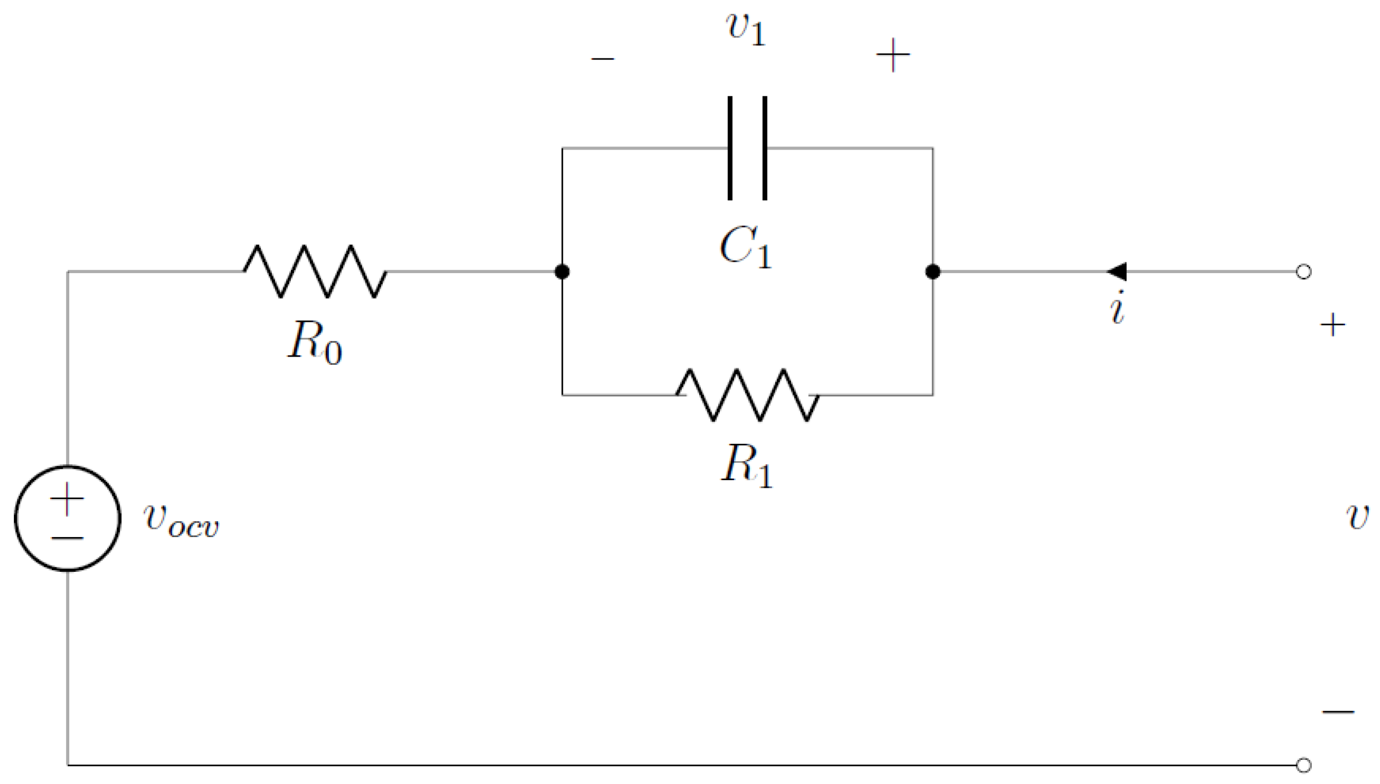
The following section summarizes the dynamic equations for a battery modeled by an extended equivalent circuit model (XECM) as depicted in Figure 3. Here, the equations of motion are introduced in Section 4.1.1. Afterwards, Section 4.1.2 introduces a battery heating model.

4.1.1. Local Voltage and Ion Concentration Dynamic Equations

The local voltage $v_1$ and ion concentration $\Delta z_1$ equations of motion are based on the parallel resistor–capacitor arrangement in Figure 3. The equations are given by first order lags with the current i as the control variable:

$$\begin{array}{cccc}\hfill {\dot{v}}_1& =-\frac{1}{R_1·C_1}\hfill & ·v_1\hfill & +\frac{1}{2·C_1}i,\hfill \end{array}$$

(22a)

$$\begin{array}{cccc}\hfill \Delta {\dot{z}}_1& =-\frac{1}{R_1·C_1}\hfill & ·\Delta z_1\hfill & +\frac{1}{2·C_1}i.\hfill \end{array}$$

(22b)

Here, $R_1$ and $C_1$ are the resistance and capacity, respectively. It should be noted that $R_1$ and $C_1$ are functions of the battery temperature (Section 4.1.2).

In addition, we have the total ion concentration z dynamic equation, also called state of charge (SoC), that is only dependent on the current:

$$\dot{z}=\frac{1}{Q}i.$$

(23)

Here, Q is the battery capacity.

4.1.2. Battery Heating

As an extension to the standard XECM in Section 4.1.1, we also model the heating of the battery when a current is applied. This heating can again be formulated by an equation of motion for the battery temperature $T_{batt}$ that is mainly influenced by the square of the applied current:

$${\dot{T}}_{batt}=k_1·i^2+k_2·\left(T_{amb}-T_{batt}\right).$$

(24)

The coefficients $k_1=\frac{k_{R_0}·R_0}{m_{batt}c}$ as well as $k_2$ are again parameters of the battery, while $T_{amb}$ is the ambient temperature. It should be noted that $k_{R_0}$ is the considered uncertainty and is a scaling factor for the lumped resistance term $R_0$. It is uniformly distributed as follows:

$$k_{R_0}\in \mathcal{U}\left(0.8;1.2\right),\mu =1,\sigma \approx 0.1155.$$

(25)

Thus, the lumped resistance term can vary up to $\pm 20\%$, which refers to the uncertainty that is introduced to the system when identifying the parameter. Take into account that we choose this parameter as the uncertain value as it is also the main contributor to the battery temperature increase, which we want a robust trajectory against. Additionally, it should be noted that the uncertainty definition in Equation (25) implies using a Uniform pdf as the proposal distribution in Algorithm 2.

For the CC optimization, we want to achieve that the following probability for the battery temperature is always fulfilled:

$$\mathbb{P}\left[0^{\circ }C\le T_{batt}\le {40}^{\circ }C\right]\ge 0.999999.$$

(26)

This CC is implemented using the SubSim approach presented in Section 3.3 and the sigmoid approximation of the CC with the homotopy strategy presented in Section 3.2. We use this kind of probability as we want to assure that the battery is not damaged by a temperature that is too high, but also charges as optimally as possible without being too conservative. In addition, it might not be possible in general applications, due to other system constraints, to calculate a fully robust trajectory, which makes the use of CCs viable.

4.2. Problem Setup

The problem consists of two phases that model one charge and one discharge of the battery. The following initial boundary conditions ($IBC$;

Table 2. Initial boundary condition (IBC) of the optimization problem.

Phase	${\mathit{IBC}}_{\mathit{lb}}$	${\mathit{IBC}}_{\mathit{ub}}$
1	$[0,0,0.15,20]$	$[0,0,0.15,20]$

) for the states $\mathbf{x}=\left[\begin{array}{cccc}{v}_1& \Delta z_1& z& T_{batt}\end{array}\right]$ that define these conditions in the beginning of the first phase are as follows (these are assigned as inequality constraints in Equation (6)):

Furthermore, the final boundary conditions ($FBC$;

Table 3. Final boundary conditions (FBC) of the optimization problem.

Phase	${\mathit{FBC}}_{\mathit{lb}}$	${\mathit{FBC}}_{\mathit{ub}}$
1	$[0,0,0.95,-10]$	$[0.15,0.5,1.00,40]$
2	$[0,0,0.00,-10]$	$[0.15,0.5,0.15,40]$

) for the same states in all phases are defined as follows (again assigned as inequality constraints in Equation (6)):

It should be noted here that trying to e.g., enforce an equality constraint for the final boundary condition with only the mean robust control, as in Equation (7), might yield an infeasible OCP. In this case, a CC should be considered to model the final boundary condition or an inequality constraint (as used in this study) can be applied.

The states with their respective lower and upper bounds $x_{lb},x_{ub}$, and scaling $x_S$ are as given in

Table 4. States upper and lower bounds as well as scalings.

State	Description	${\mathit{x}}_{\mathit{lb}}$	${\mathit{x}}_{\mathit{ub}}$	${\mathit{x}}_{\mathit{S}}$
$v_1$	Local voltage	0	$0.15$	${10}^0$
$\Delta z_1$	Local concentration	0	1	${10}^0$
z	Total concentration	$0.05$	$0.95$	${10}^0$
$T_{batt}$	Battery temperature	$-10$	40	${10}^{-1}$

.

The controls with their respective lower and upper bounds $u_{lb},u_{ub}$, and scaling $u_S$ are defined as in

Table 5. Control upper and lower bounds as well as scalings.

Control	Description	${\mathit{u}}_{\mathit{lb}}$	${\mathit{u}}_{\mathit{ub}}$	${\mathit{u}}_{\mathit{S}}$
$i^{charge}$	Charge current	0	$3·Q$	${10}^{-1}$
$i^{discharge}$	Discharge current	$-3·Q$	0	${10}^{-1}$

.

Finally, the parameters and the constants of the optimization model are defined in

Table 6. Parameters and constants of the optimization model.

Value	Description	Reference
$T_{amb}$	Ambient Temperature	$20{}^{\circ }\mathrm{C}$
$m_{batt}c$	battery mass times specific heat capacity	$260\frac{J}{{}^{\circ }\mathrm{C}}$
$k_2$	convection coefficient of battery with ambient	$0.00001\frac{1}{s}$
$R_1$	Local Resistance	$fcn\left(T_{batt}\right)$
$R_0$	Lumped Resistance	$fcn\left(T_{batt}\right)$
$C_1$	Local Capacity	$fcn\left(T_{batt}\right)$
Q	Battery Capacity	$26Ah$

.

Finally, we consider the following cost function to minimize the cycle time:

$$J={\widehat{t}}_f^{\left(0\right)}.$$

(27)

This is a parameter cost that actually requires a trade-off between fulfilling the CC and finishing the cycle as fast as possible, due to the fact that a fast charging/discharging with large current yields a fast temperature increase.

5. Optimization Cases

This section covers the test cases for the CC–OC framework. At first, a single phase with only charging is looked at in Section 5.1 to get an overview of the problem characteristics. Then, Section 5.2 looks at a charge–discharge cycle. Generally, each phase has $N=125$ time discretization steps yielding NLP problem sizes of around 2000 optimization variables and constraints.

For the final results, which are depicted in the following, the scaling factor of the sigmoid CC approximation is $a=\pm 50$. This could be achieved in a single homotopy step for the results in Section 5.1 and with two homotopy steps for the results in Section 5.2. The homotopy begins with $a=\pm 1$ and has an intermediate step, in the second example, at $a=\pm 25$. In general, we use $n_s=10,000$ random samples to approximate the probability of the CC using the methods introduced in Section 3. The gPC expansion order is chosen to be three as this has shown to be viable for these kind of problems. The CC is defined as given in Equation (26). Take into account that the initial MCA solution fulfills the CC in Equation (26) with a probability of $97.5\%$. After this initial solution, we directly assign the desired probability, given in Equation (26), to the CC–OC and thus require one homotopy step.

In the following, we show the results obtained for the different SubSim level (“SSLevel”) runs with $p_0=0.1$ and $n_s=2500$ during the homotopy procedure. Here, the zeroth level is the basic MCA solution. The gPC order is chosen to be three, which was determined to be sufficient by comparing the accuracy of the expansion with MCA optimization runs.

5.1. Battery Charging Optimization

This section introduces the optimization of a single battery charge by looking at the general time-optimal OCP (Equation (27)).

In Figure 4, which depicts the probability of not fulfilling the CC, it can be seen that our desired probability level is fulfilled after the first SubSim level. This probability is calculated in a post-processing step using 1 million samples and the analytic indicator function in Equation (12): here, we get a level close to $0\%$ failures and thus the CC is, based on our sampling, fulfilled with a very high certainty. Indeed, the SubSim evaluates the failure probability to be $\mathbb{P}\left(\mathcal{F}\right)=2.0088·{10}^{-5}\%$ with a c.o.v. of $\nu =1.0052$. Thus, we fulfill our desired failure probability of ${10}^{-4}\%$ even though we have a slightly high c.o.v..

This can also be seen looking at Figure 5 that shows the fitted marginal distribution of the failure probability at the final point in time (i.e., the end time). This is the point where the violation is most likely to occur. Here, the already mentioned method of fitting a Beta pdf for the c.o.v. estimation by applying the theory in study [25] is used. The pdf is depicted in solid blue and plotted in the range of $[0,{\mathbb{P}}_{des}\left(\mathcal{F}\right)]$, which covers the range of the pdf and its probability until the maximal allowed failure probability. The mean value is depicted in dashed black. It is evident that the pdf fulfills our rare-event CC with high probability and thus we can be confident in the certainty of our result. To be specific, according to the SubSim and the Beta pdf of [25], the CC is fulfilled with almost $97\%$ certainty for our application.

In Figure 6, the current for the robust optimal result is shown. We can see that the current is mainly at its maximum bound for the MCA optimization (SSLevel: 0), while it decreases linearly from a general lower level to fulfill the tighter bounds of the desired rare-event probability in the SSLevel 1 run. The optimal time is slightly increased for the SSLevel 1.

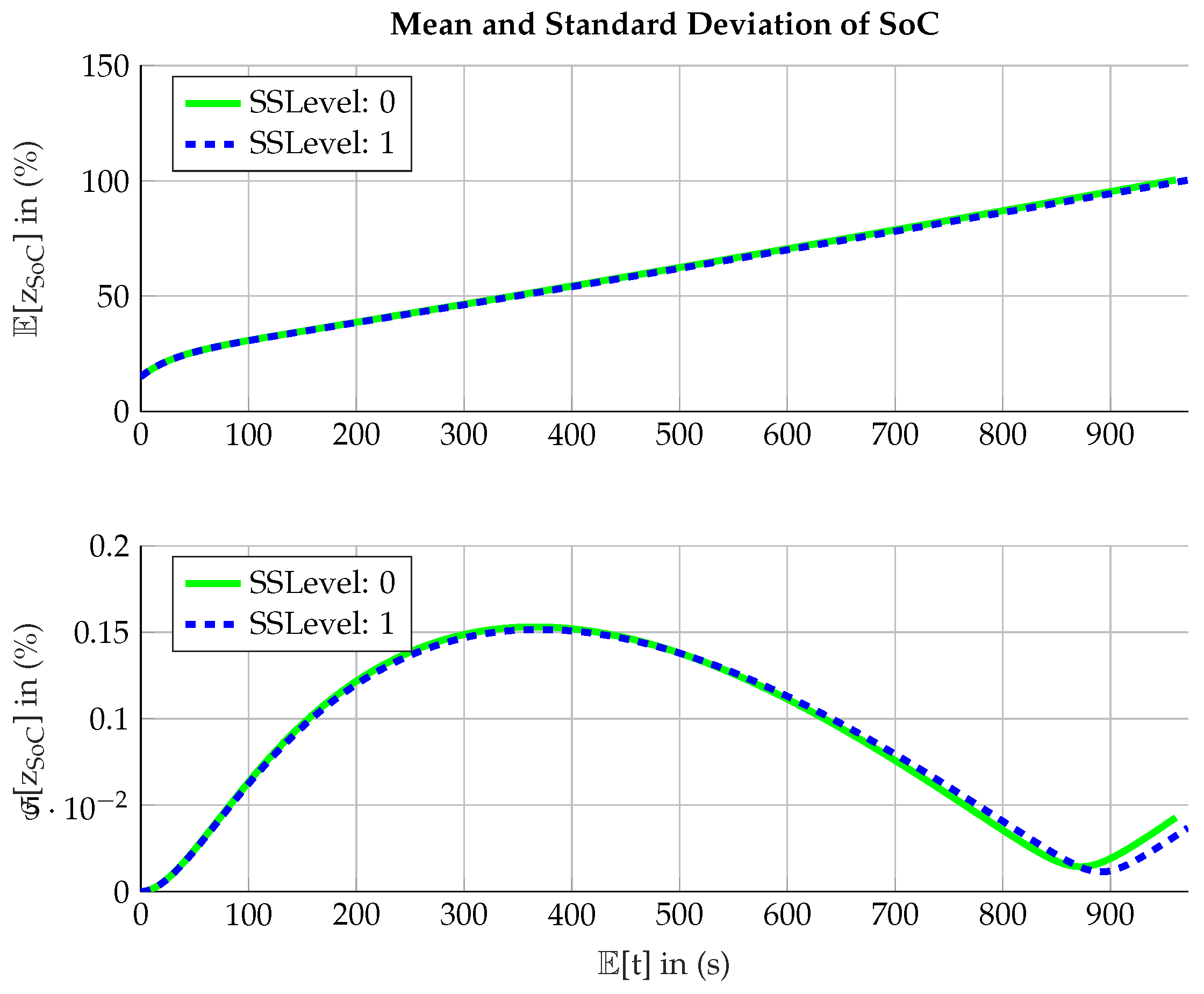
Finally, Figure 7 shows the development of the SoC for the mean value and the standard deviation. We observe a basically linear increase in the mean value reaching the desired charging level and a small standard deviation. Overall, the SoC is only subject to minor influences by the defined uncertainty that are mainly based on the temperature variations. Thus, although there is an uncertainty, we can still reach a similar charging level with the proposed robust open–loop optimal control (ROC) method. Furthermore, there are only minor differences between the different SubSim levels.

5.2. Battery Charge-Discharge Cycle Optimization

Within this section, we are looking at the full charge–discharge cycle: For this, Figure 8 shows the optimal current histories. In contrast to the single cycle, we can see that the current now is not reaching the maximal value anymore (78A; Section 4.2) and is also gradually decreasing over time. The differences between the SubSim levels are overall quite minimal but the same trend as for the results in Figure 6 can be observed, i.e., that the SubSim levels after the MCA have an overall lower level and are slightly longer.

Then, Figure 9 shows the fitted marginal distribution of the failure probability at the final point in time (i.e., the end time) once more. Once again, the pdf is plotted in the range of $[0,{\mathbb{P}}_{des}\left(\mathcal{F}\right)]$, i.e., we cover the part of the pdf and its probability until the allowed maximal failure probability. Although we can see that the failure probability is now twice as large in the mean as for only the charge cycle (Figure 5), we can still be certain regarding our confidence in fulfilling the CC (around $91.5\%$).

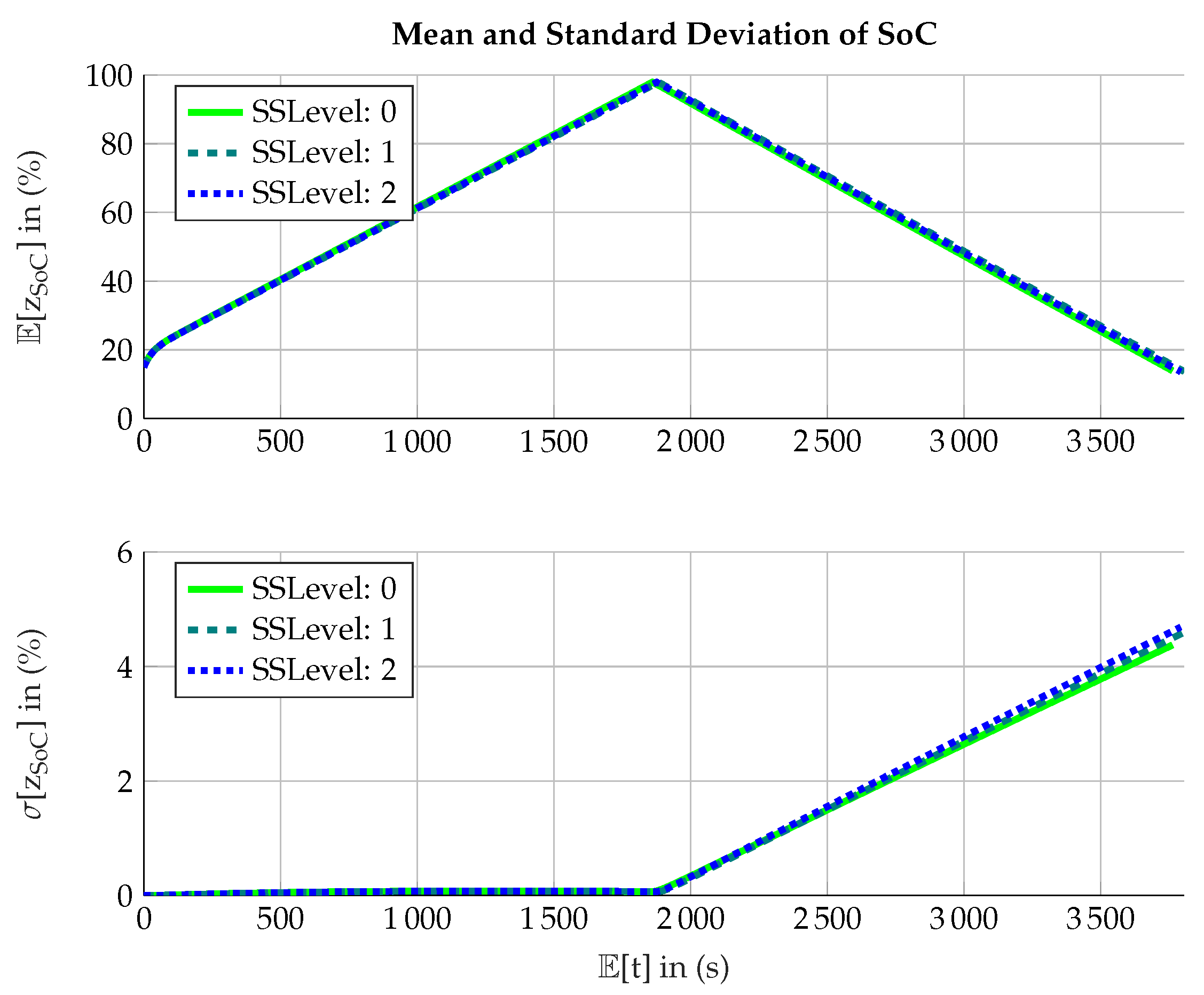
Now, Figure 10 shows the mean value of the SoC and its standard deviation. We can observe that the SoC is virtually independent of the SubSim level, but a major increase in the standard deviation can be seen, which is a consequence of the robust charging and the uncertainty. Generally, this increase is based on an increased standard deviation of the optimal time.

Finally, Figure 11 depicts the battery temperature mean value and mean value with an added standard deviation. It should be noted that, in this figure, the standard deviation is added with a factor of $k_{\sigma }=1.7321$: this value is chosen as it is exactly the value that yields the boundary value of the original uniform pdf if adding the standard deviation in Equation (25). As the optimization model is linear in the uncertainty, we can expect that the propagated uncertainty at the output is thus also almost linear. This is strengthened by Figure 11 as the solution that is offset by the factor $k_{\sigma }=1.7321$ is just violating the constraint at the end, which is based on the CC fulfillment that must not be $100\%$. Again, the level 1 SubSim yields a reduced exceedance with a longer charge time.

6. Conclusions

This paper presented an efficient method for ROC that relies on a CC–OC framework. In this framework, CCs are approximated by efficiently sampling from the gPC expansion. Therefore, a direct transcription method using the gPC expansion is applied for solving the OCP: by this, the gPC expansion can be evaluated in each optimization step as a matrix-vector operation and efficient sampling of the CC value, and thus its probability, is possible. In order to make the sharp CC bounds usable for Newton-type OC applications, the paper additionally introduced an approximation of CCs by means of sigmoids. This sigmoid approximation is gradually adapted using a homotopy strategy to reach a good approximation of the original sharp bound. Finally, the method of SubSim is applied to get the capability of calculating rare event failure probabilities. Overall, the applicability of the framework is shown using battery charge and discharge examples.

In the future, developments can be made combining the proposed method with distributed open–loop optimal control (DOC). The DOC framework can then be used to handle smaller sub-problems of the original OCP, which can be solved more efficiently. Here, also a distribution of the SubSim can be considered for improved efficiency.

Furthermore, more research should be directed into the suitable choice of the gPC expansion order to find a good response surface approximation for the evaluation of the CC. Here, especially the truncation errors of the gPC expansion as well as the SC evaluation must be considered. This is necessary to accurately calculate the probability of fulfilling the CC. In addition, e.g., a moment-matching optimization [27], which tries to find the best nodes-weights combination for the given problem, could be applied. Especially with a highly nonlinear model, larger orders of the gPC expansion must also be used, which decreases the efficiency. In the context of this large expansion order as well as a high-dimensional uncertainty space, further research must also be directed to efficient (adaptive) sparse grid implementations for the SC evaluation [19,28].

Additionally, in future applications, general pdfs can be introduced in the proposed method using the theory of arbitrary polynomial chaos [18,29] or Gaussian mixture models [30]. This could also be of special interest for the accurate choice of the SubSim evaluation points.

Finally, research can be directed into controlling the c.o.v. of the SubSim using the Beta pdf introduced in [25]. This can be beneficial to have a small dispersion of the data and thus high confidence in the calculated failure probability estimation and, consequently, the calculated robust optimal trajectories.

References

- Xiu, D.; Karniadakis, G.E. The Wiener-Askey Polynomial Chaos for Stochastic Differential Equations. SIAM J. Sci. Comput. 2002, 24, 619–644. [Google Scholar] [CrossRef]
- Vitus, M.P. Stochastic Control via Chance Constrained Optimization and its Application to Unmanned Aerial Vehicles. Ph.D. Thesis, Stanford University, Stanford, CA, USA, 2012. [Google Scholar]
- Zhao, Z.; Liu, F.; Kumar, M.; Rao, A.V. A novel approach to chance constrained optimal control problems. In Proceedings of the American Control Conference (ACC), Chicago, IL, USA, 1–3 July 2015; pp. 5611–5616. [Google Scholar] [CrossRef]
- Mesbah, A. Stochastic Model Predictive Control: An Overview and Perspectives for Future Research. IEEE Control Syst. 2016, 36, 30–44. [Google Scholar] [CrossRef]
- Diehl, M.; Bjornberg, J. Robust Dynamic Programming for Min–Max Model Predictive Control of Constrained Uncertain Systems. IEEE Trans. Autom. Control 2004, 49, 2253–2257. [Google Scholar] [CrossRef]
- Lu, Y.; Arkun, Y. Quasi-Min-Max MPC algorithms for LPV systems. Automatica 2000, 36, 527–540. [Google Scholar] [CrossRef]
- Villanueva, M.E.; Quirynen, R.; Diehl, M.; Chachuat, B.; Houska, B. Robust MPC via min–max differential inequalities. Automatica 2017, 77, 311–321. [Google Scholar] [CrossRef]
- Gavilan, F.; Vazquez, R.; Camacho, E.F. Chance-constrained model predictive control for spacecraft rendezvous with disturbance estimation. Control Eng. Pract. 2012, 20, 111–122. [Google Scholar] [CrossRef]
- Schaich, R.M.; Cannon, M. Maximising the guaranteed feasible set for stochastic MPC with chance constraints. IFAC-PapersOnLine 2017, 50, 8220–8225. [Google Scholar] [CrossRef]
- Zhang, X.; Georghiou, A.; Lygeros, J. Convex approximation of chance-constrained MPC through piecewise affine policies using randomized and robust optimization. In Proceedings of the 2015 54th IEEE Conference on Decision and Control (CDC), Osaka, Japan, 15–18 December 2015; pp. 3038–3043. [Google Scholar] [CrossRef]
- Au, S.K.; Beck, J.L. Estimation of small failure probabilities in high dimensions by subset simulation. Probab. Eng. Mech. 2001, 16, 263–277. [Google Scholar] [CrossRef]
- Au, S.K. Engineering Risk Assessment with Subset Simulation; Wiley: Hoboken, NJ, USA, 2014. [Google Scholar]
- Betts, J.T. Practical Methods for Optimal Control and Estimation Using Nonlinear Programming, 2nd ed.; Advances in Design and Control; Society for Industrial and Applied Mathematics (SIAM 3600 Market Street Floor 6 Philadelphia PA 19104): Philadelphia, PA, USA, 2010. [Google Scholar]
- Rieck, M.; Bittner, M.; Grüter, B.; Diepolder, J.; Piprek, P. FALCON.m User Guide, Institute of Flight System Dynamics, Technical University of Munich. 2019. Available online: www.falcon-m.com (accessed on 30 March 2019).
- Wächter, A.; Biegler, L.T. On the implementation of an interior-point filter line-search algorithm for large-scale nonlinear programming. Math. Program. 2006, 106, 25–57. [Google Scholar] [CrossRef]
- Wiener, N. The Homogeneous Chaos. Am. J. Math. 1938, 60, 897. [Google Scholar] [CrossRef]
- Xiu, D. Numerical Methods for sTochastic Computations: A Spectral Method Approach; Princeton University Press: Princeton, NJ, USA, 2010. [Google Scholar]
- Witteveen, J.A.; Bijl, H. Modeling Arbitrary Uncertainties Using Gram-Schmidt Polynomial Chaos. In Proceedings of the 44th AIAA Aerospace Sciences Meeting and Exhibit, Reno, Nevada, 9–12 January 2006. [Google Scholar]
- Xiu, D. Fast Numerical Methods for Stochastic Computations: A Review. Commun. Comput. Phys. 2009, 5, 242–272. [Google Scholar]
- Bittner, M. Utilization of Problem and Dynamic Characteristics for Solving Large Scale Optimal Control Problems. Ph.D. Thesis, Technische Universität München, Garching, Germany, 2016. [Google Scholar]
- Sherlock, C.; Fearnhead, P.; Roberts, G.O. The Random Walk Metropolis: Linking Theory and Practice Through a Case Study. Stat. Sci. 2010, 25, 172–190. [Google Scholar] [CrossRef]
- Bucklew, J.A. Introduction to Rare Event Simulation; Springer Series in Statistics; Springer: New York, NY, USA, 2004. [Google Scholar]
- Au, S.K.; Patelli, E. Rare event simulation in finite-infinite dimensional space. Reliab. Eng. Syst. Saf. 2016, 148, 67–77. [Google Scholar] [CrossRef]
- Papaioannou, I.; Betz, W.; Zwirglmaier, K.; Straub, D. MCMC algorithms for Subset Simulation. Probab. Eng. Mech. 2015, 41, 89–103. [Google Scholar] [CrossRef]
- Zuev, K.M.; Beck, J.L.; Au, S.K.; Katafygiotis, L.S. Bayesian post-processor and other enhancements of Subset Simulation for estimating failure probabilities in high dimensions. Comput. Struct. 2012, 92–93, 283–296. [Google Scholar] [CrossRef]
- Skötte, J. Optimal Charging Strategy for Electric Vehicles. Master’s Thesis, Chalmers University of Technology, Gothenburg, Sweden, May 2018. [Google Scholar]
- Paulson, J.A.; Mesbah, A. Shaping the Closed-Loop Behavior of Nonlinear Systems Under Probabilistic Uncertainty Using Arbitrary Polynomial Chaos. In Proceedings of the 2018 IEEE Conference on Decision and Control (CDC), Miami Beach, FL, USA, 17–19 December 2018; pp. 6307–6313. [Google Scholar] [CrossRef]
- Blatman, G.; Sudret, B. Adaptive sparse polynomial chaos expansion based on least angle regression. J. Comput. Phys. 2011, 230, 2345–2367. [Google Scholar] [CrossRef]
- Paulson, J.A.; Buehler, E.A.; Mesbah, A. Arbitrary Polynomial Chaos for Uncertainty Propagation of Correlated Random Variables in Dynamic Systems. IFAC-PapersOnLine 2017, 50, 3548–3553. [Google Scholar] [CrossRef]
- Piprek, P.; Holzapfel, F. Robust Trajectory Optimization combining Gaussian Mixture Models with Stochastic Collocation. In Proceedings of the IEEE Conference on Control Technology and Applications (CCTA), Mauna Lani, HI, USA, 27–30 August 2017; pp. 1751–1756. [Google Scholar]
Figure 1.
Product of two sigmoids with different scaling and offset parameters to approximate an uncertainty domain by box constraints.
Figure 2.
General behavior of subset simulation with modified Metropolis–Hastings algorithm and showing movement of the samples (red: in failure domain, green: not in failure domain) over the different subset levels with arc failure domains at edges.
Figure 3.
Schematics of Extended Equivalent Circuit Model (XECM) [26].
Figure 4.
Probability of fulfilling the chance constraint over time for charging.
Figure 5.
Estimation of failure probability density function from subset simulation for a final point on the optimization time horizon using a Beta distribution with mean value and probability density function area estimation until the allowed failure probability.
Figure 6.
Robust control history for the current as the command variable over time for charging.
Figure 7.
Mean and standard deviation value for state-of-charge over time for charging.
Figure 8.
Robust control history for the current as the command variable over time for charge–discharge cycle.
Figure 9.
Estimation of failure probability density function for charge–discharge cycle from subset simulation for the final point on an optimization time horizon using a Beta distribution with mean value and probability density function area estimation until the allowed failure probability.
Figure 10.
Mean and standard deviation value for state-of-charge over time for charge–discharge cycle.
Figure 11.
Mean battery temperature including the standard deviation interval provided by the underlying uniform parameter uncertainty over time for the charge–discharge cycle.