Implementation of Maximum Power Point Tracking Based on Variable Speed Forecasting for Wind Energy Systems

Abstract

In order to precisely control the wind power generation systems under nonlinear variable wind velocity, this paper proposes a novel maximum power tracking (MPPT) strategy for wind turbine systems based on a hybrid wind velocity forecasting algorithm. The proposed algorithm adapts the bat algorithm and improved extreme learning machine (BA-ELM) for forecasting wind speed to alleviate the slow response of anemometers and sensors, considering that the change of wind speed requires a very short response time. In the controlling strategy, to optimize the output power, a state feedback control technique is proposed to achieve the rotor flux and rotor speed tracking purpose based on MPPT algorithm. This method could decouple the current and voltage of induction generator to track the reference of stator current and flux linkage. By adjusting the wind turbine mechanical speed, the wind energy system could operate at the optimal rotational speed and achieve the maximal power. Simulation results verified the effectiveness of the proposed technique.

1. Introduction

Wind, used as widely distributed huge reserves of green energy [1], has dramatic increased in grid-connected power these years. Thus, to improve the efficiency of wind power system becomes an essential part, both to reduce the costs of wind power generation systems, and to increase the proportion of renewable energy in the national power grid. High efficiency, good robustness and low costs have become the research focus of wind energy harnessing.

Currently, the literature extensively investigates modeling effective wind turbine systems to optimize and effectively utilize the turbine power output through the maximum power point tracking (MPPT) technique. By the adoption of variable speed wind turbine (VSWT), adjusting the rotation speed of wind turbine rapidly according to the variable wind speed can achieve for high efficiency to harness wind source [2]. These technique adopted by MPPT controller mainly can be categorized into four types: by controlling of Tip Speed Ratio (TSR), adopting Power Signal Feedback (PSF) control, Perturb and Observe (P&O) method, and Optimal Torque Control (OTC) method. TSR is a constant value which is dependent of wind velocity. It is the only parameter that can be set to provide the maximum power output from wind which is related to rotor radius and the blades rotational speed [3]. Such method needs two sensors to measure the wind and turbine speeds by an anemometer and a tachometer respectively for that both wind speed and rotational speed are feedback signals [4]. Compared to TSR (nomenclature can be seen in

Table 1. Acronyms and nomenclature.

BA	bat algorithm
MPPT	maximum power point tracking
VSWT	variable speed wind turbine
PSF	adopting power signal feedback
TSR	tip speed ratio
OTC	optimal torque control
FIS	fuzzy inference system
ELM	extreme learning machine
SLFNN	single-hidden layer feed-forward neural networks
MAE	mean absolute error
MSE	mean square error
VOC	voltage oriented control
P&O	perturb and observe

), PSF only uses one sensor to measure rotational speed. Error between measured turbine power and reference power is delivered to the controller, then the output power is adjusted to the reference value. The efficiency is good and the reliability is better than TSR [5]. While the P&O method does not necessarily need any sensor beside the electrical measurement devices, its reliability is strong but efficiency is not good. The Optimal Torque Control (OTC) extracts optimum torque by measuring angular velocity [6], which is similar to PSF control yet adopts mechanical torque equation.

However, these conventional techniques fail to consider that the wind speed is a discrete nonlinear parameter set which is not compliant to a certain law of variation. That requires the anemometers to measure wind velocity in time and the controller should also respond quickly to the wind speed fluctuation, then drives the mechanical rotor to rotate with the optimized direction and speed. Usually the measurements and controlling process should not exceed one second to harness the wind energy in highest efficiency [7]. Yet in large-scale wind turbines, anemometers and controllers have large volume and great inertia, leading to a slow response [8]. Therefore, typically when a rotor speed instruction has not completed, the controller should execute in an opposite direction. In this way, the wind turbine is more likely to have mechanical fatigue. Besides, because of the hysteresis effect, the current optimal tracking point is not the current maximum power point.

Such problems are noticed by scholars in recent years, with the development of computational intelligence and numerical optimization, some novel MPPT frameworks are also proposed to tackle this issue. These framework often involves: the fuzzy inference system (FIS), taking multi-objectives into account [9]; nonlinear control [10], with Boukhezzar et al. adapts a two-mass model with a wind speed estimator for variable-speed wind turbine control [11]; robust control, via controlling the rotor angular speed to control the tip-speed ratio [12]; adaptive control [13] and the like. Some scholars even proposed hybrid models with the combination of artificial intelligence algorithm and conventional control methods to achieve a higher efficiency [14]. Though it can effectively deal with high non-linearity of wind turbines, the training process is indeed time-costing and introduces a huge amount of iteration parameters like weights and bias into systems [15]. In order to avoid generating these parameters and to save hardware, here we consider extreme learning machine (ELM) to forecasting wind velocity, which do not need to use back-propagation method to updates weights and thresholds and only the linear least square solution is needed [15]. With the prediction scheme, a novel controlling strategy to intervene the hysteresis effect in both wind speed measurement and controlling process is proposed in this paper.

The proposed controlling strategy can be concluded into three steps, first is to optimize the weights and thresholds of extreme learning machine (ELM) by bat algorithm (BA) to forecast the short–term wind speed, since the random distributed weights and bias of traditional ELM algorithm are likely to be not convergent [16]. The second is that we adapt the forecasting values to calculate the optimal reference rotational speed based on MPPT algorithm. Meanwhile the anemometer would measure the current wind velocity thus to feed the input of BA-ELM. Finally the state feedback control and optimal control technique will be implemented in wind energy conversion system, to achieve maximal power point thus the current asynchronous machine torque can achieve high efficiency [17].

The outline of rest is organized as follows. Section 2 describes the wind energy conversion system. Section 3 introduces the detailed design procedure of speed forecasting method with BA-ELM for wind energy conversion system. Section 4 presents the state feedback controller for induction machine with the MPPT algorithm. The simulation results are presented in Section 5. Finally, some comments conclude this work in Section 6.

2. Wind Energy Conversion System

The wind energy conversion system is a high nonlinear and complex coupled system. The system comprises of the wind turbine, transmission device, induction machine and converters [18]. The basic components and general scheme of a wind energy system are shown in Figure 1, which contain the following main parts:

• Wind turbine, which is a installation capturing wind energy by blades and transferring the wind kinetic power to mechanical torque;
• Induction machine, which can convert the power from the mechanical side into the electrical side.
• Gearbox and shaft, which is a transmission device to adapt the rotation speed for the generator;
• Power converters, it is composed of the grid side inverter and the machine side rectifier, connected by a DC-bus.

The following subsections will focus on the wind turbine model and induction machine model.

2.1. Wind Turbine Model

The wind turbine extracts power by the wind blades in the turbine nacelle, then converts it into mechanical power. The wind kinetic power can be formulated as follows:

$$P_w=\frac{1}{2}\rho \pi R^2{V}_w^3$$

(1)

where $P_w$ represents the power input of wind turbine, R determines the radius of blades, $V_w$ indicates the wind speed.

The tip speed ratio $\lambda$ can be expressed by

$$\lambda =\frac{R{\omega }_r}{V_w}$$

(2)

where ${\omega }_r$ represents the rotor speed.

The power extracted from the wind is

$$P_m=\frac{1}{2}{C}_p(\lambda ,\beta )\rho \pi R^2{V}_w^3$$

(3)

where $P_m$ represents the mechanical power, $C_p(\lambda ,\beta )$ is a non-linear power coefficient depending on the design of turbine [19], which is:

$$C_p(\lambda ,\beta )=0.5176(\frac{116}{{\lambda }_i}-0.4\beta -5)e^{-\frac{21}{{\lambda }_i}}+0.0068\lambda$$

(4)

with

$$\frac{1}{{\lambda }_i}=\frac{1}{\lambda +0.08\beta }-\frac{0.035}{{\beta }^3+1}$$

(5)

where $\beta$ is the blade pitch angle. The power coefficient is a nonlinear function of tip speed ratio $\lambda$ and the blade pitch angle $\beta$, and its curve is plotted in Figure 2.

It can be seen that two points can be concluded to extract more power in the wind energy system [20], which are:

(a)

When the blade pitch angle $\beta$ does not change, the peak values of power coefficiency $C_p(\lambda ,\beta )$ corresponds to a unique tip speed ratio $\lambda$, where the conversion of wind energy is expected.

(b)

As the blade pitch angle $\beta$ increases, the wind energy use coefficient $C_p(\lambda ,\beta )$ decreases obviously. Thus for tracking more wind power, $\beta$ should be set into a small value.

The torque $T_L$ caused by the wind turbine can be computed as

$$T_L=\frac{P_{\mathrm{m}}}{{\omega }_r}=\frac{1}{2}\rho \frac{C_p(\lambda ,\beta )}{\lambda }\pi R^3{V}_w^2$$

(6)

From Equation (6), it can be noticed that the turbine $T_L$ is related to the wind speed $V_w$ and the characteristics of the turbine, that is the power coefficiency $C_p(\lambda ,\beta )$.

2.2. Induction Machine Model

2.2.1. Mechanical Equations

In the block wind turbine blades, the aerodynamic torque model can be used to describe dynamic relationship between the high-speed rotor shaft and the low-speed axial-flow fan of the wind turbine, which is composed of a spring and a damper. Formulations for the system can be established as follows:

$$J_m{\dot{\omega }}_r=T_{\mathrm{e}}-f_r{\omega }_r-T_L$$

(7)

where $J_m$ represents the rotary inertia of wind turbine pales.

2.2.2. State Space Equation of the Induction Machine Motor

The state space equation of induction machine in the well-known inductor part flux reference frame ($\alpha$,$\beta$) can be expressed as follows [21]:

$${\dot{i}}_{s\alpha }=-c_1{i}_{s\alpha }+c_2{c}_3{\psi }_{r\alpha }+c_{3}p{\omega }_r{\psi }_{r\beta }+\frac{u_{s\alpha }}{c_4}$$

(8)

$${\dot{i}}_{s\beta }=-c_1{i}_{s\beta }+c_2{c}_3{\psi }_{r\beta }-c_{3}p{\omega }_r{\psi }_{r\alpha }+\frac{u_{s\beta }}{c_4}$$

(9)

$${\dot{\psi }}_{r\alpha }=c_5{i}_{s\alpha }-c_6{\psi }_{r\alpha }-p{\omega }_r{\psi }_{r\beta }$$

(10)

$${\dot{\psi }}_{r\beta }=c_5{i}_{s\beta }-c_6{\psi }_{r\beta }+p{\omega }_r{\psi }_{r\alpha }$$

(11)

$$T_{\mathrm{e}}=\frac{p{M}_{sr}}{L_r}(i_{s\beta }{\psi }_{r\alpha }-i_{s\alpha }{\psi }_{r\beta })$$

(12)

where $u_{s\alpha }$ and $u_{s\beta }$ are the stator voltages, $i_{s\alpha }$ and $i_{s\beta }$ are the stator currents, ${\psi }_{r\alpha }$ and ${\psi }_{r\beta }$ are the rotor fluxes, p is the number of pole pairs, $M_{sr}$ is the mutual inductance, $L_r$ is the rotor inductance, $T_e$ is the electromagnetic torque. Moreover, the variables $c_1,c_2,c_3,c_4,c_5,c_6$ are defined as follows

$$c_1=\frac{R_s+R_r\frac{M_{sr}^2}{L_r^2}}{\sigma L_s},c_2=\frac{K}{T_r},c_3=K,c_4=\sigma L_s,c_5=\frac{M_{sr}}{T_r},c_6=\frac{1}{T_r}$$

with the related parameters $T_r,\sigma ,K$ are

$$T_r=\frac{L_r}{R_r},\sigma =1-\frac{M_{sr}^2}{L_s{L}_r},K=\frac{M_{sr}}{\sigma L_r}$$

where $R_s$ is stator resistance, $R_r$ is rotor resistance, $L_s$ is stator inductance.

Substitute Equation (12) into Equation (7), the dynamic equation can be expressed by the following form

$$\dot{{\omega }_r}=c_7({\psi }_{r\alpha }{i}_{s\beta }-{\psi }_{r\beta }{i}_{s\alpha })-\frac{f_r}{J_m}{\omega }_r-\frac{T_L}{J_m}$$

(13)

with $c_7=\frac{p{M}_{sr}}{J_m{L}_r}$ is a known constant.

2.2.3. Current Flux Model

In the induction machine model, the stator voltage and stator current can be measured, while the secondary flux can not be measured. Here, the current flux model is proposed to estimate the value of secondary flux. From voltage equation and flux equation of induction machine, the flux current model of induction machine is given as follows

$$\frac{d{\psi }_r}{dt}=-\frac{1}{T_r}{\psi }_r+\frac{M_{sr}}{T_r}{i}_s-j\left({\omega }_{mr}-p{\omega }_r\right){\psi }_r$$

(14)

where ${\psi }_r$ is the induced-part flux, $i_s$ is inductor current, ${\omega }_{mr}$ is the induced-part flux vector rotational speed, j is the imaginary unit. This equation represents the so-called “current model” of the induction machine.

3. Wind Speed Forecasting

As an anticipatory control strategy, predict wind velocity is more conducive to smooth the output power of wind turbines, since the power generation process is a complex nonlinear process, which will be affected by the wind speed and torque of the power generator. Besides, wind speed forecasting can estimate daily output of wind turbines in advance, and improve the planning ability of wind farms for electric power transmission and distribution. In addition, the maximum power point tracking can be achieved precisely by wind forecasting even without anemometers. Considering that there is a significant time-lag in the wind speed measurement of wind turbines for the anemometers’ inertia is great, suitable prediction model should be chosen from the model base according to certain principles. Here we build a hybrid prediction model of wind speed on the basis of applying the modified bat algorithm (BA) to optimize the initial weights in the layers of extreme learning machine (ELM). The prediction model can predict the future state of wind velocity on the basis of the estimated mechanical torque from the output of WES model, so as to settle down the problem of system lag from measurement of the anemometer. Thus to keep correspondence with current wind speed by adapting the mechanical speed ${\omega }_r$ mentioned above from blade shafts to predict the one-step wind speed, current maximum power can be tracking in higher accuracy which eliminates the effect of the system lag.

3.1. BA Algorithm

The bat algorithm (BA) is a novel metaheuristic algorithm adapted in prediction model is to optimize the input weights between layers of the studied training network [22]. Given a data set of of historical wind speed input to the network, the short term wind speed forecasting will perform as the output of prediction system.

The BA rules can be concluded as the real-time dynamic adjustment of the location, loudness and pulse emission of the virtual BA bats when hunting and foraging, bats change the frequency, loudness and pulse emissivity, and choose the best solution until the end specified iteration loop or achieve specified accuracy. Here we denote $y^t$ to be the bat positions, with the parameter t is the current iteration number. $f_i$ as the pulse frequency in a range [$f_{min}$, $f_{max}$], and $v_i$ is the velocities of bats. Initially each bat is assigned with a random frequency. An iterative loop is presented as follows:

$$f_i=f_{min}+(f_{max}-f_{min})\beta ,i=0,1,\cdots ,N-1$$

(15)

$${\mathrm{v}}_i^t={\mathrm{v}}_i^{t-1}+({\mathrm{y}}_i^t-y_{*})f_i,i=0,1,\cdots ,N-1$$

(16)

$${\mathrm{y}}_i^t={\mathrm{y}}_i^{t-1}+{\mathrm{v}}_{\mathrm{i}}^{\mathrm{t}},i=0,1,\cdots ,N-1$$

(17)

In the above formulation, $\beta \in [0,1]$, parameter N denotes specified loop accounts which end the iteration loop. Here the newest obtained position ${\mathrm{y}}_N^t$ will be evaluated with the fitness function to determine whether the solution exhibits the best current performance.

3.2. BA-ELM Network

Extreme Learning Machine (ELM) is a supervised learning algorithm originated from single-hidden layer feed-forward neural networks (SLFNN) proposed by Guangbin Huang [15], and it achieves high precision in the performance of classification and forecasting. Unlike other gradient-based learning algorithms, the main idea is that the weights between the input layer and the hidden layer, the bias of the hidden layer of ELM do not need to be adjusted. The solution is very efficient in that only the least norm and the least square solution are needed (ultimately resolved into Moore-Penrose inverse problem). Therefore, the algorithm has the advantages of using very few training parameters and achieving extremely fast speed [23].

Here for standard SLFNN, the constructed model is formulated as following [24].

$$\sum _{i=1}^{\tilde{N}}g\left({\mathrm{w}}_{\mathrm{i}}·{\mathrm{x}}_j+b_i\right){\beta }_i=t_j.j=1,2,\dots ,N$$

(18)

$\widehat{t_j}(w,\beta ,b)={[\widehat{t_{1j}}\cdots \widehat{t_{mj}}]}_{m\times 1}^T$

$$\begin{array}{c}\hfill ={[\sum _{i=1}^l{\beta }_{i1}g(w_1{X}_j+b_i)\cdots \sum _{i=1}^l{\beta }_{im}g(w_1{X}_j+b_i)]}_{m\times 1}^T,\end{array}$$

(19)

Which:

$$X_j={\left[\begin{array}{cccccc}{X}_{1j}& X_{2j}& X_{3j}& ···& X_{n-1j}& X_{nj}\end{array}\right]}^T$$

(20)

In the above formulation, $w_i$ denotes the weights between the input and the hidden layer. $X_j$ denotes the inputs historical wind speed data. $b_i$ denotes the bias. In addition, $g\left(x\right)$ denotes the activate function. ${\beta }_i$ which equals to ${\left({\beta }_{ij}\right)}_{\widehat{N}\times M}$, represents the weight matrix between the hidden layer and the output layer [4]. Here the above formulation can also be denoted as:

$$H\beta =T$$

(21)

H is the hidden layer output matrix of neural network. The equation has a unique solution when H is reversible (that means the number of hidden layers equals to the number of input data). While in most cases, the number of hidden layers is far less than the number of inputs. Common solutions to solve this problem include the gradient descend method to iterate parameters. However, it easily falls into the problem of over-trained and time-costing. To overcome its weakness, the literature points out that a lot of experiments show that H do not need to be adjusted, considering that adjusting input weights and biases of hidden layer will bring no possible gains [25]. Thus in ELM, when the input weights and biases are set once for all, the formulation (21) equals to find the linear least square solution for formulation (22).

$$∥H\widehat{\beta }-T∥=\underset{\beta }{min}∥H\beta -T∥$$

(22)

The detailed ELM training process can be found in [15]. Since the hidden layer nodes are pre-allocated and input weights and biases remain unchanged, some initial weights and biases are likely to remain non-optimized values [26]. For example, randomly allocated input weights might be zero, thus some hidden layer nodes would fail, leading that the model cannot converge or a slow convergence. To optimize these parameters, BA is introduced to optimize the weights and thresholds of ELM.

The BA-ELM training process can be concluded into two steps. First is to optimize the initial weights (w,$\beta$), and biases of the hidden layer b with the usage of bat algorithm. Second is to train the constructed ELM with these parameters and find the linear least square solution. The structure of BA-ELM is shown in Figure 3.

When running an iteration loop of BA, the fitness function will be invoked to update for the current best weights and thresholds, which aims to reduce the error between the predicted value and the actual wind speed value. Thus the current best of these parameters will be updated and substituted into ELM when an iteration of BA finished. Then the iteration loop of BA will stop when satisfy the objective tolerance of BA.

To evaluate the errors between the actual wind velocity and predicted ones, here two percentage error indexes are employed: mean absolute error (MAE), and the mean square error (MSE). In addition, the proposed BA-ELM are compared with traditional ELM, the promoting percentages are defined as follows:

$${\xi }_{MAE}=\left|\frac{MA{E}_1-MA{E}_2}{MA{E}_1}\right|\times 100\%$$

(23)

$${\xi }_{MSE}=\left|\frac{MS{E}_1-MS{E}_2}{MS{E}_1}\right|\times 100\%$$

(24)

Therefore we can output the forecasting wind speed at the end of our training process. The maximum rotor speed $w_{r,opt}$, can be deduced by applying Equation (5), which is a control signal to obtain the optimal tip speed ratio.

For the effective reduction of prediction error, the short-term wind speed prediction technique is applied in our model. Due to the uncertainty of system disturbance, it is necessary to improve the accuracy of the model and performance index in real time. The implementation of the ideology could be realized by solving the linear least square problem of $\beta$ and T. In each step, the real time output values of the system are detected and compared with the predicted values to correct the prediction error. When the system is influenced by such factors as the non-linearity, interference, adaptation of constructed model and the like, feedback compensation will correct the prediction output in time to make the optimization.

To verify the prediction accuracy of proposed BA-ELM network, we choose two indicators to test the precision of multi-step forecasting: the mean absolute error (MAE) and the mean square error (MSE). Training and testing data collected from three sites of different wind farms.

The speed forecasting results with BA-ELM algorithm is shown in

Table 2. Forecasting Performance of Modified ELM.

		ELM		BA-ELM		Percentage Improvement
		1-Step	2-Step	1-Step	2-Step		1-Step	2-Step
Site 1	MAE	0.138	0.233	0.109	0.193	${\xi }_{MAE}$	21.014	17.167
	MSE	0.055	0.062	0.037	0.060	${\xi }_{MSE}$	32.727	3.226
Site 2	MAE	0.159	0.245	0.127	0.236	${\xi }_{MAE}$	20.126	3.673
	MSE	0.047	0.079	0.039	0.069	${\xi }_{MSE}$	17.021	12.658
Site 3	MAE	0.175	0.244	0.132	0.40	${\xi }_{MAE}$	24.751	1.639
	MSE	0.026	0.108	0.025	0.086	${\xi }_{MSE}$	3.846	20.370

. Here two points can be concluded:

(1)

Single step wind speed forecasting of ELM and BA-ELM is more accurately compared to two-step forecasting, which indicates BA-ELM achieves high precision in shorter term forecasting.

(2)

Both networks can get good training and testing accuracy in forecasting. With bat algorithm to optimize the input weights and thresholds, BA-ELM is more inclined to obtain higher precision according to the MAE and MSE indexes, which illustrates that BA could improve the forecasting performance of ELM.

4. Controller Design

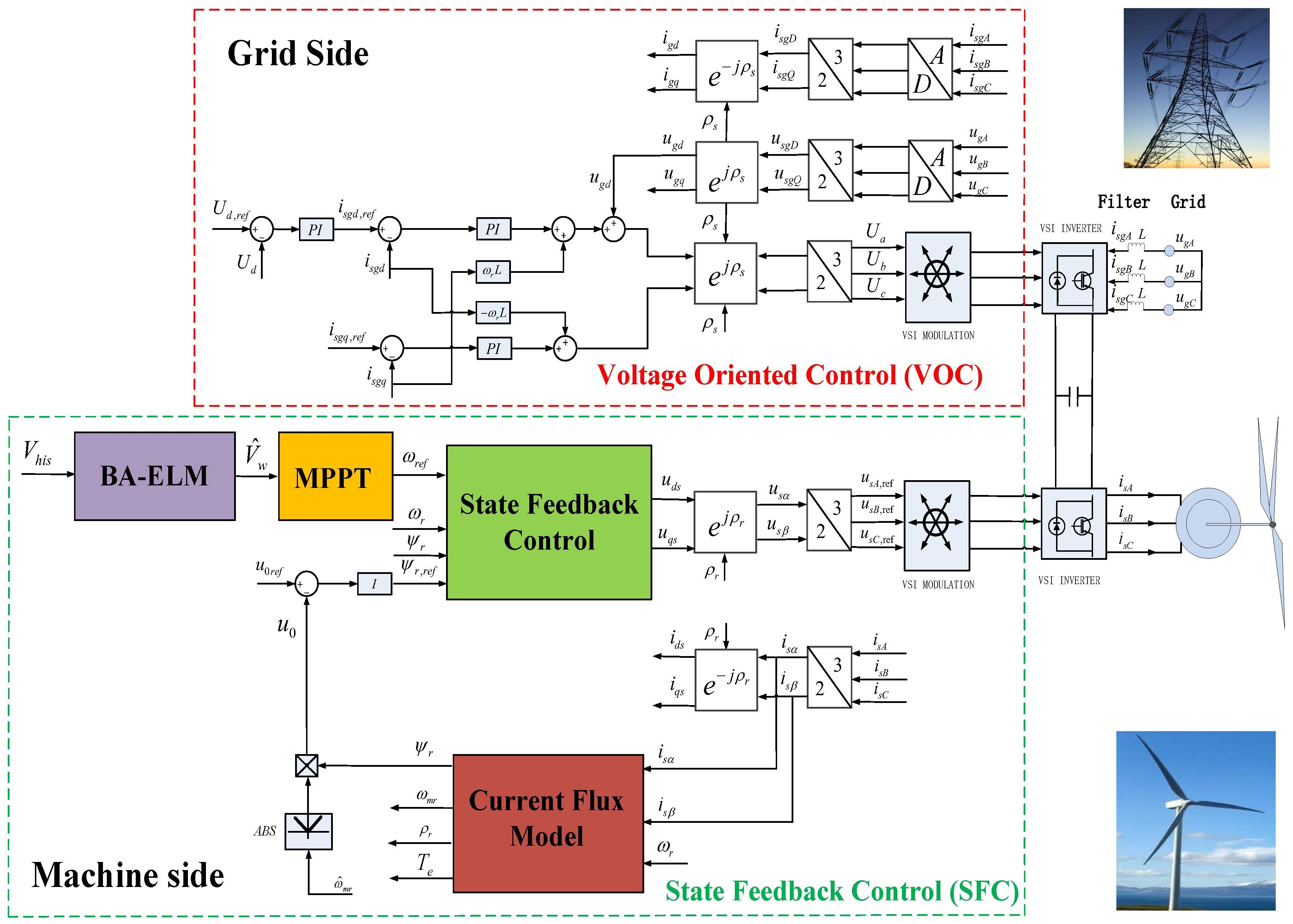
In order to achieve the MPPT control, the state feedback controller is designed by measuring the stator current and flux linkage compared with the desired current and flux reference. Considering the time lag in the turbine’s wind speed measurement, we adopt the turbine mechanical speed ${\omega }_r$ from blade shafts to predict the one-step wind speed $V_w$ [27]. The rotor flux is estimated with current flux model. For gird side, the voltage oriented control (VOC) is proposed. The overall control scheme for wind turbine system is shown in Figure 4. This figure contain two main parts: Grid Side and Machine Side. The Grid Side was designed with Voltage Oriented Control strategy. The Machine Side was designed by combined BA-ELM algorithm, MPPT and State Feedback Control strategy together.

4.1. MPPT Control Objective

From Equation (4), we can deduce that the MPPT algorithm should be applied to extract the maximum power from the wind turbine when the rotor speed is below the rated speed [28]. Moreover, a rotor power control mechanism should be activated when the rotor speed exceeds the speed of rated power. On account that different wind speed corresponds to unique optimal turbine speed, and the maximum power point is expected so that the power can be extracted as much as possible.

From Equation (2), the reference of generator speed is calculated by the optimal tip-speed ratio ${\lambda }_{opt}$, which is

$${\omega }_{r,opt}=\frac{{\lambda }_{opt}{V}_w}{R}$$

(25)

Currently, the wind speed used in the control system is usually measured with an anemometer. While in practical, the wind speed is changeable parameters [29]. In this paper, to record its real time value and to optimize the power output, the estimated effective wind speed ${\widehat{V}}_w$ is obtained with wind speed forecasting method mentioned above.

The block diagram of the MPPT technique is presented in Figure 5. It can be seen that the low pass filter was added to give a clear reference value of generator speed, which can avoid the turbulence of turbine mechanics.

4.2. Control System Design for Machine Side

4.2.1. Internal Loop Design

To represent the internal loop, rewrite the model from the model ($\alpha ,\beta$) stationary reference frame (8)–(12) to ($d,q$) rotary reference frame is given as follows:

$${\dot{i}}_{ds}=-c_1{i}_{ds}+{\omega }_{mr}{i}_{qs}+c_2{c}_3{\psi }_{dr}+c_{3}p{\omega }_r{\psi }_{qr}+\frac{u_{ds}}{c_4}$$

(26)

$${\dot{i}}_{qs}=-c_1{i}_{qs}-{\omega }_{mr}{i}_{ds}+c_2{c}_3{\psi }_{qr}-c_{3}p{\omega }_r{\psi }_{dr}+\frac{u_{qs}}{c_4}$$

(27)

$${\dot{\psi }}_{dr}=c_5{i}_{ds}-c_6{\psi }_{dr}+\left({\omega }_{mr}-p{\omega }_r\right){\psi }_{qr}$$

(28)

$${\dot{\psi }}_{qr}=c_5{i}_{qs}-c_6{\psi }_{qr}-\left({\omega }_{mr}-p{\omega }_r\right){\psi }_{dr}$$

(29)

$$\dot{{\omega }_r}=c_7\left({\psi }_{dr}{i}_{qs}-{\psi }_{qr}{i}_{ds}\right)-\frac{f_r}{J_m}{\omega }_r-\frac{T_L}{J_m}$$

(30)

where ${\omega }_{mr}$ is the rotating speed of the reference frame, which can be chosen arbitrarily, if we choose:

$$\frac{d{\rho }_r}{dt}={\omega }_{mr}=p{\omega }_r+c_5\frac{i_{qs}}{{\psi }_{dr}}=p{\omega }_r+\frac{M_{sr}}{T_r}\frac{i_{qs}}{{\psi }_{dr}}$$

(31)

Then Equation (29) will become

$${\dot{\psi }}_{qr}=-\frac{1}{T_r}{\psi }_{qr}$$

(32)

It is obvious that ${\dot{\psi }}_{qr}$ converge to zero exponentially, which means that ${\psi }_r={\psi }_{dr}$, then the state equations of LIM will become:

$${\dot{i}}_{ds}=-c_1{i}_{ds}+p{\omega }_r{i}_{qs}+c_5\frac{i_{qs}^2}{{\psi }_r}+c_2{c}_3{\psi }_r+\frac{u_{ds}}{c_4}$$

(33)

$${\dot{i}}_{qs}=-c_1{i}_{qs}-p{\omega }_r{i}_{ds}-c_5\frac{i_{ds}{i}_{qs}}{{\psi }_r}-c_{3}p{\omega }_r{\psi }_r+\frac{u_{qs}}{c_4}$$

(34)

$${\dot{\psi }}_r=c_5{i}_{ds}-c_6{\psi }_r$$

(35)

$${\dot{\rho }}_r=p{\omega }_r+c_5\frac{i_{qs}}{{\psi }_r}$$

(36)

$$\dot{{\omega }_r}=c_7{\psi }_r{i}_{qs}-\frac{f_r}{J_m}{\omega }_r-\frac{T_L}{J_m}$$

(37)

Now, the two control inputs $u_{ds}$ and $u_{qs}$ are designed through a state feedback as follows:

$$u_{ds}=c_4\left[-p{\omega }_r{i}_{qs}-c_5\frac{i_{qs}^2}{{\psi }_r}-c_2{c}_3{\psi }_r+v_{ds}\right]$$

(38)

$$u_{qs}=c_4\left[p{\omega }_r{i}_{ds}+c_5\frac{i_{ds}{i}_{qs}}{{\psi }_r}+c_{3}p{\omega }_r{\psi }_r+v_{qs}\right]$$

(39)

where $v_{ds}$ and $v_{qs}$ are additional control inputs that will be designed in the following stages.

Subtract Equations (38) and (39) in the induction machine model (33)–(37), we obtain the following equations:

$${\dot{i}}_{ds}=-c_1{i}_{ds}+v_{ds}$$

(40)

$${\dot{i}}_{qs}=-c_1{i}_{qs}+v_{qs}$$

(41)

$${\dot{\psi }}_r=c_5{i}_{ds}-c_6{\psi }_r$$

(42)

$${\dot{\rho }}_r=p{\omega }_r+c_5\frac{i_{qs}}{{\psi }_r}$$

(43)

$$\dot{{\omega }_r}=c_7{\psi }_r{i}_{qs}-\frac{f_r}{J_m}{\omega }_r-\frac{T_L}{J_m}$$

(44)

Using PI algorithm to design the control inputs $v_{ds}$ and $v_{qs}$, we obtain:

$$v_{ds}=-k_{pd}\left(i_{ds}-i_{ds,ref}\right)-k_{id}\underset{0}{\overset{t}{\int }}\left(i_{ds}-i_{ds,ref}\right)d\tau$$

(45)

$$v_{qs}=-k_{pq}\left(i_{qs}-i_{qs,ref}\right)-k_{iq}\underset{0}{\overset{t}{\int }}\left(i_{qs}-i_{qs,ref}\right)d\tau$$

(46)

In this subsection, the state feedback terms are used to decoupling the system. Then, two PI controllers are proposed to achieve current tracking. The two desired currents $i_{ds,ref}$ and $i_{qs,ref}$ will be designed in the next subsection.

4.2.2. External Loop Design

In this section, we design the desired current $i_{ds,ref}$ and $i_{qs,ref}$. In the LIM, the flux reference ${\psi }_{r,ref}$ is set equal to constant. From Equation (32) we know ${\dot{\psi }}_{qr}$ convergence to zero exponentially, which means ${\psi }_{r,ref}={\psi }_{dr,ref}$. One can determine from this equation that the desired current $i_{ds,ref}$ can be expressed by:

$$i_{ds,ref}=\frac{c_6}{c_5}{\psi }_{r,ref}$$

(47)

By using PI controller above, we can ensure that the current $i_{ds}$ converges to $i_{ds,ref}$, which means that the flux ${\psi }_{dr}$ converges to ${\psi }_{dr,ref}$.

After that, we use the $i_{qs,ref}$ and ${\psi }_{r,ref}$ to replace $i_{qs}$ and ${\psi }_{dr}$, rewrite Equation (44) as follows:

$${\dot{\omega }}_r=c_7{\psi }_{r,ref}{i}_{qs,ref}-\frac{f_r}{J_m}{\omega }_r-\frac{T_L}{J_m}$$

(48)

Using PI controller to design the control input $i_{qs,ref}$, we obtain:

$$i_{qs,ref}=-k_{pv}\left({\omega }_r-{\omega }_{r,ref}\right)-k_{iv}\underset{0}{\overset{t}{\int }}\left({\omega }_r-{\omega }_{r,ref}\right)d\tau$$

(49)

Here, the desired rotor speed ${\omega }_{r,ref}$ is given with MPPT algorithm, which can be obtained from Equation (25), which is:

$${\omega }_{r,ref}={\widehat{\omega }}_{r,opt}=\frac{{\lambda }_{opt}{\widehat{V}}_w}{R}$$

(50)

where ${\widehat{V}}_w$ is the wind speed forecast value with MBA-ELM algorithm.

4.3. Control System Design for Grid Side

In this part, the grid-side converter control has been adopted on the basis of an effective method: voltage oriented control (VOC), as shown in Figure 4. This method is based on the idea that the injected currents can be decoupled into the direct d and quadrature q components. For the reason that the aim is to directly control the dc-link voltage, the control scheme is provided with a further control loop, which output the direct reference current. To make the reactive power flow with the grid can be remaining to zero, the quadrature current reference is set to zero.

5. Simulation Results

To verify the proposed algorithm, simulation is operated on MATLAB/Simulink R2014a (Matlab 2014a, The MathWorks, Natick, Apple Hill Campus, MA, USA, 2014). Considering the randomness and volatility of wind speed, in order to avoid frequent switch between forecasting model and wind turbine model, the average wind speed is taken as the basis of model switching. In the process of switching, try to diminish the disturbance between models. The values of related parameters [30] are given in

Table 3. System Specifications.

Symbol	Parameter	Value
${\lambda }_{opt}$	Optimal tip speed ratio	7
${\beta }_{opt}$	Optimal blade pitch angle	$0^{°}$
R	Blade radium of turbine blades (m)	2.5
$C_{p,\max }$	Power coefficient	0.45
$P_{pal}$	Generator rated power (kW)	5.5
$V_{wpal}$	Generator rated speed (rpm)	1500
$P_{rated}$	Rated power (kW)	2.2
$U_{rated}$	Rated voltage (V)	220
p	Number of pole pairs	2
$R_r$	Rotor resistance ($\mathrm{\Omega }$)	1.52
$R_s$	Stator resistance ($\mathrm{\Omega }$)	2.9
$L_r$	Rotor inductance (H)	0.229
$L_s$	Stator inductance (H)	0.223
$M_{sr}$	Mutual inductance (H)	0.217
$J_m$	Moment of inertia (kg·m${}^2$)	0.0048
$f_r$	Viscous friction coefficient (Nm·s/rad)	$8.29\times {10}^{-5}$

.

In this paper, the blade pitch $\beta$ is set as optimal zero, which means that ${\beta }_{opt}=0^o$. In consideration of tracking the maximum power, we control the wind wheel torque through dominating rotational speed. The controller parameters are given as $k_{pd}=10,k_{id}=200$; $k_{pq}=10,k_{iq}=200$; $k_{pv}=2,k_{iv}=20$. The parameters of wind energy system is given in Table 3. To verify the performance of designed controller, based on MPPT algorithm, two typical wind speed signals are tested in the Matlab/Simulink environment. The maximum value of $C_p(\lambda ,\beta )$ ($C_{p,max}=0.45$) is obtained when $\beta =0^o$ and $\lambda =7$, as shown in Figure 2. In the simulation, the reference rotor flux is set as ${\psi }_{r,ref}=0.7Wb$.

5.1. Constant Wind Speed Signal Tracking Performance

In this subsection, the wind speed signal $V_w$ is presented as step function, which is

$$V_w=\left\{\begin{array}{c}\begin{array}{ll}10 \mathrm{m}/\mathrm{s},& 0 \mathrm{s}\le t<6 \mathrm{s}\\ 20 \mathrm{m}/\mathrm{s},& 6 \mathrm{s}\le t<12 \mathrm{s}\\ 15 \mathrm{m}/\mathrm{s},& 12 \mathrm{s}\le t<18 \mathrm{s}\end{array}\end{array}\right.$$

(51)

Figure 6a shows that the pattern of the flux ${\psi }_r$ follows up the desired reference flux linkage ${\psi }_{r,ref}$ with the steady state error almost zero. It also indicates the suitable adjusting time is achieved. The rotor speed has the great tracking performance as exhibited in Figure 6b with the step change of reference speed. The profile of current tracking performance is totally in accordance with the theoretical value, the induction generator current adjust itself quickly to follow its reference, with the tracking error converges to zero in real time on both $d,q$ axis, as displayed in Figure 6c,d. Correspondingly, Figure 6e presents the profile of the control inputs $u_{ds}$ and $u_{qs}$. The three-phase primary voltage $U_a,U_b,U_c$ is presented in Figure 6f. It can be seen that the variation of the wind velocity plays an essential faction in the change of V/I frequency. The proposed technique, suitable for both the variable power and constant power working regions, has been verified also on a real wind speed profile.

5.2. Various Wind Speed Signal Tracking Performance

In this subsection, the emulator of wind turbine uses the equation to approximate the wind speed $V_w$, which is:

$$V_w=V_{w,av}\left(1-0.18cos\left(2\pi t\right)-0.18cos\left(2\pi t/60\right)\right)$$

(52)

where $V_{w,av}=10$ m/s is the average wind speed.

Figure 7a shows the rotor flux tracking performance. It can be seen tracking error rapidly converges to zero and there is no overshoot. Moreover, the adjustment time is very small. The rotor speed has the same characteristics as exhibited in Figure 7b with the various wind speed signal. The direct and quadratic stator currents tracking performance are presented in Figure 7c,d. It can be seen that the value of $i_{qs}$ varies with different wind speed while the value of $i_{qs}$ keeps constant. Correspondingly, the control inputs $u_{ds}$ and $u_{qs}$ are shown in Figure 7e, and the three-phase primary voltage $U_a,U_b,U_c$ is given in Figure 7f. It is clearly that control inputs are smooth and continuous.

The correct behavior of the system has been verified also on a real wind speed profile on a daily scale. Results show a good behavior of the system, capable of extracting the maximum generable power at low wind speeds and the rated power at high wind speed by properly driving the blade pitch actuators.

6. Conclusions

This paper investigates a complete modeling of a maximum power point tracking (MPPT) wind energy system with BA-ELM prediction model proposed to tackle the lag of wind speed measurement in turbines and eliminate the discontinuity of wind speed sequence. The state feedback control technique is adapted and combined with speed forecasting model to tracking the maximum power in induction generator, in which the turbine torque has been compensated based on the control law. Here the PI controller is also applied to enhance the controlling performance and robustness. Simulation results show that the flux linkage and turbine rotational speed tracking the reference value almost without oscillation and back to stable state, which indicates its highly acceptable tracking performance, considering the quick reaction and following-up time. Thus, the maximal power point in WES can be obtained with the tracking characteristics allow for the industrial variable-speed-tracking application. It can be seen that the proposed technique is a great method and can be adopted in the industrial applications.

References

- Yang, B.; Zhang, X.; Yu, T.; Shu, H.; Fang, Z. Grouped grey wolf optimizer for maximum power point tracking of doubly-fed induction generator based wind turbine. Energy Convers. Manag. 2017, 133, 427–443. [Google Scholar] [CrossRef]
- Muyeen, S.M.; Tamura, J.; Murata, T. Stability Augmentation of a Grid-connected Wind Farm; Green Energy & Technology; Springer: London, UK, 2008. [Google Scholar]
- Fathabadi, H. Maximum mechanical power extraction from wind turbines using novel proposed high accuracy single-sensor-based maximum power point tracking technique. Energy 2016, 113, 1219–1230. [Google Scholar] [CrossRef]
- Delfino, F.; Pampararo, F.; Procopio, R.; Rossi, M. A Feedback Linearization Control Scheme for the Integration of Wind Energy Conversion Systems Into Distribution Grids. IEEE Syst. J. 2012, 6, 85–93. [Google Scholar] [CrossRef]
- Ardjal, A.; Mansouri, R.; Bettayeb, M. Nonlinear synergetic control of wind turbine for maximum power point tracking. In Proceedings of the International Conference on Electrical Engineering, Boumerdes, Algeria, 29–31 October 2017; pp. 1–5. [Google Scholar]
- Oh, K.Y.; Park, J.Y.; Lee, J.S.; Lee, J.K. Implementation of a torque and a collective pitch controller in a wind turbine simulator to characterize the dynamics at three control regions. Renew. Energy 2015, 79, 150–160. [Google Scholar] [CrossRef]
- Nguyen, N.T. A novel wind sensor concept based on thermal image measurement using a temperature sensor array. Sens. Actuators A Phys. 2004, 110, 323–327. [Google Scholar] [CrossRef]
- Pao, L.Y.; Johnson, K.E. Control of Wind Turbines. Control Syst. IEEE 2011, 31, 44–62. [Google Scholar]
- Liu, J.; Meng, H.; Hu, Y.; Lin, Z.; Wang, W. A novel MPPT method for enhancing energy conversion efficiency taking power smoothing into account. Energy Convers. Manag. 2015, 101, 738–748. [Google Scholar] [CrossRef]
- Tang, C.Y.; Guo, Y.; Jiang, J.N. Nonlinear Dual-Mode Control of Variable-Speed Wind Turbines With Doubly Fed Induction Generators. IEEE Trans. Control Syst. Technol. 2011, 19, 744–756. [Google Scholar] [CrossRef] [Green Version]
- Boukhezzar, B.; Siguerdidjane, H. Nonlinear Control of a Variable-Speed Wind Turbine Using a Two-Mass Model. IEEE Trans. Energy Convers. 2011, 26, 149–162. [Google Scholar] [CrossRef]
- Iyasere, E.; Salah, M.H.; Dawson, D.M.; Wagner, J.R.; Tatlicioglu, E. Robust nonlinear control strategy to maximize energy capture in a variable speed wind turbine with an internal induction generator. Control Theory Technol. 2012, 10, 184–194. [Google Scholar] [CrossRef] [Green Version]
- Wei, C.; Zhang, Z.; Qiao, W.; Qu, L. An Adaptive Network-Based Reinforcement Learning Method for MPPT Control of PMSG Wind Energy Conversion Systems. IEEE Trans. Power Electron. 2016, 31, 7837–7848. [Google Scholar] [CrossRef]
- Bekakra, Y.; Attous, D.B. Optimal tuning of PI controller using PSO optimization for indirect power control for DFIG based wind turbine with MPPT. Int. J. Syst. Assur. Eng. Manag. 2014, 5, 219–229. [Google Scholar] [CrossRef]
- Huang, G.B.; Zhu, Q.Y.; Siew, C.K. Extreme learning machine: A new learning scheme of feedforward neural networks. In Proceedings of the IEEE International Joint Conference on Neural Networks, Budapest, Hungary, 25–29 July 2004; pp. 985–990. [Google Scholar]
- Saraswathi, S.; Sundaram, S.; Sundararajan, N.; Zimmermann, M.; Nilsenhamilton, M. ICGA-PSO-ELM Approach for Accurate Multiclass Cancer Classification Resulting in Reduced Gene Sets in Which Genes Encoding Secreted Proteins Are Highly Represented. IEEE/ACM Trans. Comput. Biol. Bioinform. 2011, 8, 452–463. [Google Scholar] [CrossRef] [PubMed]
- Kooning, J.D.M.D.; Vandoorn, T.L.; Vyver, J.V.D.; Meersman, B.; Vandevelde, L. Displacement of the maximum power point caused by losses in wind turbine systems. Renew. Energy 2016, 85, 273–280. [Google Scholar] [CrossRef]
- Yaramasu, V.; Wu, B. Predictive Control of Three-Level Boost Converter and NPC Inverter for High Power PMSG-Based Medium Voltage Wind Energy Conversion Systems. IEEE Trans. Power Electron. 2014, 29, 5308–5322. [Google Scholar] [CrossRef]
- Yamakura, S.; Kesamaru, K. Dynamic simulation of PMSG small wind turbine generation system with HCS-MPPT control. In Proceedings of the International Conference on Electrical Machines and Systems, Sapporo, Japan, 21–24 October 2012; pp. 1–4. [Google Scholar]
- Li, S.; Li, J. Output Predictor based Active Disturbance Rejection Control for a Wind Energy Conversion System with PMSG. IEEE Access 2017, 1. [Google Scholar] [CrossRef]
- Merabet, A.; Tanvir, A.; Beddek, K. Speed Control of Sensorless Induction Generator by Artificial Neural Network in Wind Energy Conversion System. IET Renew. Power Gen. 2017, 10, 1597–1606. [Google Scholar] [CrossRef]
- Yang, X. Bat algorithm for multi-objective optimisation. Int. J. Bio-Inspir. Comput. 2012, 3, 267–274. [Google Scholar] [CrossRef]
- Huang, G.B.; Wang, D.H.; Lan, Y. Extreme learning machines: A survey. Int. J. Mach. Learn. Cybern. 2011, 2, 107–122. [Google Scholar] [CrossRef]
- Huang, G.B.; Chen, Y.Q.; Babri, H.A. Classification ability of single hidden layer feedforward neural networks. IEEE Trans. Neural Netw. 2000, 11, 799–801. [Google Scholar] [CrossRef]
- Huang, G.B.; Chen, L.; Siew, C.K. Universal approximation using incremental constructive feedforward networks with random hidden nodes. IEEE Trans. Neural Netw. 2006, 17, 879–892. [Google Scholar] [CrossRef]
- Bartlett, P.L. The sample complexity of pattern classification with neural networks: The size of the weights is more important than the size of the network. IEEE Trans. Inf. Theory 1998, 44, 525–536. [Google Scholar] [CrossRef]
- Cirrincione, M.; Pucci, M.; Vitale, G. Growing Neural Gas-Based MPPT of Variable Pitch Wind Generators With Induction Machines. IEEE Trans. Ind. Appl. 2010, 48, 1006–1016. [Google Scholar] [CrossRef]
- Vermillion, C.; Grunnagle, T.; Lim, R.; Kolmanovsky, I. Model-Based Plant Design and Hierarchical Control of a Prototype Lighter-Than-Air Wind Energy System, With Experimental Flight Test Results. IEEE Trans. Control Syst. Technol. 2014, 22, 531–542. [Google Scholar] [CrossRef]
- Heier, S. Grid Integration of Wind Energy; Wiley Online Library: Hoboken, NJ, USA, 2014. [Google Scholar]
- Cirrincione, M.; Pucci, M.; Vitale, G. Growing neural gas (GNG)-based maximum power point tracking for high-performance wind generator with an induction machine. IEEE Trans. Ind. Appl. 2011, 47, 861–872. [Google Scholar] [CrossRef]
Figure 1.
Block diagram of the wind turbine.
Figure 2.
Power coefficient versus tip-speed ratio in different pitch angle.
Figure 3.
Block of multi-step forecasting.
Figure 4.
Block diagram of the wind energy conversion scheme.
Figure 5.
Block diagram of the MPPT technique.
Figure 6.
Constant wind speed signal test performance.
Figure 7.
Various wind speed signal test performance.