Evolution of High-Viscosity Gas–Liquid Flows as Viewed Through a Detrended Fluctuation Characterization

 ,
,
Abstract
:1. Introduction
2. Experiments
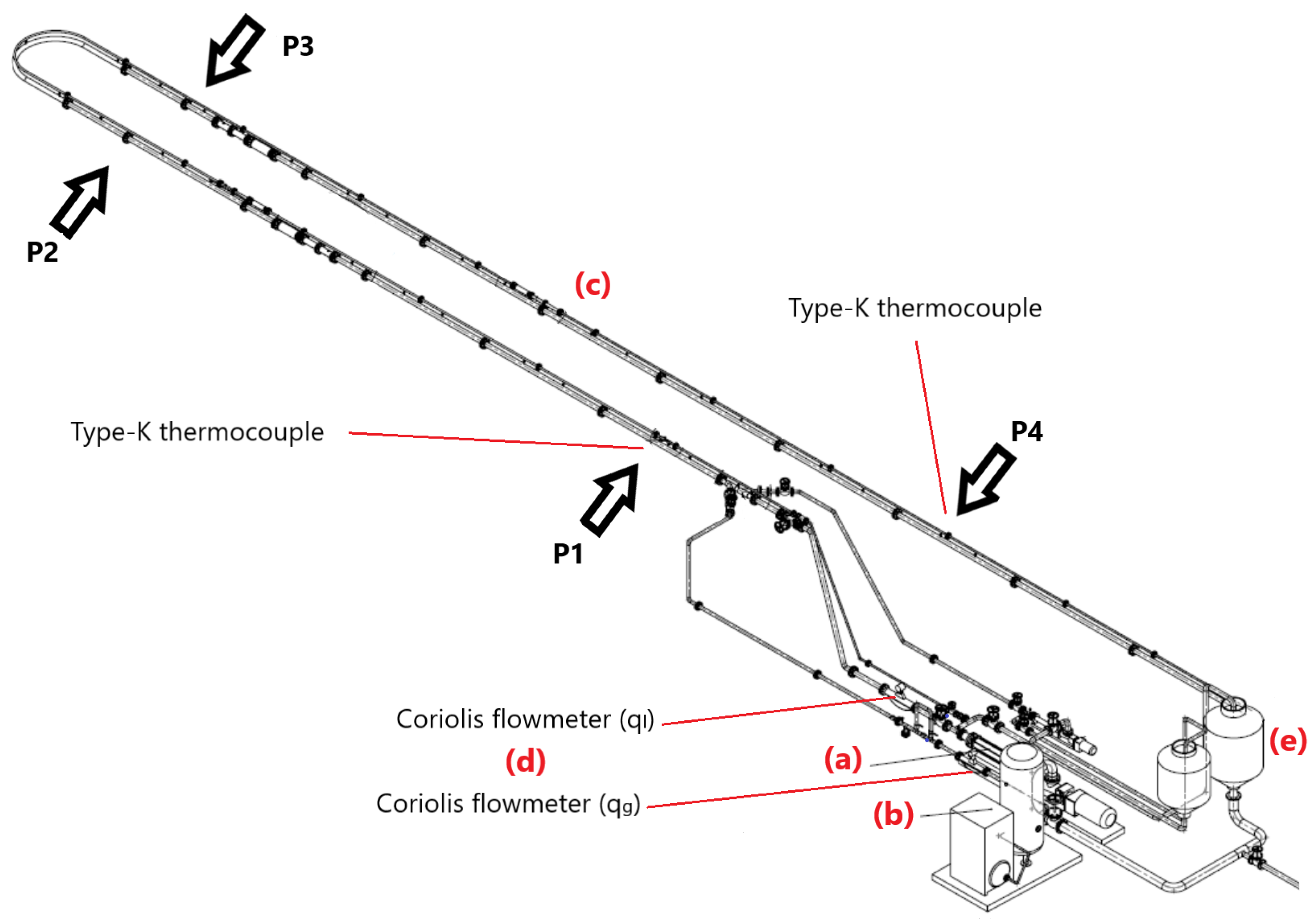
2.1. Test Apparatus
2.2. Methodology
3. Results and Discussion
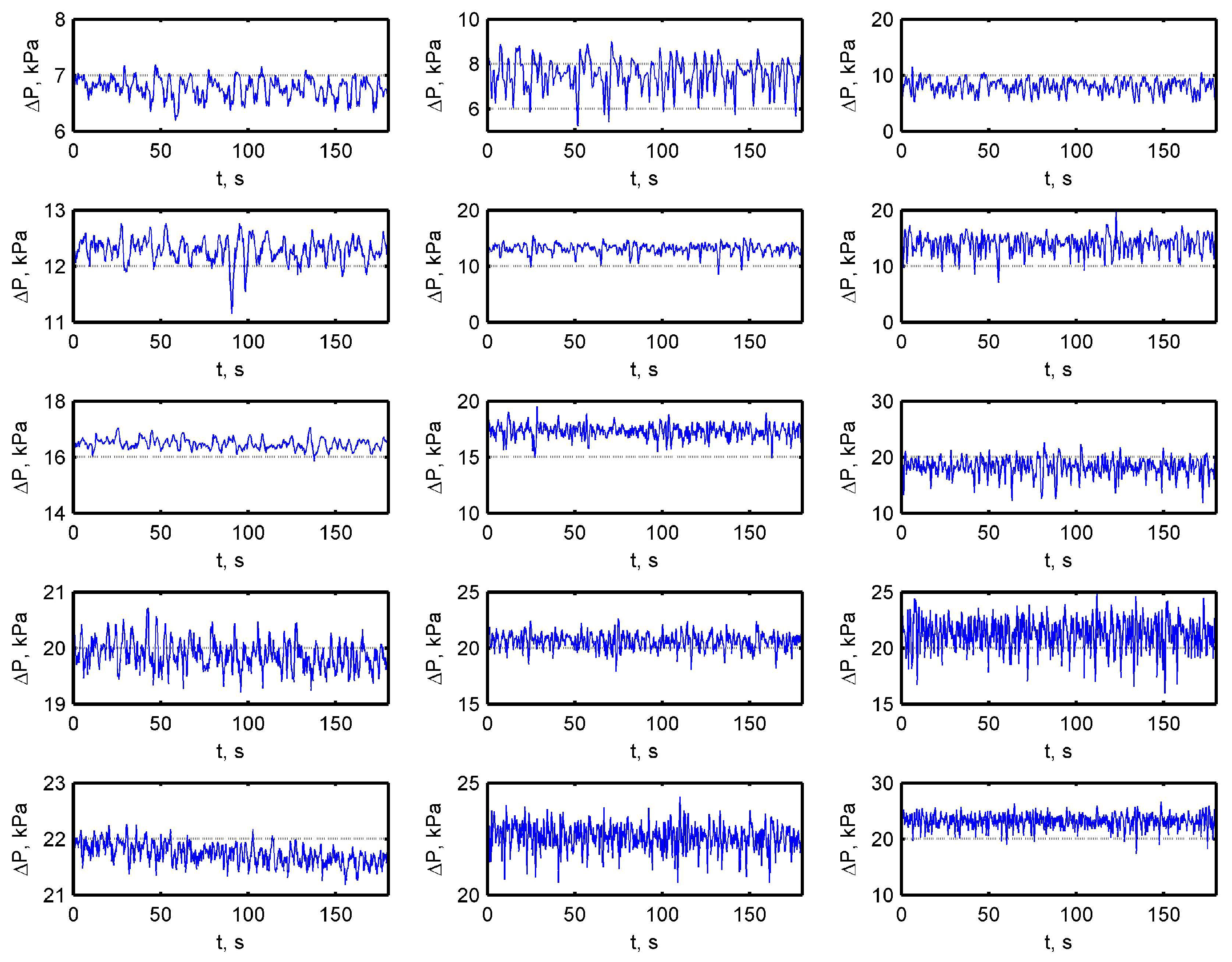
3.1. Pressure Response
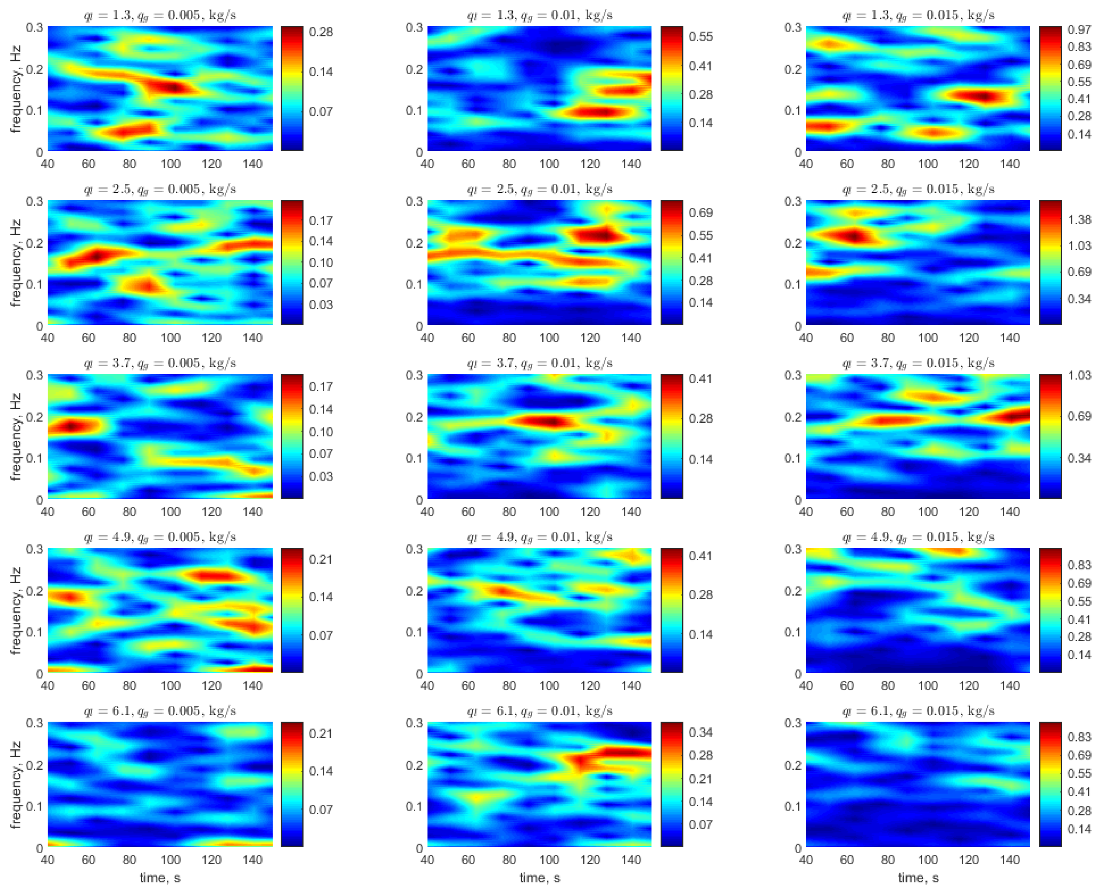
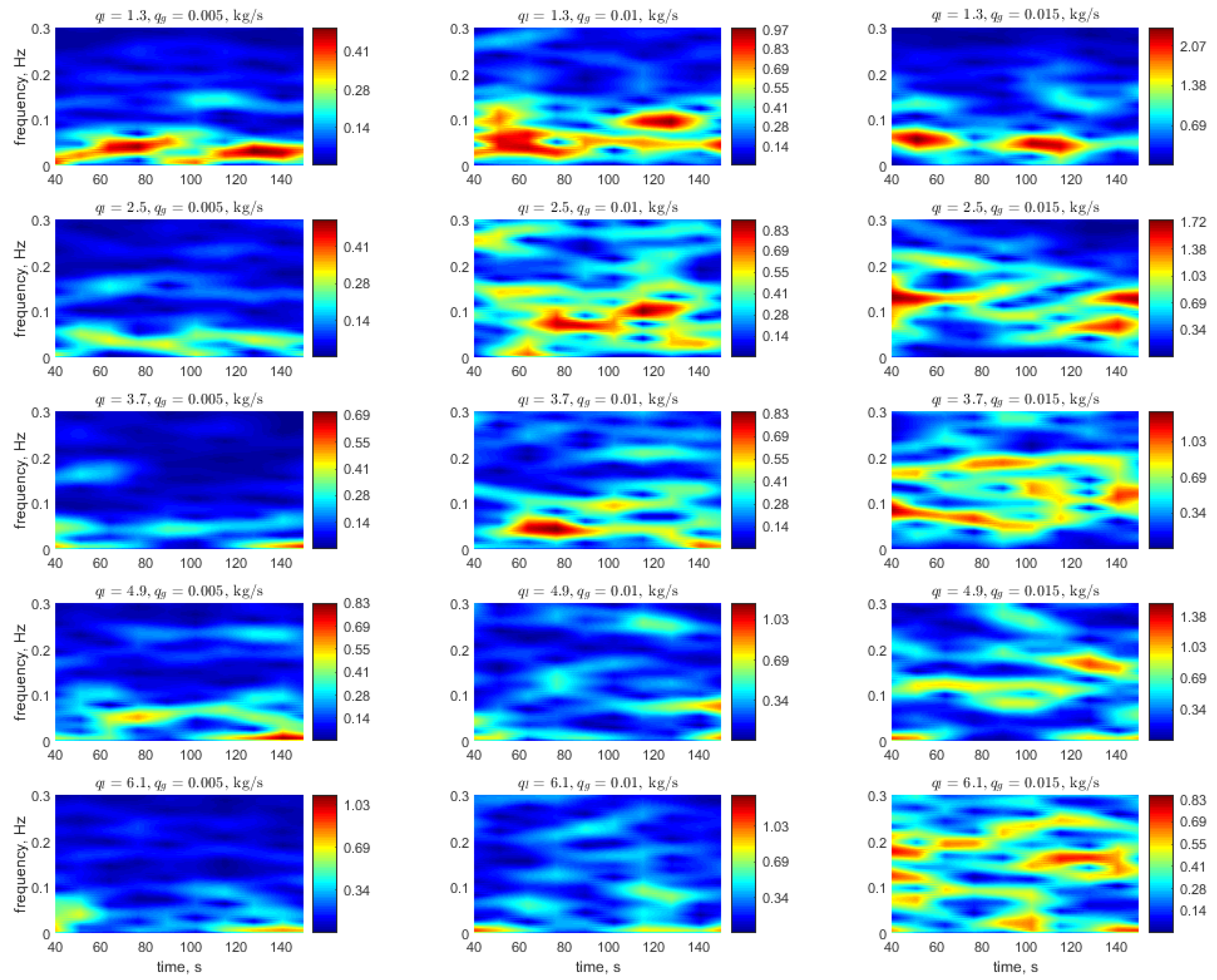
3.2. Spectral Evolution of the Flow
3.3. Detrended Fluctuation Analysis (DFA)
- : The fluctuations are anti-correlated.
- : The fluctuations are uncorrelated and represent noise; i.e., white noise.
- : The fluctuations have positive autocorrelation.
- : The fluctuations represent noise; i.e., pink noise.
- : The fluctuations are non-stationary.
- : The fluctuations represent noise; i.e., Brownian noise.
- The pressure drop exhibits a space-wise evolution. It may be caused by local variations of the phase volume fractions, which take place as the mixture evolves downstream along the pipe. For example, consider the flow produced with (0.005 kg/s, 1.3 kg/s) (upper most squares of columns 1, 4 and 7 of the table). The pressures appear to be autocorrelated except at the downstream section.In other words, the pressure measured at P1 corresponds to the pressures measured at P2 and P3, the three being in-phase because (positive autocorrelation). On the downstream section, however, the pressure measured at P4 does not correspond to any of the measurements at P1, P2 or P3. Hence, three possibilities arise: a) the coherence may be lost to the strong effects induced by the ejection of irregular liquid lumps at the outlet, b) secondary flows at the U-turn may have a disruptive effect on the properties of the pressure waves, and c) a combination of the two. The reason for these possibilities is that the U-turn and the outlet are the only two points in the flow system where the two following effects can take place: secondary flows due to the centripetal acceleration undergone by the flow inside the U-turn section, and the sudden depressurization caused by the ejection of the liquid slugs into the separator tank.
- Apparently, very few flows exhibit white noise characteristics or non-stationary fluctuations. The former are more related with higher liquid and gas flow rates, while the latter are more related with low and high liquid .The non-stationary cases represented by are interesting, because they indicate that the mean values of the pressures are varying with time (or equivalently with position). Even though these variations might be slight, the method is still capable of identifying them. This opens up the prospect of designing techniques for industrial applications. Obvious examples would be the development of methods to detect small leakages in pipelines, or to detect slow corrosion processes.
- It is worth noticing that pink noise processes are mostly observed at the outlet section of the pipe. In general, the values of this section appear to show a relative increase with respect to the values of the inlet section. This suggests that the scaling exponent increases in the direction of the flow.Since pink noise refers to scalability, the reproduction of self-similar patterns and small scale traits of the signal would suggest the existence of an energy distribution process (analogous to the energy cascade in turbulence). However, it is noted that only the cases corresponding to the inlet flow rates (0.005 kg/s, 4.9 kg/s) and (0.01 kg/s, 6.1 kg/s) maintain this behavior. On the other hand, only the flow combination (0.005 kg/s, 6.1 kg/s) seems to correspond to this process in the U-turn. Overall, from the physical point of view, these characteristics would be mostly related with the ejection effects produced at the outlet of the pipe.
- Interestingly, not a single combination of inlet gas–liquid flow rates produced fully random processes in this kind of flow system. The question still remains whether such Brownian noise patterns would eventually emerge in a longer pipeline, or not. The same question could be asked regarding the flow rates.Anti-correlated flows for which seem to dominate in the U-turn section of the pipe. This is particularly true with high flow regimes, that is, those produced with elevated inlet mass flow rates. Similar anti-correlations are also observed at the inlet and outlet section of the pipe with high flow rates. These cases indicate that the phases of the pressure waves shift by approximately radians, as they progress from one pressure port to the next one.
4. Conclusions
Author Contributions
Funding
Acknowledgments
Conflicts of Interest
Nomenclature
| d | diameter | (m) |
| f | frequency | (Hz) |
| l | length | (m) |
| p | pressure | (kPa) |
| q | flow rate | (m/s) |
| t | time | (s) |
| u | velocity | (m/s) |
| x | length | (m) |
| pressure profile | (kPa) | |
| scaling exponent | - | |
| standard deviation | (kPa) | |
| dynamic viscosity | (Pa·s) | |
| density | (kg/m) | |
| Re | Reynolds number | - |
| avg | average | |
| l | liquid | |
| g | gas | |
| i, k, n | dummy indices | |
| N | number of data points |
References
- Hart, A. A review of technologies for transporting heavy crude oil and bitumen via pipelines. J. Pet. Explor. Prod. Technol. 2013, 4, 1–10. [Google Scholar] [CrossRef]
- Matsubara, H.; Naito, K. Effect of Liquid Viscosity on Flow Patterns of Gas-Liquid Two-Phase Flow in a Horizontal Pipe. Int. J. Multiph. Flow 2011, 37, 1277–1281. [Google Scholar] [CrossRef]
- Hernandez, J.; Montiel, J.C.; Palacio-Perez, A.; Rodríguez-Valdés, A.; Guzmán, J.E.V. Horizontal Evolution of Intermittent Gas-Liquid Flows With Highly Viscous Phases. Int. J. Comput. Methods Exp. Meas. 2018, 6, 152–161. [Google Scholar]
- Foletti, C.; Farisé, S.; Grassi, B.; Strazza, D.; Lancini, M.; Poesio, P. Experimental investigation on two-phase air/high-viscosity-oil flow in a horizontal pipe. Chem. Eng. Sci. 2011, 66, 5968–5975. [Google Scholar] [CrossRef]
- Khaledi, H.A.; Smith, I.E.; Unander, T.E.; Nossen, J. Investigation of two-phase flow pattern, liquid holdup and pressure drop in viscous oil–gas flow. Int. J. Multiph. Flow 2014, 67, 37–51. [Google Scholar] [CrossRef]
- Zhao, Y.; Yeung, H.; Zorgani, E.E.; Archibong, A.E.; Lao, L. High viscosity effects on characteristics of oil and gas two-phase flow in horizontal pipes. Chem. Eng. Sci. 2013, 95, 343–352. [Google Scholar] [CrossRef]
- Zhao, Y.; Lao, L.; Yeung, H. Investigation and prediction of slug flow characteristics in highly viscous liquid and gas flows in horizontal pipes. Chem. Eng. Res. Des. 2015, 102, 124–137. [Google Scholar] [CrossRef] [Green Version]
- Al-Safran, E.; Kora, C.; Sarica, C. Predictiono of slug liquid holdup in high-viscosity liquid and gas two-phase flow in horizontal pipes. J. Pet. Sci. Eng. 2015, 133, 566–575. [Google Scholar] [CrossRef]
- Farsetti, S.; Farisé, S.; Poesio, P. Experimental investigation of high-viscosity oil-air intermittent flow. Exp. Therm. Fluid Sci. 2014, 57, 285–292. [Google Scholar] [CrossRef]
- Gokcal, B.; Al-sarki, A.M.; Sarica, C.; Al-Safran, E.M. Prediction of slug frequency for high-viscosity oils in horizontal pipes. SPE Proj. Facil. Constr. 2009, 124057, 447–461. [Google Scholar]
- Okezue, C.N. Application of the gamma radiation method in analysing the effect of liquid viscosity and flow variables on slug frequency in high-viscosity oil–gas horizontal flow. Comput. Methods Multiph. Flow VII 2007, 79, 447–461. [Google Scholar]
- Baba, Y.D.; Archibong, A.E.; Aliyu, A.M.; Ameen, A.I. Slug frequency in high-viscosity oil–gas two-phase flow: Experiment and prediction. Flow Meas. Instrum. 2017, 54, 109–123. [Google Scholar] [CrossRef]
- Losi, G.; Arnone, D.; Correra, S.; Poesio, P. Modelling and statistical analysis of high-viscosity oil/air slug flow characteristics in a small diameter horizontal pipe. Chem. Eng. Sci. 2016, 148, 190–202. [Google Scholar] [CrossRef]
- Zahi, L.S.; Jin, N.D.; GAo, Z.K.; Chen, P.; Chi, H. Gas-Liquid Two Phase Flow Pattern Evolution Characteristics Based on Detrended Fluctuation Analysis. J. Metrol. Soc. India 2011, 26, 255–265. [Google Scholar]
- Peng, C.K.; Buldyrev, S.V.; Havlin, S.; Simons, M.; Stanley, H.E.; Goldberger, A.L. Mosaic organization of DNA nucleotides. Phys. Rev. E 1994, 49, 1685. [Google Scholar] [CrossRef]
- Kantelhardt, J.W.; Koscielny-Bunde, E.; Rego, H.H.; Havlin, S.; Bunde, A. Detecting long-range correlations with detrended fluctuation analysis. Phys. A Stat. Mech. Its Appl. 2001, 295, 441–454. [Google Scholar] [CrossRef] [Green Version]
- Subhakar, D.; Chandrasekhar, E. Reservoir characterization using multifractal detrended fluctuation analysis of geophysical well-log data. Physica A 2016, 445, 57–65. [Google Scholar] [CrossRef]
- Ribeiro, R.A.; Mata, M.V.M.; Lucena, L.S.; Corso, G. Spatial analysis of oil reservoirs using detrended fluctuation analysis of geophysical data. Nonlinear Process. Geophys. 2014, 21, 1043–1049. [Google Scholar] [CrossRef] [Green Version]
- Moffat, R.J. Contributions to the Theory of Single-Sample Uncertainty Analysis. Trans. ASME 1982, 104, 250–258. [Google Scholar] [CrossRef] [Green Version]
- Holman, J.P. Experimental Methods for Engineers, 6th ed.; McGraw-Hill: New York, NY, USA, 1994. [Google Scholar]
- Tompkins, C.; Prasser, H.M.; Corradini, M. Wire-mesh sensors: A review of methods and uncertainty in multiphase flows relative to other measurement techniques. Nucl. Eng. Des. 2018, 337, 205–220. [Google Scholar] [CrossRef]
- Ameran, H.L.M.; Mohamad, E.J.; Muji, S.Z.; RAhim, R.A.; Abdullah, J.; Rashid, W.N.A. Multiphase flow velocity measurement of chemical processes using electrical tomography: A review. In Proceedings of the IEEE 2016 International Conference on Automatic Control and Intelligent Systems (I2CACIS), Bandar Hilir, Malaysia, 16–18 December 2016; pp. 162–167. [Google Scholar]
- Arvoh, B.K.; Hoffmann, R.; Halstensen, M. Estimation of volume fractions and flow regime identification in multiphase flow based on gamma measurements and multivariate calibration. Flow Meas. Instrum. 2012, 23, 56–65. [Google Scholar] [CrossRef]
- Hanafizadeh, P.; Eshraghi, J.; Taklifi, A.; Ghanbarzadeh, S. Experimental identification of flow regimes in gas–liquid two phase flow in a vertical pipe. Meccanica 2016, 51, 1771–1782. [Google Scholar] [CrossRef]
- Matsui, G. Identification of flow regimes in vertical gas–liquid two-phase flow using differential pressure fluctuations. Int. J. Multiph. Flow 1984, 10, 711–719. [Google Scholar] [CrossRef]


| Fluid | Viscosity (Pa·s) | Density (kg/m) | Interfacial Tension (N/m) |
|---|---|---|---|
| Air | 1.8 | 1.2 | - |
| Glycerine | 1.1 | 1.2 × 10 | 6.3 × 10 |
| (kg/s) | (kg/s) |
|---|---|
| 1.3 | |
| 0.005 | 2.5 |
| 0.01 | 3.7 |
| 0.015 | 4.9 |
| 6.1 |
| - | 0.005 | 0.01 | 0.015 | 0.005 | 0.01 | 0.015 | 0.005 | 0.01 | 0.015 |
| 1.3 | 0.72 | 0.43 | 0.37 | 0.67 | 0.27 | 0.34 | 0.94 | 0.52 | 0.63 |
| 2.5 | 0.84 | 0.37 | 0.27 | 0.79 | 0.19 | 0.22 | 0.99 | 0.62 | 0.42 |
| 3.7 | 1.15 | 0.75 | 0.45 | 0.77 | 0.41 | 0.24 | 1.11 | 0.63 | 0.33 |
| 4.9 | 1.03 | 0.88 | 0.68 | 0.82 | 0.46 | 0.33 | 1.02 | 0.97 | 0.86 |
| 6.1 | 1.18 | 1.03 | 0.78 | 1.04 | 0.69 | 0.51 | 1.08 | 1.05 | 0.78 |
© 2019 by the authors. Licensee MDPI, Basel, Switzerland. This article is an open access article distributed under the terms and conditions of the Creative Commons Attribution (CC BY) license (http://creativecommons.org/licenses/by/4.0/).
Share and Cite
Hernández, J.; Galaviz, D.F.; Torres, L.; Palacio-Pérez, A.; Rodríguez-Valdés, A.; Guzmán, J.E.V. Evolution of High-Viscosity Gas–Liquid Flows as Viewed Through a Detrended Fluctuation Characterization. Processes 2019, 7, 822. https://doi.org/10.3390/pr7110822
Hernández J, Galaviz DF, Torres L, Palacio-Pérez A, Rodríguez-Valdés A, Guzmán JEV. Evolution of High-Viscosity Gas–Liquid Flows as Viewed Through a Detrended Fluctuation Characterization. Processes. 2019; 7(11):822. https://doi.org/10.3390/pr7110822
Chicago/Turabian StyleHernández, J., D. F. Galaviz, L. Torres, A. Palacio-Pérez, A. Rodríguez-Valdés, and J. E. V. Guzmán. 2019. "Evolution of High-Viscosity Gas–Liquid Flows as Viewed Through a Detrended Fluctuation Characterization" Processes 7, no. 11: 822. https://doi.org/10.3390/pr7110822