Interactive Tool for Frequency Domain Tuning of PID Controllers


1
Department of Computer Science and Numerical Analysis, University of Cordoba, Campus de Rabanales, 14071 Cordoba, Spain
2
Department of Mechanical Engineering, University of Cordoba, Campus de Rabanales, 14071 Cordoba, Spain
3
Department of Computer Science and Automatic Control, National Distance Education University, 28040 Madrid, Spain
*
Author to whom correspondence should be addressed.
Processes 2018, 6(10), 197; https://doi.org/10.3390/pr6100197
Submission received: 25 September 2018
/
Revised: 15 October 2018
/
Accepted: 16 October 2018
/
Published: 18 October 2018
(This article belongs to the Section Advanced Digital and Other Processes)
Abstract
:This paper presents an interactive tool focused on the study of proportional-integral-derivative (PID) controllers. Nowadays, PID control loops are extensively used in industrial applications. However, it is reported that many of them are badly tuned. From an educational point of view, it is essential for undergraduate students in control engineering to understand the importance of tuning a control loop correctly. For this reason, the tool provides different PID tuning methods in the frequency domain for stable open-loop time-delay-free processes. The different designs can be compared interactively by the user, allowing them to understand concepts about stability, robustness, and performance in PID control loops. A survey and a comparative study were performed to evaluate the effectiveness of the proposed tool.
1. Introduction
Research and development activities regarding engineering education, and especially about control engineering, have been receiving growing attention during recent years. Proportional-integral-derivative (PID) controllers have widespread acceptance in most industrial applications due to their simple structure, satisfactory control effect, and acceptable robustness [1,2]. According to Reference [3], PID controls represent more than 95% of the controllers in process control applications, and particularly, about 98% of control loops are controlled by PID controllers in the pulp and paper industries [4]. Although it is a traditional type of controller in use since the mid-20th century, one of the conclusions reached at the IFAC Conference on Advances in PID control, held in Brescia (Italy) in 2012, was that PID controllers will stay as the preferred control algorithms at the bottom layer in spite of other promising proposals, such as model predictive control paradigms [5].
Nevertheless, several surveys show that there is still poor communication of the academic work to the industrial community. For instance, in Reference [6] it is reported that 80% of PID controllers are badly tuned, 30% of them operate in manual mode, and about 25% of all PID control loops use default factory settings. Therefore, it is important there is an improvement in education and training on tuning these kinds of controllers. There are hundreds, if not thousands, of works that have been written on PID controller tuning methods and rules [7,8]. Since Ziegler and Nichols (1942) presented their PID controller tuning rules [9], several approaches have been developed. Some methods are model-based techniques, such as tuning rules for minimizing some performance criteria based on an integrated error criterion [10], achieving some robustness specification [11], or obtaining a specified closed-loop response using time-domain metrics [12]. Other methods propose a tradeoff between performance and robustness, or between servo and regulation modes [13,14]. However, most of these methodologies are usually based on a simple model of the dynamics of the process, and a previous model reduction is necessary. Other methodologies based on the frequency response allow PID design for any arbitrary order irrational or non-minimum phase stable transfer functions [3,15]. These methods use robustness conditions in the frequency domain, such as phase margin, gain margin, maximum sensitivity, and so on [16].
This work reports the design and application of an interactive Matlab-based tool focused on tuning and simulation of single input single output (SISO) PID controllers for stable processes without time delay. The objective is the application and teaching of PID tuning methods based on frequency response specifications supported by a graphical interpretation. The proposed tool has been developed using the basic features of Matlab 2012b (MathWorks, Natick, MA, USA) [17] without adding extra toolboxes, and provides a set of PID tuning methodologies in the frequency domain for stable processes. Although there is a growing trend regarding the exploitation of open source tools for educational purposes, the reliability and widespread use of the Matlab suite in the academic world can be pointed to as one of its main benefits. Interactive software for teaching control is supported for several reasons [18,19,20,21,22]: (a) Learning efficiency can be increased by using computer aided design and analysis tools; (b) modifying properties and instantaneously observing the corresponding effects is very helpful both for design and learning processes; (c) these tools support the combination between theory and practice contents; (d) the interactive comparison of designs based on different frequency domain specifications allows one to understand fundamental ideas about stability, robustness, and performance in PID control loops.
An initial version of the tool was presented in a conference article [16]. In the current work, the tool has been applied for educational purposes, and has been improved and increased, also taking into account practical considerations, such as simulation with a controller discrete implementation, sample time modification, and process input saturations. This makes the tool not only interesting for control engineering education, but also to be used by operators in real cases. The tool is available at http://www.dia.uned.es/~fmorilla/Herramientas/pidgui.zip.
This paper is organized as follows: The PID tuning methodologies implemented in the tool are explained in Section 2. Section 3 and Section 4 give a detailed description of the use of the tool, providing an illustrative example. Finally, a tool evaluation is provided in Section 5, describing the corresponding educational experience. Conclusions are summarized in Section 6.
2. Tuning of PID Controllers in the Frequency Domain
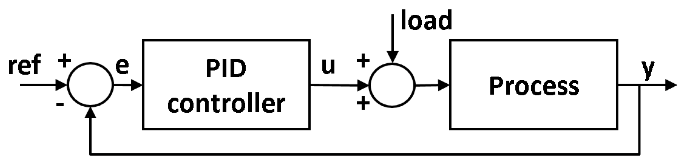
In this work, the feedback control system shown in Figure 1 is assumed. The signal y is the controlled variable, ref is the reference signal, u is the control signal, and load is an input disturbance.
The plant model is a rational transfer function P(s) given by Equation (1), where the roots of the denominator A(s) are not in the right half-plane. The PID controller C(s) is given by Equation (2), where KP is the proportional gain, KI the integral gain (thus, the integral time constant TI equals KP/KI), and KD is the derivative gain (thus, the derivative time constant TD equals KD/KP).
P(s) = B(s)/A(s)
C(s) = KP + KI/s + KD·s
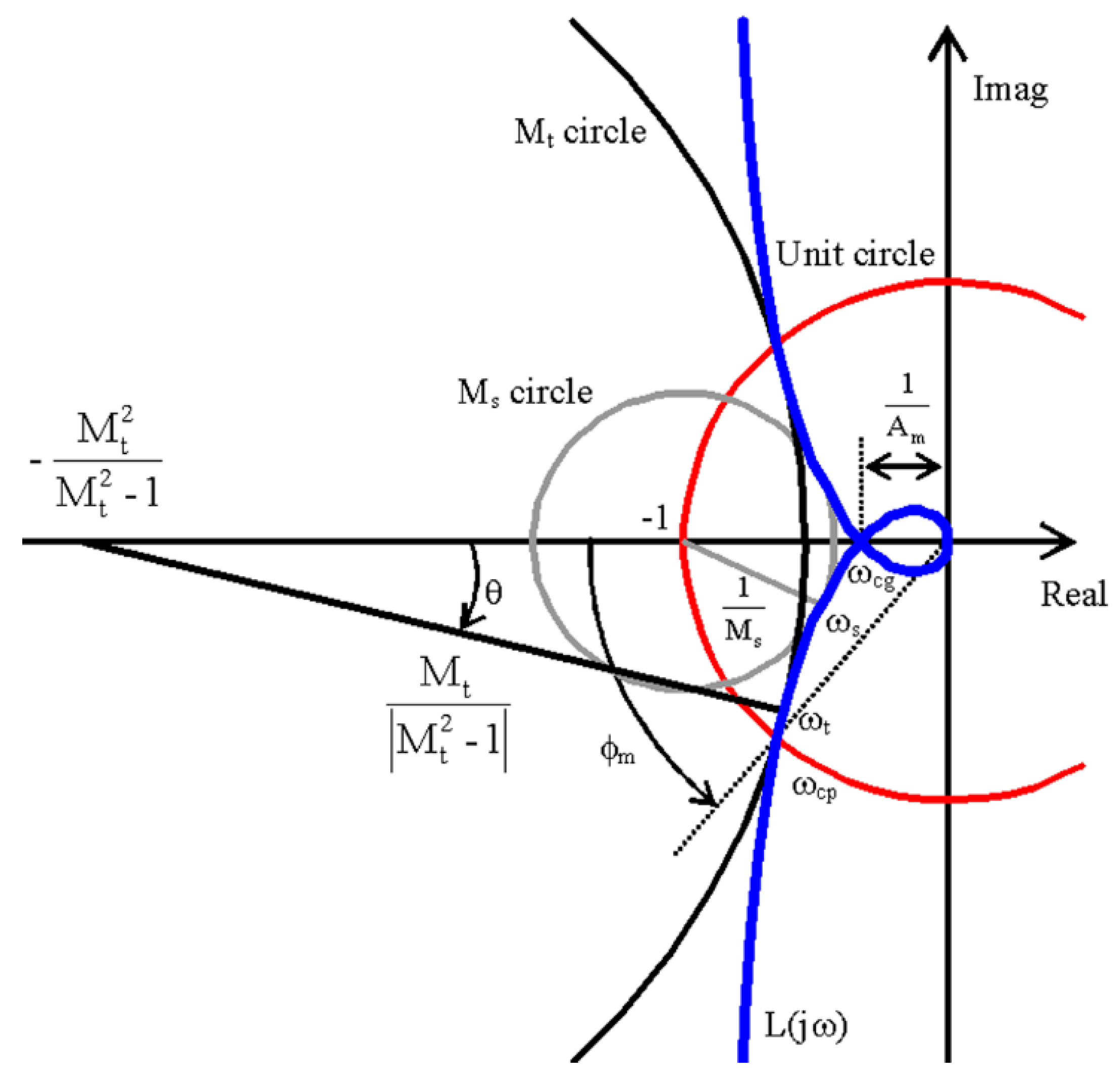
In PID control design, in addition to closed loop stability, it is common to specify some quantitative measures of “how far from instability” the nominal loop is. In this work, four robustness conditions are considered: Maximum sensitivity Ms, maximum complementary sensitivity Mt, phase margin ϕm, and gain margin Am. They are represented in Figure 2. The gain margin indicates how much the controller gain can be increased before reaching the stability limit, and it is calculated using the smallest frequency (ωcg), where the phase lag of the open-loop transfer function is 180°. The phase margin is the phase lag required to reach the stability limit at the frequency ωcp, where the Nyquist plot intersects the unit circle. Both gain and phase margins are classical measures of relative stability, and both margins must be positive to assure stability for stable open-loop processes. The maximum sensitivity Ms is the reciprocal to the radius of the circle with center in point −1 and tangent to the Nyquist plot at ωs, so it measures the shortest distance to the critical point −1. Similarly, the maximum complementary sensitivity Mt is related to the shortest distance from the Nyquist curve to another circle with it’s center at a negative real axis point and enclosing the critical point −1. The requirements that maximum sensitivity and complementary sensitivity are less than Ms and Mt, respectively, imply that the Nyquist plot must be outside the corresponding circles [3].
These specifications provide a set of acceptable values of the controller parameters describing the boundary curves for the corresponding frequency domain requirements in the parameter plane KP-KI or KP-KD [23]. However, it is also necessary to guarantee the closed-loop stability in the PID controller design, which involves a boundary stability region in the same controller parameter spaces. The next subsections explain the calculation of the stability regions and the frequency requirement boundary curves for five types of PID controllers.
2.1. Stability Regions
The PID controller must be tuned to achieve a stable closed-loop response with some additional specifications. Given a particular process Equation (1), the set of controller parameters that stabilizes the feedback system in Figure 1 is called the stability region. It can be analytically determined as a bounded region in the controller parameter space. Given the feedback control system of Figure 1, the characteristic equation of the closed-loop system f(s; KP, KI, KD) is given by:
s·A(s) + s2·KD·B(s) + s·KP·B(s) + KI·B(s) = 0.
Since there are three parameters, the stability region of this family is a subset of R3. Being A(s) and B(s) polynomials, the family of polynomials compounding the characteristic Equation (3) is called a polytope [24], and it can be comprised of several disjoint sets. According to Reference [25], the stability region can be obtained in terms of the parametric space achieving necessary and sufficient conditions. Then, low cost computations allow for calculating the stability region in the plane. With three parameters it is necessary to scan along one of them, and this implies an increase of the computational cost. In this work, only two controller parameters are considered for calculating the stability region; the third one is fixed in some way. Therefore, the stability region is represented in a R2 parameter plane. Five cases are considered:
- PI: Where KD = 0.
- PD: Where KI = 0.
- PIDα: Where the ratio of the derivative and integral time constants α = TD/TI remains constant. This is equal to fix KD = α·(KP)2/KI.
- PIDKD: Where KD is set to a fixed value.
- PIDKI: Where KI is set to a fixed value.
Table 1 shows the parameter plane for each case and the corresponding characteristic equation, where:
AD(s) = A(s) + s·KD·B(s); BD(s) = B(s);
AI(s) = s·A(s) + KI·B(s); BI(s) = s·B(s).
AI(s) = s·A(s) + KI·B(s); BI(s) = s·B(s).
Figure 3 shows an example of the stability region in the KP-KI parameter plane for a non-minimum phase process described by the transfer function Equation (5). This gray area is calculated for the PIDα control with α = 0.1.
The notation of Table 1 allows the PIDKD control to include the PI control as a particular case when KD = 0. In a similar way, the PD control is also included as a special case of the PIDKI control when KI = 0. The process transfer function in Equation (1) does not include time delay in order to determine the stability regions accurately.
2.2. Specification Boundary Curves
Some frequency domain PID tuning methods can be interpreted in terms of moving one point A in the frequency response of the process P(jω) to an arbitrary point B of the Nyquist plot L(jω) = C(jω)·P(jω) [26]. This point B is determined by the frequency specification: Gain margin (GM), phase margin (PM), maximum sensitivity (Ms), and maximum complementary sensitivity (Mt). Table 2 defines the corresponding target points B for the four specifications. It is determined by the magnitude rB and the phase ϕB with respect to the origin and to the negative real axis. In the sensitivity specifications, R and c are the radius and the center of the respective circle. The angle θ is the angle of the radius where the Nyquist plot tangentially contacts the respective circle and the negative real axis.
These specifications provide a subset of R3 given by all possible 3-tuples of gains (KP, KI, KD) fulfilling the conditions (6) and (7), where r(ω) and ϕ(ω) are the magnitude and the phase of P(jω), respectively, with respect to the origin and the negative real axis.
Thus, some point A (r(ωd), ϕ(ωd)) at the design frequency ωd of the process Nyquist plot Equation (8) is mapped to the target point B (rB, ϕB) of the loop Nyquist plot Equation (9).
P(jω) = r(ω) × ej(ϕ(ω)−180°)
L(jω) = C(jω) × P(jω) = (KP − jKI/ω + jωKD) × P(jω)
Equation (7) is particularized in Table 3 for the different cases where some additional requirement is imposed on the controller gains to have only two free parameters as was mentioned in the previous section. In this manner, the subset of controllers fulfilling the specifications can be represented as a boundary curve in the respective parameter plane KP-KI or KP-KD. The special cases of PI and PD control are also included in the second and third rows of Table 3, respectively, when KD = 0 for PI control and KI = 0 for PD control. It is possible that part of the boundary curve lies outside the corresponding stability region. This part of the curve is not admissible for selecting the controller parameters. Figure 3 also shows in blue an example of a boundary curve of phase margin of 60° obtained for process Equation (5) and the PIDα control. The stabilizing region is divided by this curve into two zones: I (ϕm > 60°) and II (ϕm < 60°). Tuning the controller parameters is easy with this information. If a phase margin ϕm = 60° is desired, a point of the boundary curve must be selected. It is usually advisable to select the point with the maximum KI [26] to improve the disturbance rejection performance. For ϕm > 60°, a point inside zone I is acceptable, and any point of zone II obtains ϕm < 60°. Any point close to the stability boundary is not recommendable.
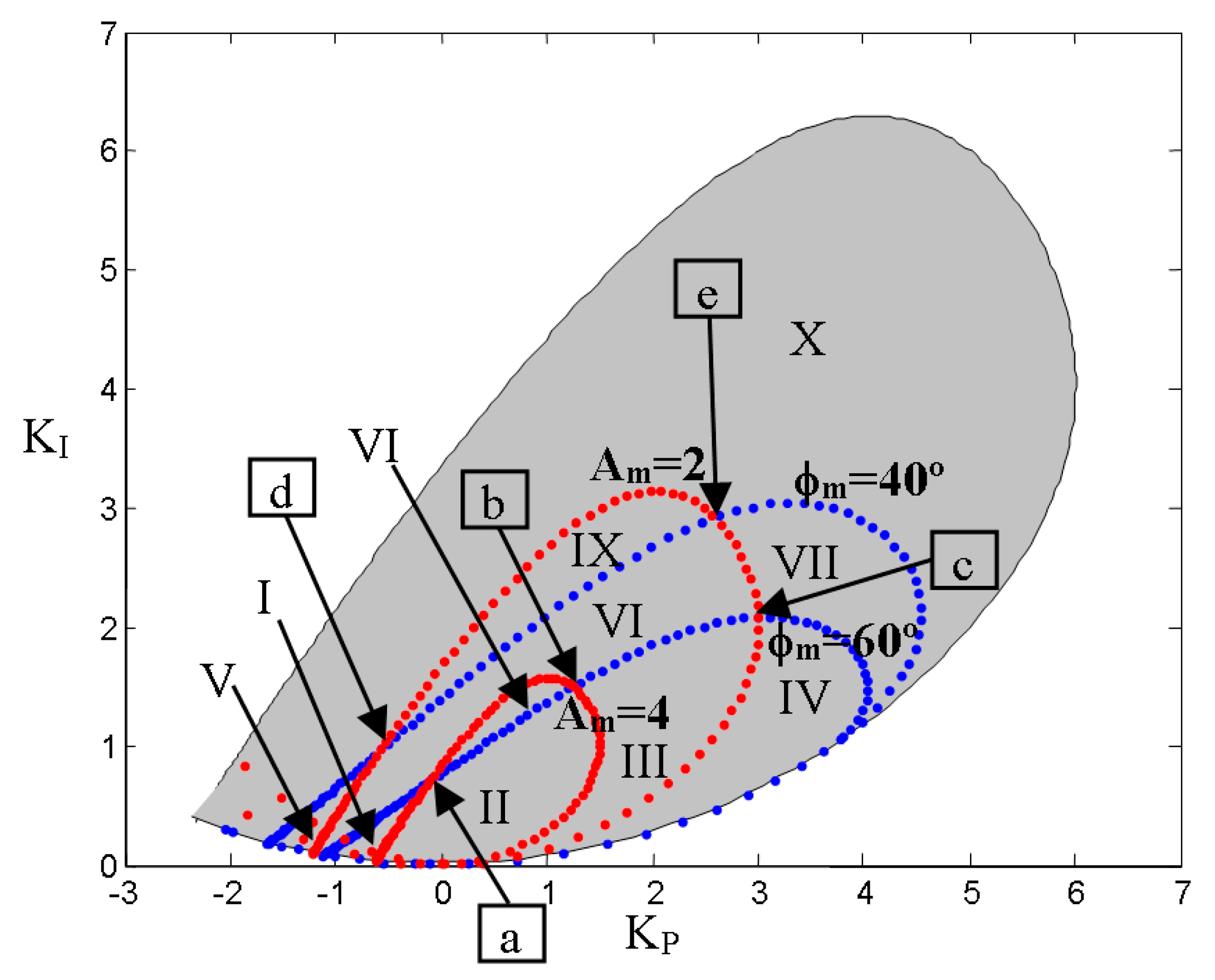
In addition, when different requirements or two values of the same specifications are combined, it is possible to obtain useful information. For the non-minimum process in Equation (5) and the PIDα control, Figure 4 shows how four boundary curves (ϕm = 60°, ϕm = 40°, Am = 4, and Am = 2) split the stabilizing region into ten zones (from I to X), highlighting five interesting points (from a to e) where two different boundary curves intersect. The achieved specifications in these zones and points are the following:
- Zone I: ϕm = 60°, 2 ≤ Am ≤ 4
- Zone II: ϕm = 60°, Am = 4
- Zone III: ϕm = 60°, 2 ≤ Am ≤ 4
- Zone IV: ϕm = 60°, Am ≤ 2
- Zone V: 40° ≤ ϕm ≤ 60°, Am ≤ 2
- Zone VI: 40° ≤ ϕm ≤ 60°, 2 ≤ Am ≤ 4
- Zone VII: 40° ≤ ϕm ≤ 60°, Am = 4
- Zone VIII: 40° ≤ ϕm ≤ 60°, Am ≤ 2
- Zone IX: ϕm ≤ 40°, 2 ≤ Am ≤ 4
- Zone X: ϕm ≤ 40°, Am ≤ 2
- Point a: ϕm = 60°, Am = 4
- Point b: ϕm = 60°, Am = 4
- Point c: ϕm = 60°, Am = 2
- Point d: ϕm = 40°, Am = 2
- Point e: ϕm = 40°, Am = 2
When Ms or Mt are used as frequency domain specifications, it is preferable to calculate the boundary curve for a range of values of θ (for instance, from 5° to 45°) instead of a single value. Furthermore, it is necessary to verify the tangency condition at the target point B [26]. This condition is summarized in Equation (10), where r’B(ω) and ϕ’B(ω) are values of the magnitude and phase derivatives of L(jω) at the point B, respectively.
Consequently, estimating the Ms and Mt boundary curves implies more calculations than estimating the curves for ϕm and Am. For the process in Equation (5) and the PIDα control, Figure 5 shows an example where the stabilizing region is divided into three zones by the boundary curves Ms = 1.8 and Mt =1.6: I (Ms ≤ 1.8, Mt ≤ 1.6), II (Ms = 1.8, Mt ≤ 1.6), and III (Ms = 1.8, Mt = 1.6).
The closed-loop response of the feedback system in Figure 1 is different for each frequency domain specification. Thanks to the proposed tool, it is possible to compare different controllers achieving different frequency requirements (or the same specification at different frequencies), and thus analyze the corresponding effect in the time response of the controlled variable and control signal.
2.3. Discrete Implementation and Practical Considerations
Most of the PID methodologies for process control in literature are developed assuming a continuous controller implementation. Nevertheless, real controllers are discrete in practice. Therefore, it is necessary to implement or configure the controller with a proper sample time. Usually, the typical sample time is very small in comparison with the typical process dynamics in many industrial applications, and consequently, no considerations are needed. However, for applications with fast dynamics, a bad choice of the controller sample time can deteriorate the closed-loop response, and can even turn it unstable.
In the developed tool, simulations are performed using a discrete implementation of the controller, and thus the effects of the sample time modification can be analyzed. Specifically, the discrete implementation is based on the Tustin approximation [3]. Then, the control signal in the k sample time u(k) is calculated according to the control block of the discrete PID algorithm described in Table 4, where P(k) is the proportional action of the control signal, I(k) is the integral one, D(k) is the derivative one, and h is the sample time. The “k-1” elements are the ones corresponding to the previous sample time, and they are initially set to zero.
The coefficients a and b multiplying the set-point in the proportional action and the derivative action, respectively, can be used to implement the PID controller as the called PI-D and I-PD control strategies, when b or a, and b, are fixed to 0. These structures avoid the derivative and proportional kick effects, that cause large control signal values when there is a sudden step change in the reference, and the proportional or derivative gains are high [3]. Furthermore, another important practical aspect to take into account in a real process is the upper and lower limitations of the process input (umax and umin). In fact, the undesired windup effect can arise in control strategies with integral action, such as PID or PI control, when some control signal constraint is reached. The tool is prepared to configure limits in the control signal, and an anti-windup mechanism is implemented in the PID controller to avoid the windup effect. This strategy is shown in the anti-windup block of Table 4. If the initially calculated control signal is out of range, the current integral action I(k) is updated and limited in such a way that the new sum of P(k), I(k), and D(k) is within the validity range.
3. Graphical User Interface
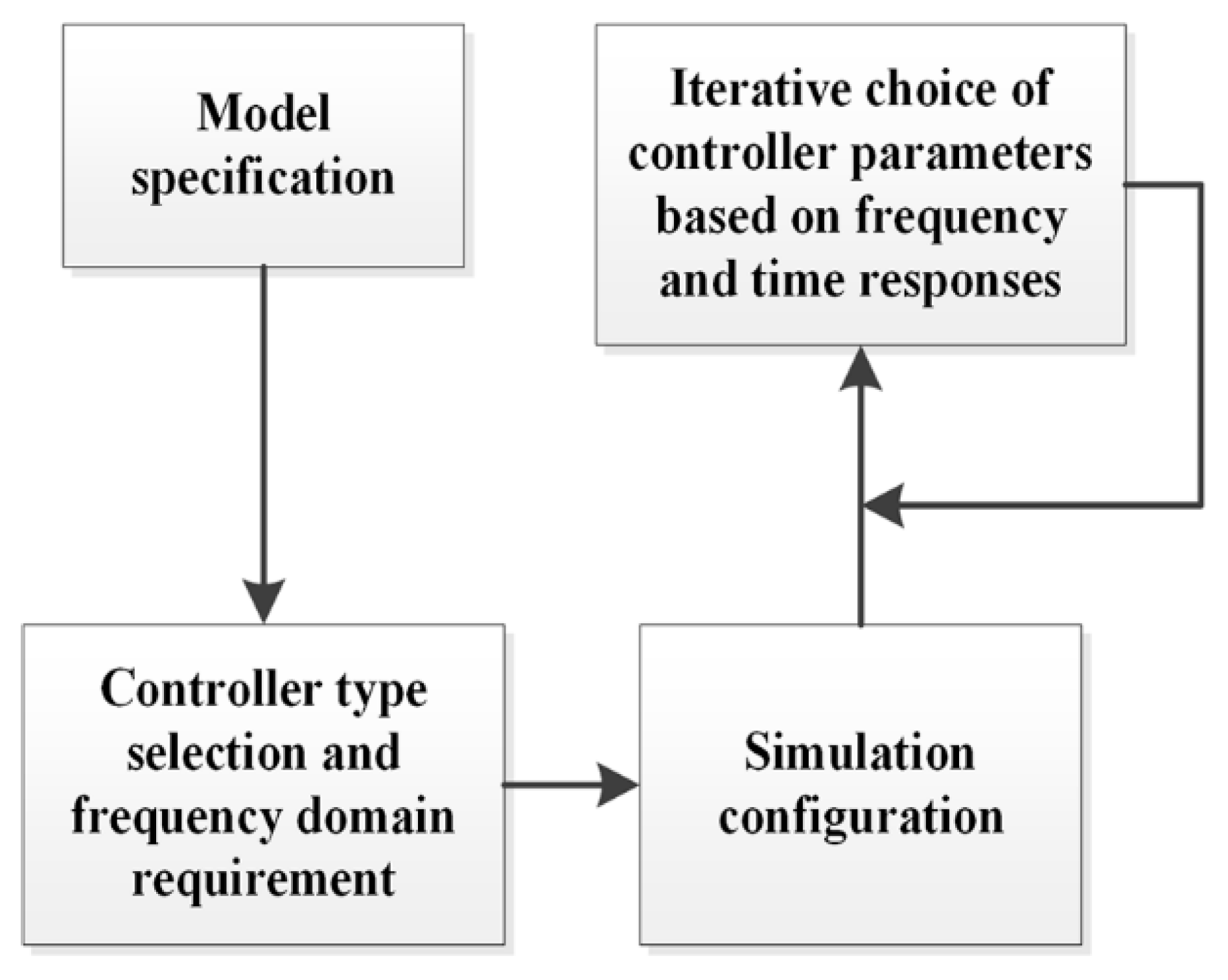
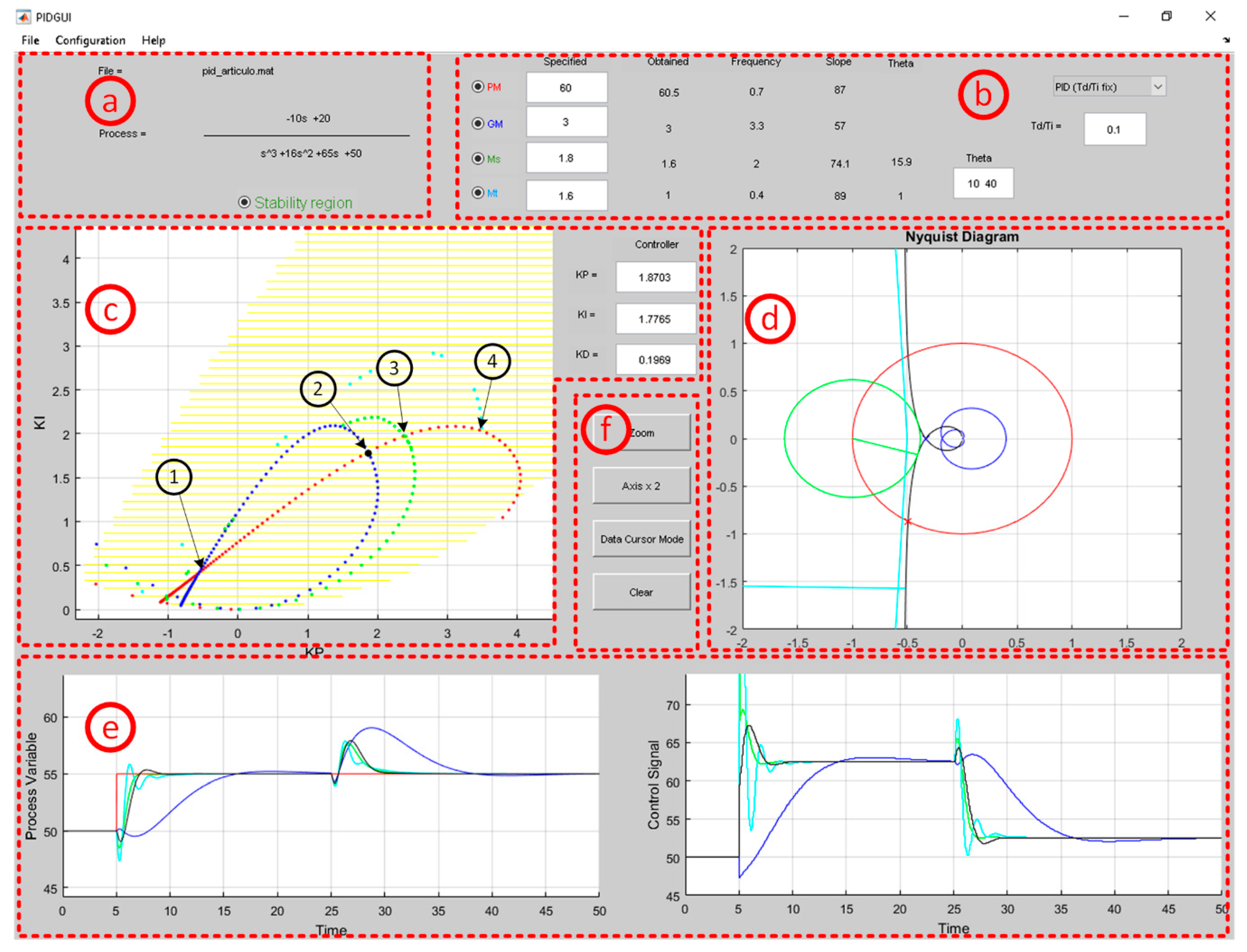
This section describes the main features of the developed interactive tool. Figure 6 describes the work flow with the tool detailing the different stages. The graphical user interface (GUI) is depicted in Figure 7. Its layout has been developed to show information about boundary curves, stability region, and frequency and time responses. The main window is divided into several differentiated parts (a–f). In the following, the main functionalities of the tool are described.
- Process transfer function (a). The transfer function of the process is shown in the upper left corner. Its numerator and denominator coefficients can be specified in the sub-menu Process in the Configuration menu.
- Frequency domain specifications and PID type (b). The kind of controller (PI, PD, PIDα, PIDKD, and PIDKI) is chosen by means of a pop-up menu located in the upper right corner. The design specifications in the frequency domain can be selected by means of radio-buttons located in the upper zone of Figure 7: Phase margin (PM), gain margin (GM), maximum sensitivity (Ms), and maximum complementary sensitivity (Mt). These requirements are specified by single values, or a range of two values, in the corresponding four text fields of the Specified column. On the right side, the truly obtained specification values for the current controller parameters are shown together with the corresponding frequencies. There is also a text field to edit the desired range of the angle θ for Ms and Mt specifications. The slope of the loop Nyquist plot in each of these frequencies, and the obtained angles θ for Ms and Mt, are also shown.
- Controller parameter space (c). This plot shows the KP-KI parameter space for the PI, PIDα, and PIDKD controllers, or the KP-KD parameter space for the PD and PIDKI controllers, according to Table 1. The boundary curves fulfilling the specified frequency requirements are plotted in different colors: Red (PM), blue (GM), green (Ms), and cyan (Mt). These curves can be displayed or hidden using the requirement radio-buttons. The values of the current control parameters (KP, KI, and KD) are visible in the three text fields placed on the right of this plot, and they are also depicted by a black point in the parameter space. The user can change the PID parameters either by dragging the aforementioned black point or by editing the corresponding text fields. Every time the controller changes, the frequency response features, Nyquist plot, and time response are updated. In addition, when the Stability region radio-button is enabled, the plot shows the set of controller parameters that stabilize the specified feedback system, delimiting this region by a set of yellow lines. If the model process is changed, this stability region is automatically updated.
- Nyquist plot (d). In this figure, the Nyquist diagram of the process P(s) is shown in blue, and the Nyquist curve of the compensated open loop L(s) is depicted in black. The unit circle and the circles for Ms and Mt are also depicted in red, green, and cyan, respectively. This information is very important to determine if the Nyquist plot shape is adequate [11]. It is updated when the controller parameters are modified.
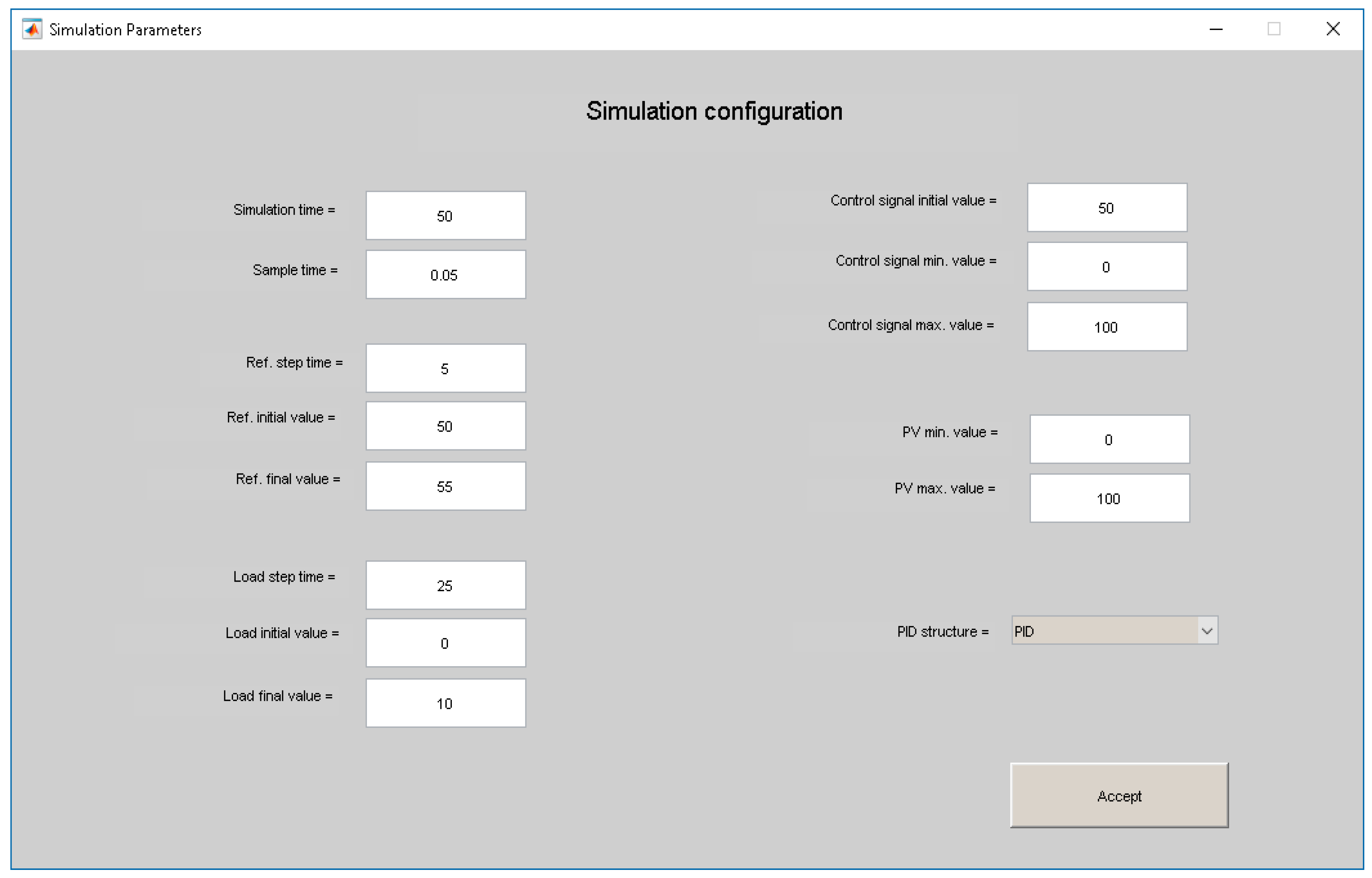
- Time response simulation (e). These plots show the temporal response of the controlled variable and control signal of the specified feedback system. Several temporal responses can be displayed. This is useful to compare different designs. This procedure can be carried out by dragging and releasing the black point of the controller parameter space to other points, or by editing the corresponding text fields. A step change in the reference signal as well as in the load disturbance can be specified for the simulation, as shown in the simulation configuration window (Figure 8), where the initial and final values are defined for both the reference and the load disturbance. This window is accessible from the sub-menu Simulation of the Configuration menu, and it also provides other text fields to specify the minimum and maximum control signal values, and process variable values, initial control signal value, simulation time, and the controller sample time. In addition, the PID structure (PID, PI-D, or I-PD) can be selected using a pop-up menu.
- Figure controls (f). This section covers a set of four buttons related with the figures. There are two toggle-buttons to enable or disable the zoom mode and the data cursor mode in all figures. The Axis x 2 button increases the axis scaling of the controller parameter space. The Clear button removes the time response simulations.
Furthermore, the toolbar of the main window incorporates additional options, where the user can save and load sessions, select several design aspects, and configure simulation parameters.
The design of the presented tool has been performed following the guidelines of similar tools, such as PIDLab (www.pidlab.com), the PID interactive learning modules based on Sysquake [20], or the PID Tuner application from Matlab. The common features are the following:
- Possibility to configure the simulation parameters.
- Possibility of modifying the model parameters of the plant and controller.
- Frequency response (Nyquist diagram) of the system.
- Closed-loop temporal response of the controlled variable and the control signal.
- Interactive zooming in the figures.
As main novelties, the proposed tool can be distinguished from others by the following features:
- Stability region in the parameter space of the KP-KI or KP-KD controller. This feature allows the selection of the controller parameters interactively. Along with it, curves of robustness specifications can also be shown, facilitating the previous task. In addition, this region is useful to compare PID designs.
- The tool allows you to analyze practical aspects, such as the choice of the sampling period and saturations of the control signals.
Educational or Training Uses
The tool provides different educational or training uses. Some of them are listed below.
- Tuning by trial and error inside the stabilizing region. The tool shows the stabilizing region in the KP-KI or KP-KD parameter space. Moving the black point in different areas of this space, the user can test the stability and closed-loop response for choosing the controller parameters.
- Comparison of PID designs. The tool offers several frequency domain specifications for PID tuning, so the user can easily compare the performance achieved with different specifications, or those obtained with the same specification at different frequencies.
- Effects of practical considerations. Practical aspects of PID controllers have been considered in the tool. Although the controller design is performed in the continuous domain, time response simulations are carried out using a discrete implementation of the controller. In addition to the effects of a bad choice of the PID controller parameters, the user can verify how a bad selection of the sampling period deteriorates the closed-loop time response. In the same way, the effects of process input saturations can be easily visualized with the tool.
4. Illustrative Example
This section shows a simple example using the tool. The purpose is controlling the non-minimum phase stable process given by the transfer function in Equation (5) using a PID controller with α of 0.1. Different frequency domain specifications and PID designs are compared, and after selecting one design, possible practical problems are analyzed. The procedure is performed in the following steps:
- Process specification: First, the coefficients of the process numerator and denominator are introduced in the Configuration/Process window in the respective textboxes.
- Controller type selection: By default, the last controller type is maintained, so PIDα type must be selected in the corresponding pop-up menu, and Td/Ti must be fixed to 0.1. Immediately, the stabilizing region in the KP-KI space for this system is calculated.
- Defining the desired frequency domain specifications: PM = 60°, GM = 3, Ms = 1.8, and Mt = 1.6. The corresponding boundary curves are depicted when they are enabled using the respective radio-buttons. Figure 7 shows the main window of this example.
- Simulation configuration: To perform the simulations, the parameters given in Figure 8 are configured. The range of the output and input process variables is from 0 to 100, and their initial values are 50. Step changes are applied from 50 to 55 in the set-point, and from 0 to 10 in the load disturbance, at times t = 5 s and t = 25 s, respectively. The total simulation time is 50 s, and the controller sample time is 0.05 s with PID structure.
- Comparing different designs: In this example, four PID designs are compared dragging the black point in the controller parameter space. All these points are above the 60° phase margin curve (red curve) and the intersections with other specifications curves. Point 1 represents the first curve intersection of PM = 60° and GM = 3 (blue curve). Point 2 is the second intersection of these boundary curves. Point 3 is located in the intersection with curve Ms = 1.8 (green curve), and point 4 with curve Mt = 1.6 (cyan curve). The corresponding PID parameters are collected in Table 5. These can also be identified in the KP-KI space in Figure 7. Their closed-loop responses are depicted in the bottom corner of Figure 7 (design 1 in blue, 2 in black, 3 in green, and 4 in cyan), and the achieved frequency performance indices and their associated frequencies are gathered in Table 5. Designs 2 and 3 obtain similar responses. Design 3 does not show overshoot; however, it has a higher inverse response and a more aggressive control signal. Design 4 achieves a greater oscillatory response and worse robustness, with the lowest gain margin and higher Ms. Design 1 shows the slowest response for tracking and disturbance rejection. Although designs 1 and 2 have practically the same frequency specifications, design 1 achieves them at very low frequencies, and consequently it has a slower response. Additionally, design 2 has a higher KI than that corresponding to design 1, which is advantageous for faster disturbance rejection. It also shows a good control signal response.
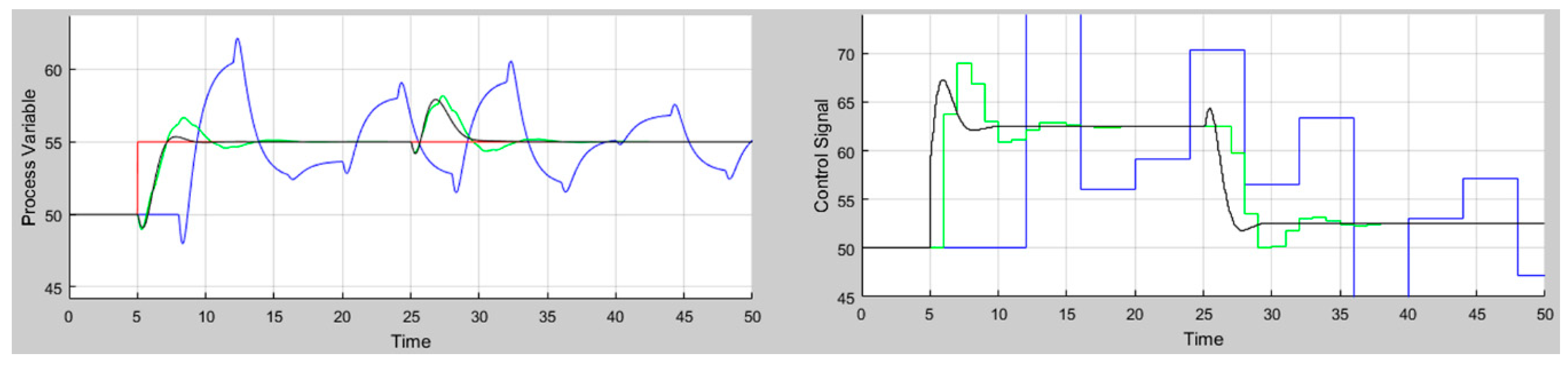
- Considering practical aspects: Assuming that design 2 is the preferred one, Figure 9 shows the closed loop time responses obtained with different controller sample times: 0.05 s (black line), 1 s (green line), and 4 s (blue line). For a sample time of 1 s, the closed-loop response is acceptable and a bit more oscillatory than that obtained with a sample time of 0.05 s. Nevertheless, the response is considerably deteriorated with a sample time of 4 s.
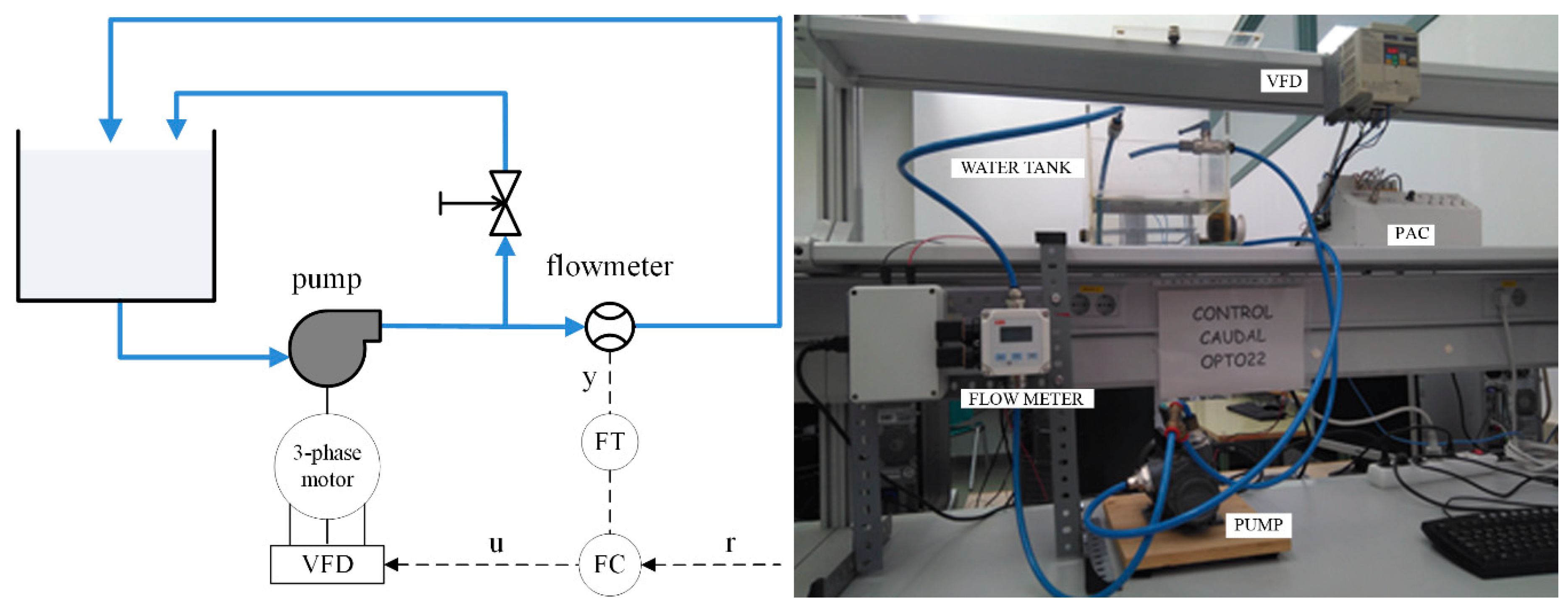
Practical Laboratory Process
In this section, the proposed tool is used for tuning a PI controller in one of our laboratory processes. Simulation results are compared to those obtained on the real system. As shown in Figure 10, the experimental process consisted of a control flow where water was pumped and returned to a tank. It was composed of a water tank, a three-phase pump taking the water from the bottom of the tank, an electromagnetic flow sensor measuring the flow rate to be controlled, and other connection elements such as valves and tubes. Part of the flow taken by the pump was returned to the tank by a manual valve, and the other part went through the branch where the flow meter was placed (see Figure 10). In this way, the maximum flow rate circulating by this second branch could be adjusted. The process also comprised a variable frequency drive (VFD) to manipulate the water flow rate. Finally, the control strategy was implemented using a programmable automation controller (PAC). The flow sensor and the VFD were connected to the PAC. The PAC was also connected to a computer for system monitoring and specifying the control parameters. The flow rate was the controlled process variable, and the manipulated variable was the operation frequency of the pump. The sampling period of the control system was 0.5 s.
First, Equation (11) shows the second order model (with a fitness of 92%) was identified for an operational point of 25 Hz:
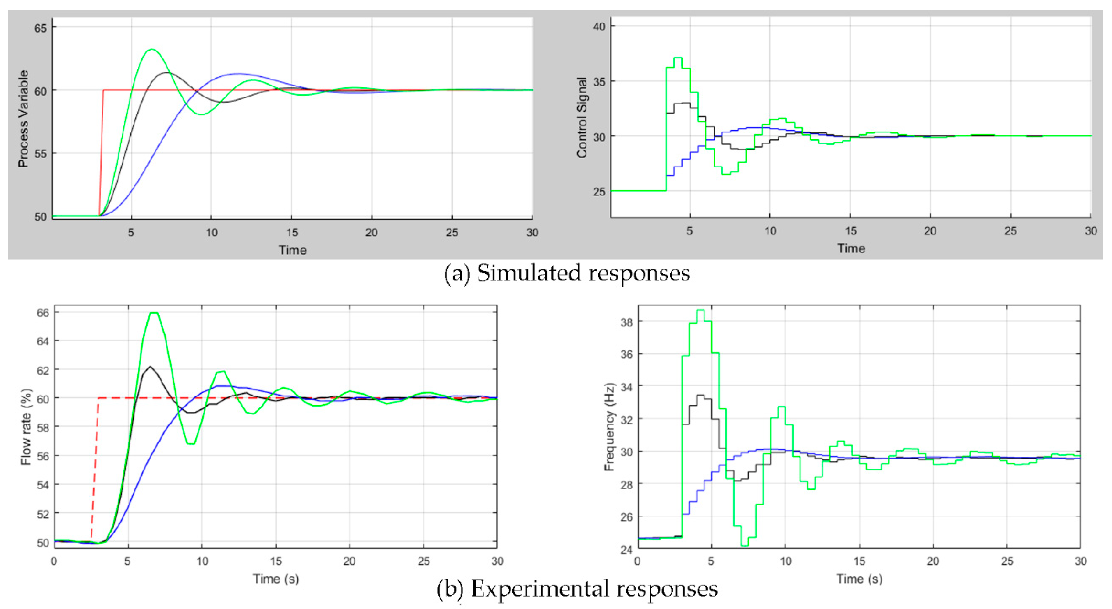
The previous model was introduced in the developed tool, and the KP and KI parameters of three different PI controllers were calculated. The control parameters and the achieved specifications are collected in Table 6. The simulated and experimental closed loop responses for each design are shown in Figure 11, where the process variable (flow rate in %) and the control signal (frequency in Hz) are depicted. A reference step of 10% was applied at t = 3 s. Although the peaks of the experimental responses were a bit higher than those obtained in simulation, there is a great similarity between the simulated (a) and the experimental (b) data. The PI 1 and PI 2 designs were tuned for a phase margin of 45° and Ms of 1.5. However, the first one provided a slower response since the corresponding frequencies ωcp and ωs were smaller than the critical frequencies of the second design. The third PI controller (PI 3) was tuned for a phase margin of 45°, maximizing the gain KI. It achieved this requirement at a ωcp of 0.9 rad/s, and it also reached a Ms of 1.7 at a ωs of 1.1 rad/s. As a consequence of the worst robustness performance, the PI 3 showed a more aggressive and oscillatory response, with a higher overshoot and greater settling time.
5. Assessment and Evaluation
This section is devoted to support assertions that the developed tool is effective in teaching basic control concepts. Enrolled students in the Automatic Control course of the Electronics Engineering degree at the University of Cordoba were asked to carry out a voluntarily set of exercises about PID controller design using the proposed tool. Then, to evaluate students’ satisfaction with the tool, students were requested to complete an anonymous electronic questionnaire, which is described next. Finally, students’ performance was evaluated considering two groups: The students of the current course using the tool, and the students of the previous year who did not use the tool. The results are discussed in the final section.
5.1. Student Survey
According to [27], a good interactive tool should include a pedagogical guideline to demonstrate important theoretical ideas, be easy to understand and use, contemplate important real-life problems, and give a good visual sensation. The proposed tool addresses these requirements in several ways:
- Theoretical ideas: Engineering students can consolidate basic concepts in process control, such as robustness specifications in the frequency domain or the design of PID controllers for stable systems comparing the final closed-loop response for several robustness margins.
- Easy to understand and use: The GUI has been designed to be user-friendly. Nevertheless, the students are guided in using the tool by the professor, who will describe the state flow shown in Figure 8.
- Real-life problem: After achieving a satisfactory tuning of PID controller parameters, it is necessary to implement the control strategy, which it is mostly performed in a discrete way. In this sense, the tool allows simulations with a discrete implementation of the PID controller, considering practical problems such as sample time effect, or process input constraints implementing an anti-windup mechanism.
- Visual sensation: The GUI is structured coherently. The information shown in the main window was reduced as much as possible to make the navigation easier. It is developed to be interactive and responsive for the user, which is a compulsory feature in the current digitalized era.
As mentioned before, to check students’ satisfaction with the tool, an online survey was carried out. Questionnaire items were collected in three subscales: Learning value, Value added, and Design usability and easy understanding of the tool. Next, the aim of each item is explained:
- -
- Learning value covers questions to analyze students’ perceptions of how effective the developed tool is to learn about PID control concepts, robustness margins, and its applicability.
- -
- Value added is aimed at assessing the use of the tool in the sense of a theoretical lecture complement.
- -
- Design usability and easy understanding of the tool evaluates students’ perceptions of the ease and clarity to navigate through the GUI.
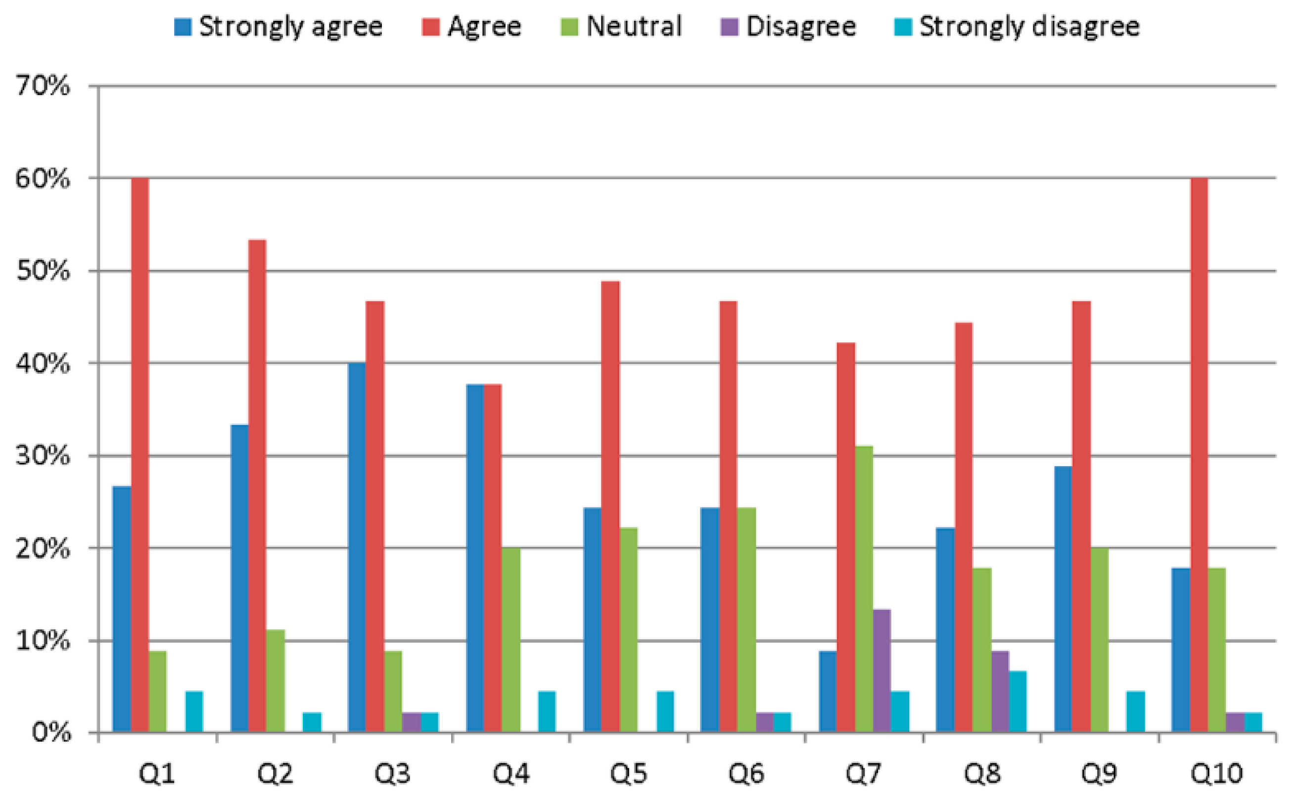
The questions were intended to collect data to study the tool contribution on the learning process of PID design in the frequency domain. The assessment and evaluation carried out was based on References [19,20,28,29,30]. The questionnaire is collected in Table 7. The first three items evaluate the Learning value. The Value-added subscale encompasses the next four items. The last three items are related to the Design usability and easy understanding of the tool. The students’ responses are summarized in Table 8. They are rated as strongly disagree, disagree, neutral, agree, or strongly agree.
Figure 12 shows the survey responses of 45 students. The percentage of strongly agree and agree answers was high compared to the rest. This points out that control engineering students emphasize the use of the proposed tool to learn and strengthen new concepts. Most students thought that concepts were clearly introduced and easy to follow, and helped them to understand the concepts of PID controllers and frequency domain specifications. However, the interactivity level did not show as good results as expected.
5.2. Student Results
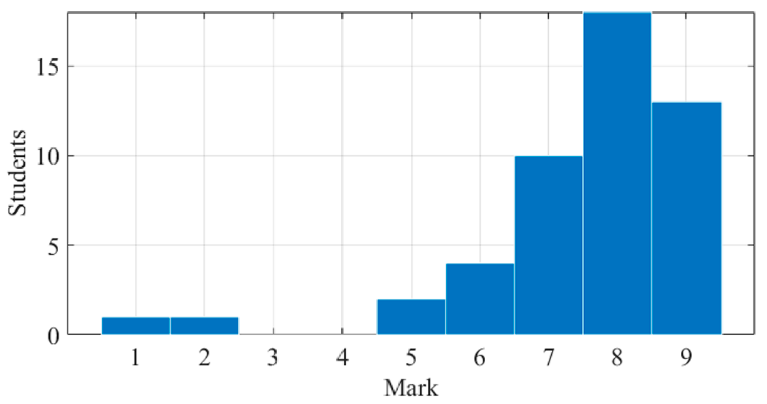
The exercises about PID controller design mentioned before were carried out voluntarily by 49 students in class. It is important to note that the students did not have a previous background related with control theory. Thus, the exercises comprised a set of basic problems and concept questions to encourage students to think about the material taught in class. The answers to the exercises were submitted through the online learning platform Moodle implemented at the University of Cordoba [31]. Figure 13 shows the mark distribution of the 49 students who submitted the proposed exercises. The average mark was 7.5.
In the current year and the previous one, students of the Automatic Control course were asked to perform a theory exam about concepts on PID control and frequency domain margins. The exam was taken by 33 students in the previous years course, and 38 students in the current one. Figure 14 shows a histogram of the scored marks for both courses—‘not using the tool’ and ‘using the tool’. The average score of students in the course using the tool was 5.8, compared to the score of 4.5 of those of the previous course who did not use it. In addition, as shown in the figure, the percentage of students who passed the exam in the current course was higher (63.9%) than the other (48.4%). A possible bias influencing the results might be that the students who utilized the tool are those who took lessons seriously. Nevertheless, the results exhibit a certain evidence that the developed tool helps students in their learning process of basic concepts of PID controllers and feedback control.
6. Conclusions
This paper has presented an interactive software tool specially focused on frequency domain tuning of PID controllers and concepts of stability, robustness, and stability margins. It contains several design methodologies according to different specifications. The developed tool is interesting for control engineering education, as well as for being used by operators in real cases. Student feedback and assessment data indicate that the learning objectives were achieved. The student response was satisfactory, showing a high degree of interest for the use of the tool as a complement to lectures, and understanding of practical problems related to controller implementation.
Author Contributions
Conceptualization, F.V. and F.M.; Methodology, J.G. and M.L.R.; Software, F.M., F.V., and J.G.; Validation and Formal Analysis, J.G. and M.L.R.; Writing—Original Draft Preparation, J.G.
Funding
This research received no external funding.
Conflicts of Interest
The authors declare no conflict of interest.
References
- Srivastava, S.; Pandit, V.S. A PI/PID controller for time delay systems with desired closed loop time response and guaranteed gain and phase margins. J. Process Control 2016, 37, 70–77. [Google Scholar] [CrossRef]
- Vilanova, R.; Alfaro, V.M. Control PID robusto: Una visión panorámica. Rev. Iberoam. Autom. Inf. Ind. RIAI 2011, 8, 141–158. [Google Scholar] [CrossRef]
- Hägglund, T.; Åström, K.J. Advanced PID Control; ISA—Instrumentation, Systems, and Automation Society: Research Triangle Park, NC, USA, 2006; ISBN 1556179421. [Google Scholar]
- Bialkowski, W.L. Control Handbook; Levine, W.S., Ed.; CRC/IEEE Press: Boca Raton, FL, USA, 1996. [Google Scholar]
- Alcántara, S.; Vilanova, R.; Pedret, C. PID control in terms of robustness/performance and servo/regulator trade-offs: A unifying approach to balanced autotuning. J. Process Control 2013, 23, 527–542. [Google Scholar] [CrossRef]
- Van Overschee, P.; Moons, C.; Van Brempt, W.; Vanvuchelen, P.; De Moor, B. RaPID: The end of heuristic PID tuning. In Proceedings of the PID ’00: IFAC Workshop on Digital Control, Terrasa, Spain, 4–7 April 2000; pp. 687–692. [Google Scholar]
- O’dwyer, A. Handbook of PI and PID Controller Tuning Rules, 2nd ed.; Imperial College Press: London, UK, 2006; Volume 26, ISBN 978-1-84816-242-6. [Google Scholar]
- Leva, A.; Maggion, M. Model-Based PI(D) Autotuning. In PID Control in the Third Millenium; Springer: London, UK, 2012; pp. 45–73. [Google Scholar]
- Ziegler, J.G.; Nichols, N.B. Optimum settings for automatic controllers. Trans. ASME 1942, 64, 759–768. [Google Scholar] [CrossRef]
- Awouda, A.E.A.; Bin Mamat, R. Refine PID tuning rule using ITAE criteria. In Proceedings of the 2010 The 2nd International Conference on Computer and Automation Engineering (ICCAE), Singapore, 26–28 February 2010; Volume 5, pp. 171–176. [Google Scholar]
- Åström, K.J.; Hägglund, T. Revisiting the Ziegler–Nichols step response method for PID control. J. Process Control 2004, 14, 635–650. [Google Scholar] [CrossRef]
- Tavakoli, S.; Safaei, M. Analytical PID control design in time domain with performance-robustness trade-off. Electron. Lett. 2018, 54, 815–817. [Google Scholar] [CrossRef]
- Arrieta, O.; Vilanova, R. Simple PID tuning rules with guaranteed Ms robustness achievement. IFAC Proc. Vol. 2011, 44, 12042–12047. [Google Scholar] [CrossRef]
- Alfaro, V.M.; Vilanova, R. Optimal robust tuning for 1DoF PI/PID control unifying FOPDT/SOPDT models. IFAC Proc. Vol. 2012, 2, 572–577. [Google Scholar] [CrossRef]
- Morilla, F.S.D. Methodologies for the Tuning of PID Controllers in the Frequency Domain. IFAC Proc. Vol. 2000, 147–152. [Google Scholar] [CrossRef]
- Morilla, F.; Vázquez, F.; Hernández, R. PID control design with guaranteed stability. IFAC Proc. Vol. 2006, 7, 13–18. [Google Scholar] [CrossRef]
- Mathworks Home Page. Available online: http://www.mathworks.com (accessed on 2 August 2018).
- Ruiz, Á.; Jiménez, J.E.; Sánchez, J.; Dormido, S. Design of event-based PI-P controllers using interactive tools. Control Eng. Pract. 2014, 32, 183–202. [Google Scholar] [CrossRef]
- Morales, D.C.; Jiménez-Hornero, J.E.; Vázquez, F.; Morilla, F. Educational tool for optimal controller tuning using evolutionary strategies. IEEE Trans. Educ. 2012, 55, 48–57. [Google Scholar] [CrossRef]
- Guzmán, J.L.; Aström, K.J.; Dormido, S.; Hägglund, T.; Berenguel, M.; Piguet, Y. Interactive learning modules for PID control. IEEE Control Syst. Mag. 2008, 28, 118–134. [Google Scholar] [CrossRef]
- Guzmán, J.L.; Dormido, S.; Berenguel, M. Interactivity in education: An experience in the automatic control field. Comput. Appl. Eng. Educ. 2013, 21, 360–371. [Google Scholar] [CrossRef]
- Aliane, N. A matlab/simulink-based interactive module for servo systems learning. IEEE Trans. Educ. 2010, 53, 265–271. [Google Scholar] [CrossRef]
- Schlegel, M.; Mertl, J. Stability regions for PI/PID controller and Matlab program. In Proceedings of the 5th International Carpathian Control Conference, Zakopane, Poland, 25–28 May 2004; AGH-UST: Krakow, Poland, 2004; pp. 1–6. [Google Scholar]
- Barmish, B.R. New tools for robustness analysis. In Proceedings of the 27th IEEE Conference on Decision and Control, Austin, TX, USA, 7–9 December 1988; pp. 1–6. [Google Scholar] [CrossRef] [Green Version]
- Ackermann, J. Parameter space design of robust control systems. IEEE Trans. Autom. Contr. 1980, 25, 1058–1072. [Google Scholar] [CrossRef]
- Dormido, S.; Morilla, F. Tuning of PID controllers based on sensitivity margin specification. In Proceedings of the 2004 5th Asian Control Conference (IEEE Cat. No.04EX904), Melbourne, Victoria, Australia, 20–23 July 2004; Volume 1, pp. 486–491. [Google Scholar]
- Balchen, J.G.; Handlykken, M.; Tysso, A. The need for better laboratory experiments in control engineering education. IFAC Proc. Vol. 1981, 14, 3363–3368. [Google Scholar] [CrossRef]
- Ruz, M.L.; Garrido, J.; Vázquez, F. Educational tool for the learning of thermal comfort control based on PMV-PPD indices. Comput. Appl. Eng. Educ. 2018. [Google Scholar] [CrossRef]
- Fragoso, S.; Ruz, M.L.; Garrido, J.; Vázquez, F.; Morilla, F. Educational software tool for decoupling control in wind turbines applied to a lab-scale system. Comput. Appl. Eng. Educ. 2016, 24, 400–411. [Google Scholar] [CrossRef]
- Sánchez, J.; Dormido, S.; Pastor, R.; Morilla, F. A Java/Matlab-Based Environment for Remote Control System Laboratories: Illustrated with an Inverted Pendulum. IEEE Trans. Educ. 2004, 47, 321–329. [Google Scholar] [CrossRef]
- Moodle Home Page. Available online: https://moodle.org/ (accessed on 2 August 2018).
Figure 1.
Feedback control system.

Figure 2.
Example of Nyquist plot of the loop transfer function and its features.

Figure 3.
Stabilizing region and ϕm = 60° boundary curve in the KP-KI parameter plane for the proportional-integral-derivative (PID)α control of the non-minimum phase process in Equation (5).
Figure 3.
Stabilizing region and ϕm = 60° boundary curve in the KP-KI parameter plane for the proportional-integral-derivative (PID)α control of the non-minimum phase process in Equation (5).

Figure 4.
Stabilizing region and different boundary curves in the KP-KI parameter plane for PIDα control of the non-minimum phase process in Equation (5).
Figure 4.
Stabilizing region and different boundary curves in the KP-KI parameter plane for PIDα control of the non-minimum phase process in Equation (5).

Figure 5.
Stabilizing region and boundary curves (Ms = 1.8 and Mt = 1.6) in the KP-KI parameter plane for PIDα control of the non-minimum phase process in Equation (5).
Figure 5.
Stabilizing region and boundary curves (Ms = 1.8 and Mt = 1.6) in the KP-KI parameter plane for PIDα control of the non-minimum phase process in Equation (5).

Figure 6.
Work flow description of the tool.

Figure 7.
Main window.

Figure 8.
Simulation configuration window.

Figure 9.
Responses with different controller sample times.

Figure 10.
Schematic of the plant and experimental setup.

Figure 11.
Simulated (a) and experimental (b) closed loop responses (PI 1 in blue color, PI 2 in black, and PI 3 in green).
Figure 11.
Simulated (a) and experimental (b) closed loop responses (PI 1 in blue color, PI 2 in black, and PI 3 in green).

Figure 12.
Students’ survey answers.

Figure 13.
Students’ marks in the proposed exercises about PID controllers.

Figure 14.
Comparison of exam scores between groups ‘using the tool’ and ‘not using the tool’.


Table 1.
Stability regions on the controller parameter plane.
| Control | Plane | Characteristic Equation |
|---|---|---|
| PI | KP-KI | fPI(s; KP, KI) = s A(s) + s KP B(s) + KI B(s) = 0 |
| PD | KP-KD | fPD(s; KP, KD) = A(s) + s KD B(s) + KP B(s) = 0 |
| PIDα | KP-KI | fα(s; KP, KI) = s KI A(s) + s2KP2α B(s) + s KP KI B(s) + KI2B(s) = 0 |
| PIDKD | KP-KI | fKD(s; KP, KI) = s AD(s) + s KP BD(s) + KI BD(s) = 0 |
| PIDKI | KP-KD | fKI(s; KP, KD) = AI(s) + s KD BI(s) + KP BI(s) = 0 |
Table 2.
Target points for the four frequency domain specifications.
| Specification | Target Point |
|---|---|
| PM (ϕm) | ϕB = ϕm; rB = 1 |
| GM (Am) | ϕB = 0°; rB = 1/Am |
| Ms (Ms, θ) c = −1 R = 1/MS | |
| Mt (Mt, θ) |
Table 3.
Boundary curves for proportional-integral-derivative (PID) control.
| Control | Boundary Curve |
|---|---|
| PIDα | |
| PIDKD | |
| PIDKI |
Table 4.
Discrete PID controller.
| Discrete PID Controller |
|---|
Table 5.
PID designs and achieved specifications.
| Design | KP | KI | KD | PM (ωcp) | GM (ωcg) | Ms (ωs) | Mt (ωt) |
|---|---|---|---|---|---|---|---|
| 1 | –0.55 | 0.4 | 0.074 | 60 (0.2) | 3 (0.5) | 1.6 (0.4) | 1 (0.1) |
| 2 | 1.87 | 1.78 | 0.196 | 60.5 (0.7) | 3 (3.3) | 1.6 (2) | 1 (0.4) |
| 3 | 2.37 | 1.96 | 0.29 | 60 (0.9) | 2.5 (3.7) | 1.8 (2.6) | 1 (1.3) |
| 4 | 3.48 | 2.03 | 0.6 | 60 (1.3) | 1.7 (4.8) | 2.5 (4) | 1.6 (3.6) |
Table 6.
Control parameters and specifications obtained from the lab test.
| Design | KP | KI | PM (ωcp) | Ms (ωs) |
|---|---|---|---|---|
| PI 1 | 0.103 | 0.155 | 60 (0.3) | 1.5 (0.5) |
| PI 2 | 0.62 | 0.26 | 60 (0.6) | 1.5 (1) |
| PI 3 | 1 | 0.42 | 45 (0.9) | 1.7 (1.1) |
Table 7.
Student questionnaire for tool assessment.
| Learning Value | |
| Q1 | Did the tool help you to visualize new concepts related to PID control design in the frequency domain? |
| Q2 | Do you think you will remember the concepts taught with the tool better than if you had only lecture classes? |
| Q3 | Do you think that the tool motivates learning and is useful as a complement to lecture explanations? |
| Value added | |
| Q4 | Were you satisfied with the simulations performed with the tool? |
| Q5 | Did the tool help you to improve your theoretical knowledge of PID tuning and robustness specifications in the frequency domain? |
| Q6 | Were you able to understand practical problems and implementation issues such as sample time choice or control signal limitations? |
| Q7 | Was the level of interactivity in the tool adequate? |
| Design usability and easy understanding of the tool | |
| Q8 | Do you think that the graphical user interface is user-friendly? |
| Q9 | Was the tool easy to understand and use? |
| Q10 | Were concepts with the tool clearly presented and easy to follow? |
Table 8.
Students’ responses to the tool survey (number of students = 45).
| Group Items | Strongly Agree | Agree | Neutral | Disagree | Strongly Disagree |
|---|---|---|---|---|---|
| Learning value (Q1, Q2, Q3) | 33% | 53% | 10% | 1% | 3% |
| Value added (Q4, Q5, Q6, Q7) | 24% | 44% | 24% | 4% | 4% |
| Design usability and easy understanding of the tool (Q8, Q9, Q10) | 23% | 50% | 19% | 4% | 4% |
© 2018 by the authors. Licensee MDPI, Basel, Switzerland. This article is an open access article distributed under the terms and conditions of the Creative Commons Attribution (CC BY) license (http://creativecommons.org/licenses/by/4.0/).
Share and Cite
MDPI and ACS Style
Garrido, J.; Ruz, M.L.; Morilla, F.; Vázquez, F. Interactive Tool for Frequency Domain Tuning of PID Controllers. Processes 2018, 6, 197. https://doi.org/10.3390/pr6100197
AMA Style
Garrido J, Ruz ML, Morilla F, Vázquez F. Interactive Tool for Frequency Domain Tuning of PID Controllers. Processes. 2018; 6(10):197. https://doi.org/10.3390/pr6100197
Chicago/Turabian StyleGarrido, Juan, Mario L. Ruz, Fernando Morilla, and Francisco Vázquez. 2018. "Interactive Tool for Frequency Domain Tuning of PID Controllers" Processes 6, no. 10: 197. https://doi.org/10.3390/pr6100197
Note that from the first issue of 2016, this journal uses article numbers instead of page numbers. See further details here.