Effect of Moisture Content on Lignocellulosic Power Generation: Energy, Economic and Environmental Impacts


1
Environmental Research Institute, MaREI Centre, University College Cork, Cork T23 E4PW, Ireland
2
School of Engineering, University College Cork, Cork T12 HW58, Ireland
Processes 2017, 5(4), 78; https://doi.org/10.3390/pr5040078
Submission received: 7 October 2017
/
Revised: 1 December 2017
/
Accepted: 4 December 2017
/
Published: 6 December 2017
(This article belongs to the Collection Process System Engineering for More Efficient Power and Chemicals Production)
Abstract
:The moisture content of biomass affects its processing for applications such as electricity or steam. In this study, the effects of variation in moisture content of banagrass and energycane was evaluated using techno-economic analysis and life-cycle assessments. A 25% loss of moisture was assumed as a variation that was achieved by field drying the biomass. Techno-economic analysis revealed that high moisture in the biomass was not economically feasible. Comparing banagrass with energycane, the latter was more economically feasible; thanks to the low moisture and ash content in energycane. About 32 GWh/year of electricity was produced by field drying 60,000 dry MT/year energycane. The investment for different scenarios ranged between $17 million and $22 million. Field-dried energycane was the only economically viable option that recovered the investment after 11 years of operation. This scenario was also more environmentally friendly, releasing 16-gCO2 equivalent/MJ of electricity produced.
1. Introduction
Climate models from the Intergovernmental Panel on Climate Change (IPCC) have predicted that the global surface temperature will increase between 0.3 °C and 4.8 °C in the 21st century [1]. Between 1880 and 2012, the mean surface temperature increased by 0.85 °C, which is alarming and needs to be controlled. Human interventions such as using fossil fuels for energy and transportation, emissions from agricultural practices, and industrial developments are reported to be the major contributors to climate change [1]. More than 40% of the emissions could be reduced if the demands of energy supply and transportation sectors are met through clean energy sources [1]. The quest for alternative energy sources have resulted in wind, solar, geothermal, tidal, hydroelectric and bioenergy sources. However, wind and solar have problems including storage and transmission losses.
Islands like Hawaii are deprived of resources for power generation. In Hawaii, more than 70% of electricity is produced from imported oil and 13% from coal [2]. By contrast, the mainland United States generated only 1% of its electricity from oil, which shows the dependency on fossil-fuel resources in these islands. At present, 3% of the electricity produced in Hawaii comes from biomass [3]. Lignocelluloses are plentiful organics accessible today, accounting for up to 50 billion tons in dry weight [4].
Different technology routes are available for processing biomass to energy. Lignocellulosic ethanol is one of the possible alternatives for producing clean energy, which requires a pre-treatment process [5]. This pre-treatment step increases the production cost, in addition to technical hindrances such as effective sugar release and inhibitor formation. Some attempts have been made to integrate first- and second-generation ethanol production to reduce production costs [6]. However, the economic feasibility and the need for electricity cannot be satisfied with liquid fuels. Unlike biochemical processes, thermochemical processes offer access to clean energy with fewer technical hindrances. In addition, thermochemical processes satisfy the needs of electricity production for a state like Hawaii that is devoid of resources. Thermochemical processing routes for producing energy include gasification, combustion, pyrolysis, hydrothermal carbonization, and hydrothermal liquefaction [7]. In combustion, an exothermic reaction happens between the fuel and an oxidant, which produces steam and other gases. Using these hot gases in a turbine or combined cycle results in potential applications such as heat and power [8]. The state of Hawaii owns 1.3 million acres of land, of which only 8% is used for cultivation [9,10]. Utilizing the unused land for the cultivation of energy crops helps produce green electricity. This green electricity reduces the economic burden, dependence on oil, and environmental impacts.
Thermochemical processes yield higher efficiencies when the moisture content of the biomass is lower. Failing to do so consumes energy to vaporize the moisture, thus reducing the efficiency of the process. For the same reason, dried biomass such as wood chips are usually preferred in thermochemical processes. When energy crops are used, field drying them reduces the moisture content of the biomass [11]. Previous studies have investigated the effect of varying moisture content in the biomass for alternative fuel production [12,13,14]. Striugas et al. used an indirect method to calculate the heat balance that controls the reciprocating grate using wet woody biomass [15]. The variation in the moisture content affects the overall viability of the process and needs further investigation.
No previous research has considered the variation of moisture content on trifold sustainability metrics including techno-economic and environmental impact analysis. These tri-fold sustainability metrics check the feasibility of a process from a multi-disciplinary angle, ensuring the process is environmentally friendly, technically feasible, and economically viable.
The objectives of this study include:
- analyzing the effect of varying moisture content of two lignocelluloses (banagrass and energycane) for electricity production;
- evaluating the techno-economic potential of power production in Maui (Hawaii);
- carrying out an energy analysis to understand the energy flow;
- conducting a life-cycle assessment to identify the environmental impacts of the thermochemical process.
2. Methods
2.1. Description
The processing plant is foreseen to be built on Maui, one of the islands in Hawaii that uses diesel as a primary source for electricity production. The use of diesel as an electricity source, in contrast to the mainland USA, indicates that the emissions will be different. This change in emissions will affect the global warming potential (GWP) and other environmental impacts. The processing plant was designed to process 60,000 dry MT/year of lignocelluloses. The processing capacity was calculated based on the land available on Maui Island. A pilot field trial was conducted, estimating different aspects of growing crops including crop yield, crop rotation, and nutrient requirements. The agricultural emissions data used in this study were based on the field trials [16,17]. One could argue that 60,000 dry MT/year is a small capacity in comparison with the mainland USA. However, the limitation here is the land availability, which determines the sizes of the processing plant.
In this study, four scenarios were considered that used two biomasses (banagrass and energycane). For banagrass “BG” was used as the acronym, while for energycane it was “EC”. When the biomass had high moisture content, the acronym “HM” was used. For field-dried biomass that had low moisture content, “LM” was used. For example, BGLM refers to the scenario that used banagrass with low moisture. The loss of moisture by field drying the biomass was assumed as 25% (Table 1).
2.2. Feedstock
Two different feedstocks were considered in this study, including banagrass and energycane. National Renewable Energy Laboratory (NREL) procedures were followed to find the composition of banagrass, while the composition of energycane was based on Kim and Dale [18]. The biomass yield, emissions, nutrient requirements, water, and agricultural machinery requirements etc. for both the biomasses was obtained from the field trials conducted on Maui. Table 1 shows the composition of both the biomasses in wet and dry basis. The harvest rate of the biomasses was 15 MT/year with a collection efficiency of 90%.
2.3. Model Development
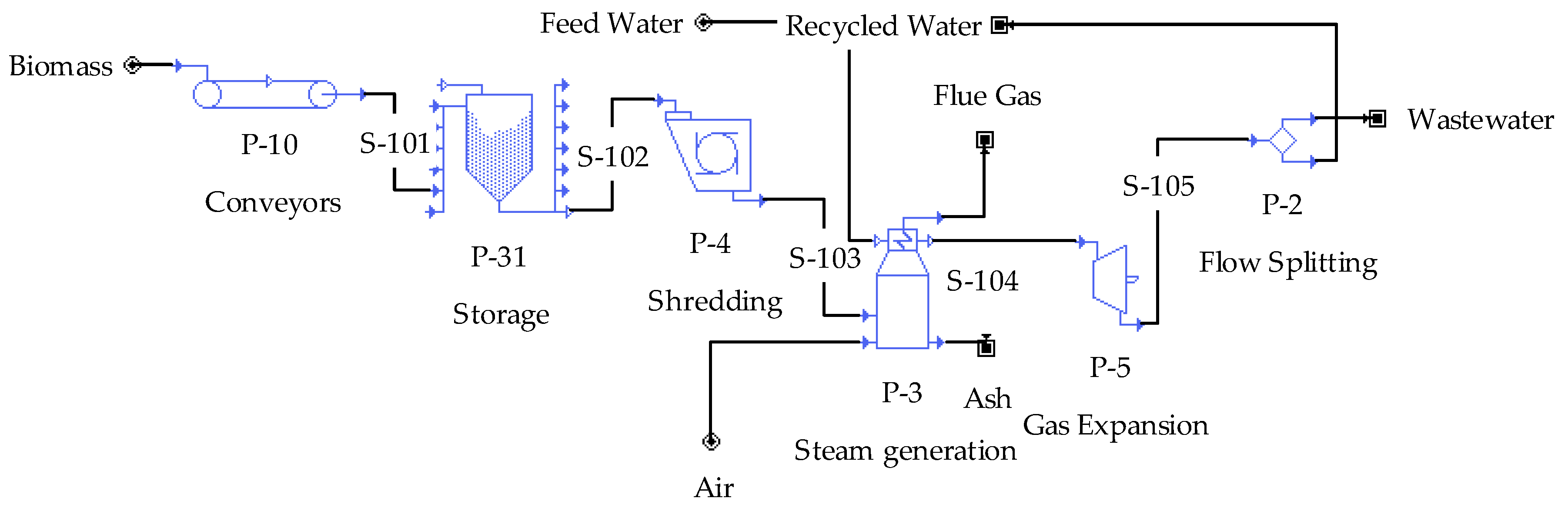
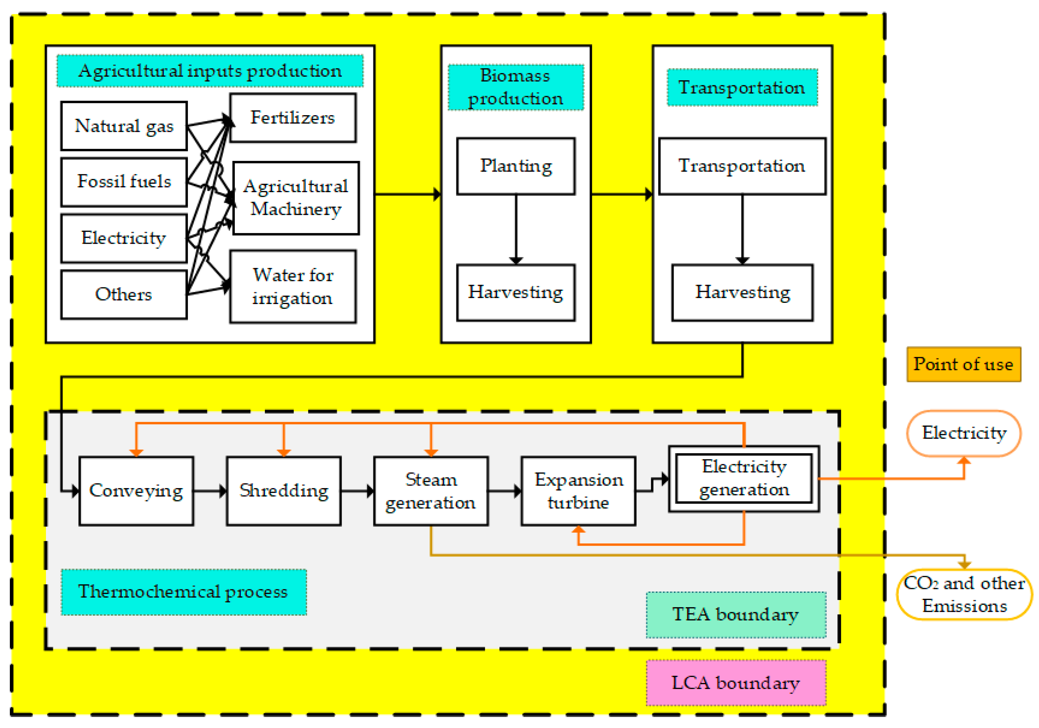
Intelligen SuperPro Designer (V-10.0) was used to simulate the process that calculates the mass and energy balance. Based on the mass and energy balance, economic analysis was performed. The biomass harvested was transported using trucks to the processing plant site. When the biomass reached the site, it was unloaded and stored in a silo using a conveyor, before it was processed. The silo had a storage capacity to hold biomass for 10 days. The stored biomass was shredded using a knife mill that used energy at the rate of 0.09 kW/(kg/h). For field-dried biomass with low moisture, 0.15 kW/(kg/h) energy was used [19]. This was due to the fact that wet biomass consumes less energy to shred, while dry biomass requires high energy. The shredded biomass was then conveyed to the boiler for steam generation. Figure 1 shows the process schematics from SuperPro Designer. The developed models were attached as Supplementary Materials to facilitate transparency and reproducibility (Supplementary Materials Files 1–4).
The boiler was operated at 257 °C and 4.5 MPa, which used 10% excess oxygen from air based on the biomass selected [20]. The excess oxygen was adjusted with the flow to provide complete combustion of the material. The flu gas exited the boiler at 200 °C, with the overall heat loss assumed to be 5% [21]. The elemental composition of individual components determined the steam production rate in the boiler. The available heat in the boiler varied, depending on the moisture content of the biomass. Ash exists in the boiler at 450 °C. The steam from the boiler was sent to a turbine, where the steam was expanded to produce electricity. The cooled steam after the gas expansion was condensed and reused in the process, and about 5% of the water was considered as losses or waste that was not recycled. The amount of feed water was auto adjusted, depending on the throughput of the biomass in each scenario. The excess electricity after utilization by the plant was sold. To avoid confusion in economic calculations, input credits were given to utilization.
2.4. Economic Analysis
2.4.1. Assumptions
It is assumed that the plant had a lifetime of 15 years with a construction period of 2.5 years and startup period of 4 months. The construction period was higher, as most of the construction materials needed to be barged from the mainland. The annual operation time of the plant was 330 days, with the remaining 35 days used for plant maintenance and other purposes. The sizing and costing of the different equipment were based on SuperPro Designer. The interest rate was assumed to be 7%, while annual inflation was presumed to be 4%. Table 2 shows the detailed assumptions that were used to carry out this study. Biomass was purchased at a cost of $80/dry MT [17]. Electricity was sold at a cost of $0.27/kWh, based on data obtained from Hawaiian Electric [22]. The straight-line depreciation method was used, and the depreciation period was assumed to be for 10 years.
2.4.2. Uncertainty Analysis
Uncertainty analysis depicts the vulnerability of a process, making it essential to understand its robustness. For this reason, different uncertainty analyses were carried, out including the fluctuation in capacity and the minimum electricity-selling price (MESP) for a zero net present value (NPV). In the base scenarios, the capacity of the plant was assumed as 60,000 dry MT/year; while for the uncertainty analysis, the capacity varied between 30,000 dry MT/year and 360,000 dry MT/year. Similarly, the selling price of electricity was altered to find the MESP, at which the process yields no profit or loss.
2.5. Life-Cycle Assessments
2.5.1. Goal, Scope and Boundary Definition
One of the goals of this work was to carry out the life-cycle assessment (LCA) using a well-to-pump life-cycle inventory and assess the environmental impacts of electricity production from two biomasses in Hawaii region. The scope included comparing environmental impacts of electricity production from lignocelluloses, to replace conventional electricity production in Hawaii, under high-moisture and low-moisture content. 1-MJ was used as a functional unit to carry out the assessment. Figure 2 shows the system boundaries, representing the techno-economic and LCA boundaries. Agricultural inputs such as machinery, irrigation water, nutrient requirement, harvesting, transportation of the biomass etc. were included in the system boundary when calculating the life-cycle assessments. Open LCA (V 1.6.3) software was used to estimate the environmental impact, while the eco-invent database (V 3.1) was used to run background connected processes integrating the inventory. TRACI 2.1 was used as an impact-assessment method, as this is the ISO-preferred method to carry out the LCA in the USA [23,24].
2.5.2. Life-Cycle Inventory
The mass and energy balance from the techno-economic analysis was used as the life-cycle inventory (LCI). The process model yielded inputs and outputs such as raw material, water consumption, energy consumption, and electricity production. The electricity from the plant was assumed to replace the electricity produced from the Hawaii electricity grid. The data for biomass production including crop yields, irrigation and field emissions were gathered based on the pilot field trials conducted in Maui, Hawaii. The eco-invent database and the imported data from the techno-economic analyses was used to conduct the LCA.
2.5.3. Life-Cycle Impact Assessments
The Tool for the Reduction and Assessment of Chemical and other Environmental Impacts (TRACI 2.1) developed by the United States Environmental Protection Agency (USEPA) was used as the life-cycle impact assessment method [25]. TRACI contains 10 different impact categories including acidification, ecotoxicity, eutrophication, global warming, ozone depletion, photochemical ozone formation (POF), resource depletion–fossil fuels, carcinogenics, non-carcinogenics, and respiratory effects [23].
3. Results
3.1. Techno-Economic Analysis
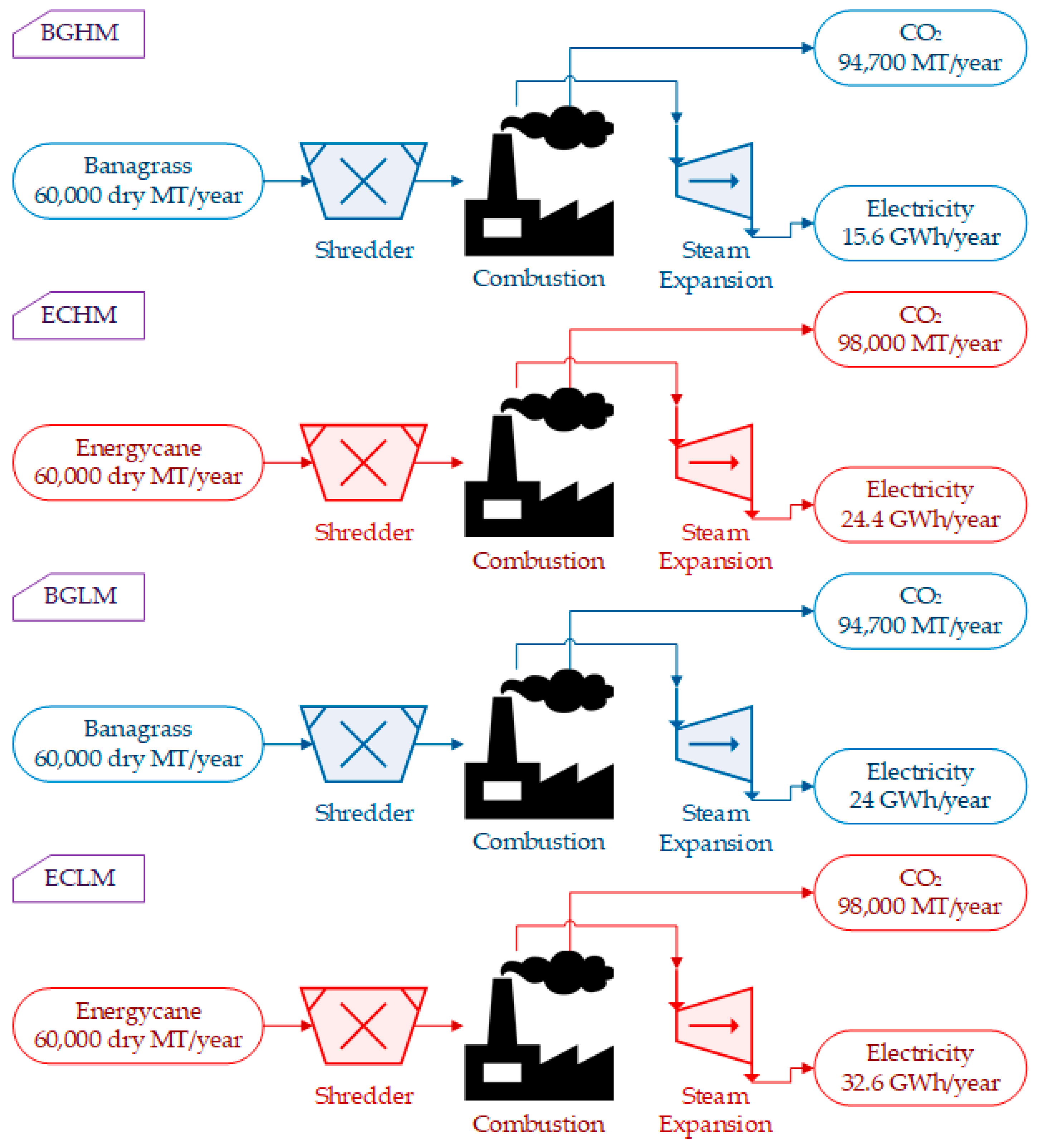
Techno-economic analysis (TEA) was carried out using SuperPro Designer (V 10.0). The change in moisture content by field drying the biomasses and their subsequent effect on the electricity production was assessed from a techno-economic perspective. The plant had an annual processing capacity of 60,000 dry MT/year in the base case. Figure 3 shows the block flow diagram of the overall mass balance of different scenarios. The moisture contents in BGHM and ECHM were 72.73% and 69.95%, respectively. The moisture content in the BGLM and ECLM scenarios was reduced to 25% in both the scenarios. Banagrass and energycane as a feedstock released 94,700 and 98,000 MT carbon dioxide/year. ECLM had the highest net electricity production (32.6 GWh/year), while, BGHM had the lowest electricity production (15.6 GWh/year) due to high moisture and low-ash content (Figure 3). The electricity reported here represents the net electricity after consumption by various elements of equipment.
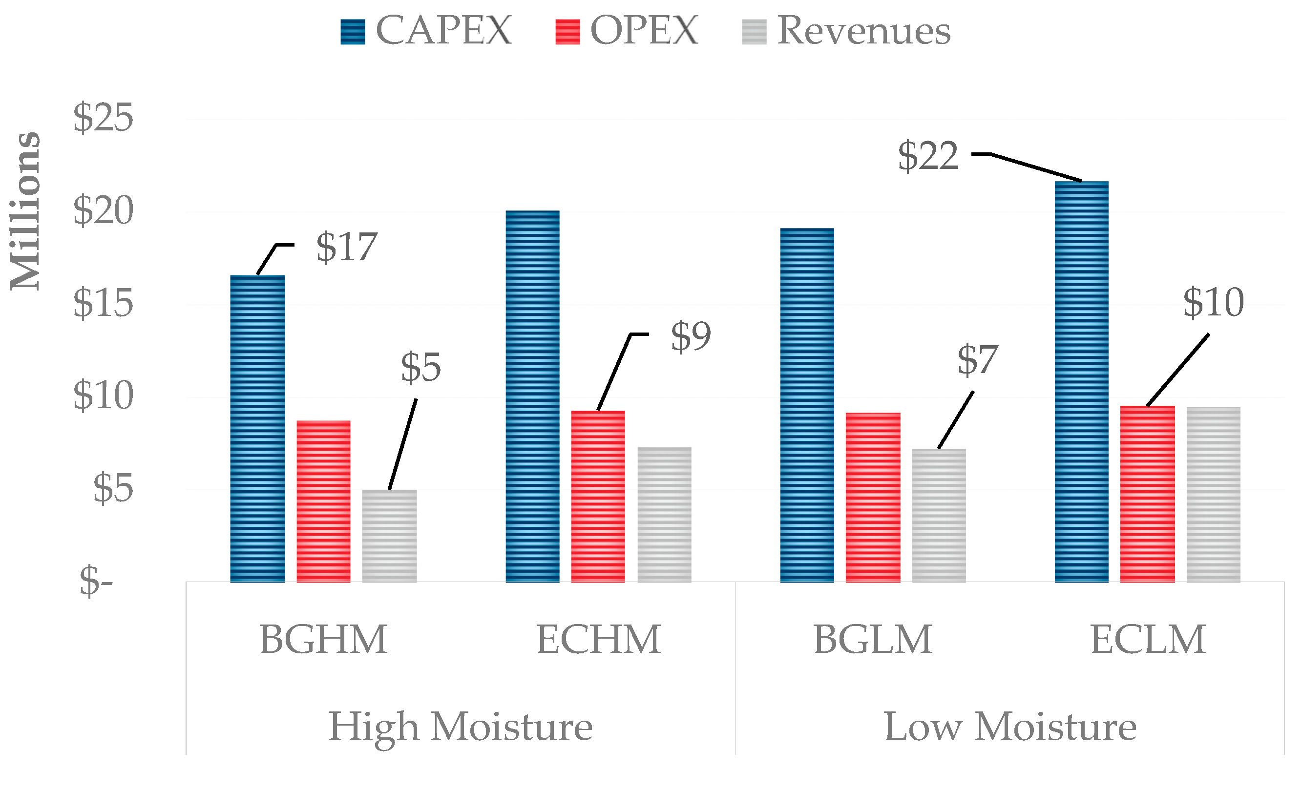
Table 3 shows the cost of different equipment used in the four scenarios with their processing throughputs. The shredder load decreased with the decrease in moisture content of the field-dried biomass. The cost of the turbines ranged between $590,000 and $1,092,000 for capacities of 2591 kW and 5922 kW. The boiler had a throughput of between 30,000 kg/h and 54,000 kg/h that cost $372,000 (BGHM) and $583,000 (ECLM). The total cost of the equipment for different scenarios ranged between $2.3 and $3.0 million. The equipment costs represents a part of the total capital investment, while the other costs include installation, piping, instrumentation, insulation, electrical, building, auxiliary facilities, indirect costs, contractor fees, and contingencies. Figure 4 shows the different economic indices including capital expenditure (CAPEX), operating expenditure (OPEX) and revenues generated from different scenarios. The capital investment ranged between $17 million and $22 million for different scenarios. In general, low-moisture content scenarios by field drying the biomass increased the CAPEX. This was due to the use of a higher capacity boiler and turbines.
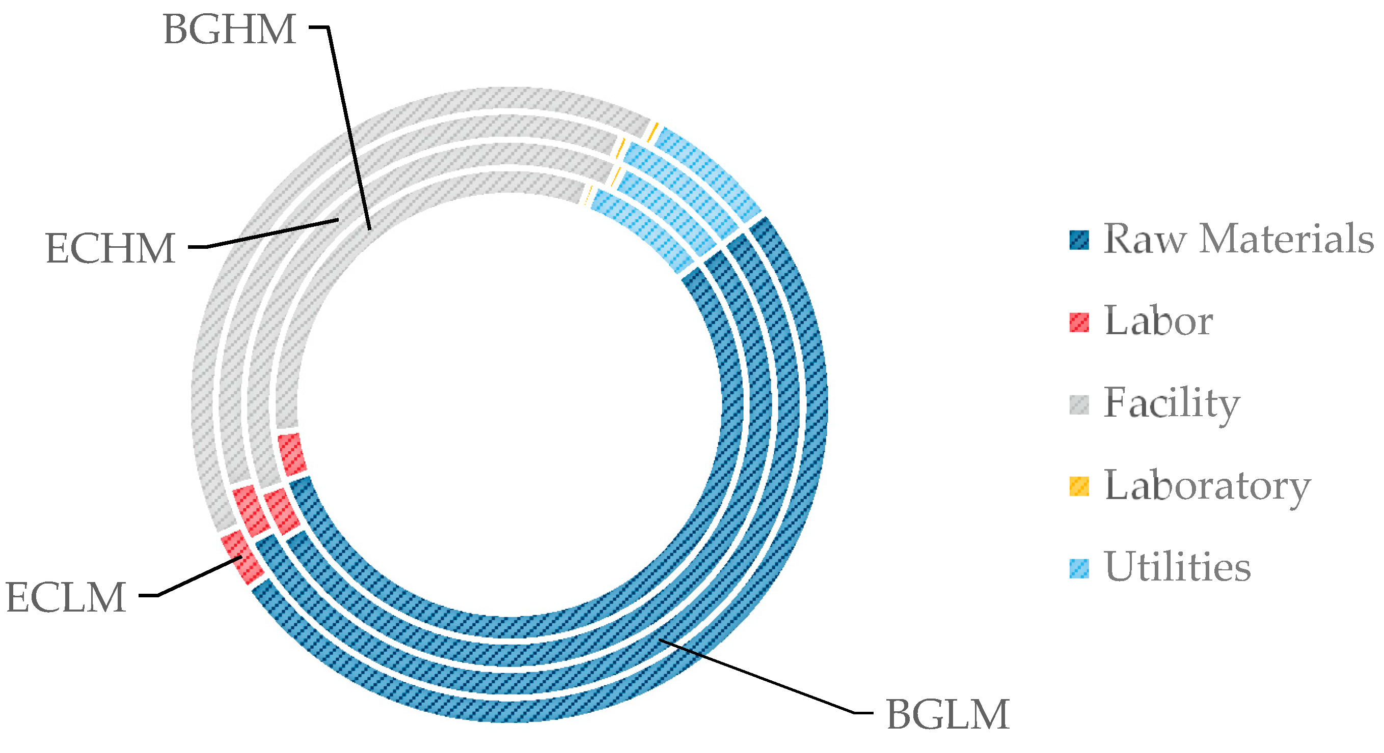
The OPEX varied between $8.7 million and $9.5 million for all the scenarios. Recovering the OPEX through revenues was only possible from the ECLM scenario (Figure 4). For all scenarios, the cost of the feedstock at $80/dry MT accounted for ca. 50% of the OPEX (Figure 5). Raw material was the most significant contributor to OPEX followed by facility-dependent costs that ranged between 32% and 39%. This shows that the cost of producing biomass needs to be controlled for any biomass-based energy/chemicals; failing to do so questions the economic viability of the project. Utilities consumption corresponds to 7–9%, while the wages for the labour was 3% of OPEX.
Every kWh of electricity sold generated a unit revenue of $0.27. The production costs for the different scenarios including BGHM, ECHM, BGLM and ECLM were $0.47, $0.34, $0.34 and $0.27, respectively (Figure 6). The production cost was recovered only in the ECLM scenario. Return on investment (ROI) corresponds to the rate at which investments yields profits. ECLM had a positive ROI at 9%, while the rest of the scenarios yielded less than 0%. Out of four scenarios considered, field-drying energycane was the only economically feasible option. However, drying the biomass results in a land-use change and those effects need to be evaluated in the future.
3.2. Energy Analysis
Figure 7 shows the energy analysis via a Sankey diagram based on the breakdown of consumption and production patterns. For scenario BGHM, about 15% of the produced electricity was consumed in different forms including a shredder, conveyors, general load and unlisted equipment. Similarly, for other scenarios, i.e., BGLM, ECHM and ECLM the consumption was 9.5%, 10.1% and 6.8%, respectively. The shredder dominated ca. 70% of the electricity consumed. The net electricity production for different scenarios was 15,653 (BGHM), 24,433 (BGLM), 24,005 (ECHM) and 32,696 (ECLM) MWh/year. It is worth mentioning that LM scenarios had higher electricity consumption for shredder (0.15 kW/(kg/h)) than HM scenarios (0.09 kW/(kg/h). However, the LM scenarios produced more electricity in comparison with HM scenarios.
3.3. Life-Cycle Assessments
The data from techno-economic assessments and field data from pilot trials were used for LCI, while LCA was conducted using Open LCA. TRACI 2.1 was used as an impact-assessment method to evaluate environmental impacts [26]. 1-MJ was used as a functional unit for all the scenarios. Seven environment-related and three health-related impacts were tabulated in Table 4 for different scenarios. For both the substrates, low-moisture scenarios resulted in lower environmental impacts in comparison with high-moisture scenarios. This shows that field drying the biomass has a positive effect on the environmental impacts; however, the effect of land-use change needs to be assessed, as the biomass will be on the field for a longer period.
Acidification refers to the increase in hydrogen ions i.e., a number of acids entering into the environment by carrying out this process. The acidification potential was measured in kg SO2 equivalent. The banagrass with high-moisture content scenario had the highest acidification potential of 3.0 × 10⁻³, while the lowest was for ECLM (9.3 × 10⁻⁴). Global warming potential was measured in kg CO2 equivalent. Every 1-MJ of electricity produced in Maui using the thermochemical process resulted in GWP between 1.6 × 10⁻¹ and 2.9 × 10⁻² kg CO2 equivalent. The same trend was observed in other environmental impacts, where BG had higher environmental impacts in comparison with EC. Similarly, HM scenarios had higher impacts in comparison with LM scenarios.
4. Discussion
4.1. Uncertainty Analysis
The base scenarios considered an annual processing capacity of 60,000 dry MT/year, which is relatively small considering the plant sizes in the mainland US. For this reason, an uncertainty analysis was carried out identifying the CAPEX of the process under different capacities. The capacities considered were between 30,000 dry MT/year and 360,000 dry MT/year. Figure 8 shows the uncertainty analysis on the CAPEX for different scenarios evaluated in the base case. As a rule of thumb by economies of scale, when the capacity increases the CAPEX goes down. To process 1-MT of biomass (BGLM) with a plant capacity of 30,000 dry MT/year, it costs $390/MT; while the same scenario operating at 360,000 dry MT/year costs $200/MT following the economies of scale principle. Increasing the capacity of the processing plant by 12 times from 30,000 dry MT/year, decreased the CAPEX by 95% on a functional unit level i.e., $/MT. It is worth mentioning that the base scenario had a processing capacity of 60,000 dry MT/year that costs $320/MT (BGLM).
4.2. Minimum Electricity Selling Price
The minimum electricity-selling price refers to the minimum costs at which the electricity needs to be sold for a zero NPV. MESP also refers to the levelized cost of electricity (LCOE) that means the cost that is incurred over the processing plant’s life to produce the total amount of energy during the same period. Figure 9 shows the MESP along with the production cost and unit revenue generated for each of the four scenarios. Under the scenarios including BGLM, ECHM, electricity needs to be sold at $0.42/kWh to meet a zero NPV while for BGHM, it should be $0.60/kWh. The most profitable scenario, ECLM, needs to sell at 6 cents higher than the current unit revenue generated to have a zero NPV i.e., $0.27/kWh. ECLM could recover the investments after 11 years (payback period). The LCOE of using different technologies including photovoltaics, wind, geothermal and nuclear that provide electricity in the Hawaiian Islands ranged between $0.1–0.5/kWh [22]. The ECLM (this study) would be on a median in comparison with the data reported; showing that further reduction in biomass costs could favor the commercialization of biomass-based power production.
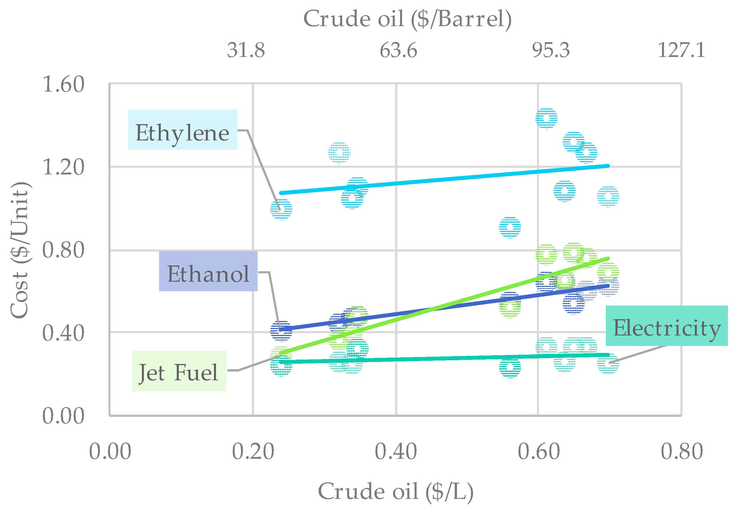
4.3. Interrelationship with Other Commodities
Relating the electricity with other commodities/energy would offer interesting insights into how the electricity would influence other energy types. For this reason, a correlation was built between the historical energy/commodity and crude oil prices from 2007 to 2016 (Figure 10). This decade-long comparison shows that the electricity prices were not fluctuating with crude oil prices, whereas other fuels including ethanol, and jet fuel were fluctuating. Ethylene was the most volatile commodity fluctuating with crude oil prices. It is worth mentioning that crude oil prices fluctuated in two regions: (1) <$63/Barrel and (2) >$95/Barrel.
4.4. Comparison with Literature
This study has reported the production cost of energy (LCOE) between $270/MWh and $470/MWh. Patel, et al. [27] compared different thermochemical technologies and reported that the production costs varied between $80/MWh and $600/MWh depending on the feedstock and technologies employed. It is worth mentioning that this study fits within this range. In addition, the study used biomass at $80/dry MT, which needs to be noted for a fair comparison with the literature. The LCA of power generation from forest biomass had GHG emissions between 7 gCO2/MJ and 15 gCO2/MJ, while this study reported between 16 gCO2/MJ and 29 gCO2/MJ [28]. The variation in GHG emissions could be based on the difference in feedstock used, which sequesters different amounts of carbon from the atmosphere.
A study reported between 2% and 4% of the produced energy [29] was consumed for internal purposes, whereas in our work the consumption of produced energy ranged between 7% and 15%. This is higher than other studies have reported, however, considering the small plant size, higher losses and greater energy utilization could be justified. This work earlier mentioned that a higher moisture content of biomass results in higher emissions, which were also confirmed by other work [30,31]. The use of a smaller plant size increased the overall emissions, as a higher plant size would be more energy efficient, thus reducing GHG emissions.
5. Conclusions
Lignocellulosic electricity production was evaluated through a holistic approach, including techno-economic analysis and life-cycle assessments, under varying moisture contents. The results suggest that drying energycane on the field was the most sustainable scenario in terms of technology, economics and environmental impacts. The most profitable scenario (ECLM) could yield investments after 11 years with a capacity of 60,000 dry MT/year. Biomass cost ($80/dry MT) was identified as the main factor affecting the profitability of the plant, followed by electricity-selling prices. The GHG emissions from different scenarios ranged between 16 gCO2/MJ and 29 gCO2/MJ. For an island like Hawaii, electricity generation from biomass could be sustainable in terms of technology, economics and environmental impact in comparison with fossil-fuel sources.
Supplementary Materials
The following are available online at https://www.mdpi.com/2227-9717/5/4/78/s1, https://doi.org/10.5281/zenodo.1069479, Files 1–4: SuperPro files can be accessed using the demo version of the software from http://www.intelligen.com/.
Acknowledgments
The author would like to thank the pilot facility in Hawaii that helped with field trial agricultural data to carry out the life-cycle assessments. Thanks go also to the Science Foundation Ireland (SFI) funded research center MaREI (Center for Marine and Renewable Energy), for providing facilities and research support.
Author Contributions
K.R. was responsible for the idea, model development, critical analysis, manuscript preparation, and editing.
Conflicts of Interest
The author declares no conflict of interests.
Acronyms
| BG | banagrass |
| CAPEX | capital costs |
| EC | energycane |
| GWP | global warming potential |
| HM | high moisture |
| LCA | life-cycle assessments |
| LCI | life-cycle inventory |
| LCOE | levelized cost of electricity |
| LM | low moisture |
| MESP | minimum electricity selling price |
| NPV | net present value |
| OPEX | operational costs |
| PBP | payback period |
| ROI | return on investment |
| TEA | techno-economic analysis |
References
- Stocker, T. Climate Change 2013: The Physical Science Basis: Working Group I Contribution to the Fifth Assessment Report of the Intergovernmental Panel on Climate Change; Cambridge University Press: Cambridge, UK, 2014. [Google Scholar]
- Department of Business Economic Development and Tourism. Monthly Energy Trends. Available online: http://dbedt.hawaii.gov/economic/data_reports/energy-trends/ (accessed on 7 October 2017).
- US Energy Information Administration. Short-Term Energy Outlook. Available online: https://www.eia.gov/outlooks/steo/report/global_oil.cfm (accessed on 7 April 2017).
- Rajendran, K.; Taherzadeh, M.J. Pretreatment of lignocellulosic materials. In Bioprocessing of Renewable Resources to Commodity Bioproducts; Bisaria, V.S., Kondo, A., Eds.; John Wiley & Sons: Hoboken, NJ, USA, 2014; pp. 43–75. [Google Scholar]
- Rajendran, K.; Drielak, E.; Varma, V.S.; Muthusamy, S.; Kumar, G. Updates on the pretreatment of lignocellulosic feedstocks for bioenergy production—A review. Biomass Convers. Biorefin. 2017. [Google Scholar] [CrossRef]
- Rajendran, K.; Rajoli, S.; Taherzadeh, M.J. Techno-economic analysis of integrating first and second-generation ethanol production using filamentous fungi: An industrial case study. Energies 2016, 9, 359. [Google Scholar] [CrossRef]
- Shen, Y.; Jarboe, L.; Brown, R.; Wen, Z. A thermochemical-biochemical hybrid processing of lignocellulosic biomass for producing fuels and chemicals. Biotechnol. Adv. 2015, 33, 1799–1813. [Google Scholar] [CrossRef] [PubMed]
- Schmidt-Rohr, K. Why combustions are always exothermic, yielding about 418 kJ per mole of O2. J. Chem. Educ. 2015, 92, 2094–2099. [Google Scholar] [CrossRef]
- Surles, T.; Foley, M.; Turn, S.; Staackmann, M. A Scenario for Accelerated Use of Renewable Resources for Transportation Fuels in Hawaii; University of Hawaii, Hawaii Natural Energy Institute, School of Ocean and Earth Science and Technology: Honolulu, HI, USA, 2009. [Google Scholar]
- Phillips, V.D.; Singh, D.; Merriam, R.A.; Khan, M.A. Land available for biomass crop production in Hawaii. Agric. Syst. 1993, 43, 1–17. [Google Scholar] [CrossRef]
- Khanchi, A.; Birrell, S. Drying models to estimate moisture change in switchgrass and corn stover based on weather conditions and swath density. Agric. For. Meteorol. 2017, 237–238, 1–8. [Google Scholar] [CrossRef]
- Fortier, J.; Truax, B.; Gagnon, D.; Lambert, F. Allometric equations for estimating compartment biomass and stem volume in mature hybrid poplars: General or site-specific? Forests 2017, 8, 309. [Google Scholar] [CrossRef]
- Manzone, M.; Gioelli, F.; Balsari, P. Kiwi clear-cut: First evaluation of recovered biomass for energy production. Energies 2017, 10, 1837. [Google Scholar] [CrossRef]
- Uson, A.A.; López-Sabirón, A.M.; Ferreira, G.; Sastresa, E.L. Uses of alternative fuels and raw materials in the cement industry as sustainable waste management options. Renew. Sustain. Energy Rev. 2013, 23, 242–260. [Google Scholar] [CrossRef]
- Striūgas, N.; Vorotinskienė, L.; Paulauskas, R.; Navakas, R.; Džiugys, A.; Narbutas, L. Estimating the fuel moisture content to control the reciprocating grate furnace firing wet woody biomass. Energy Convers. Manag. 2017, 149, 937–949. [Google Scholar] [CrossRef]
- Rajendran, K.; Murthy, G.S. How does technology pathway choice influence economic viability and environmental impacts of lignocellulosic biorefineries? Biotechnol. Biofuels 2017, 10, 268. [Google Scholar] [CrossRef] [PubMed]
- Kadhum, H.J.; Rajendran, K.; Murthy, G.S. Effect of solids loading on ethanol production: Experimental, economic and environmental analysis. Bioresour. Technol. 2017, 244, 108–116. [Google Scholar] [CrossRef] [PubMed]
- Kim, M.; Day, D.F. Composition of sugar cane, energy cane, and sweet sorghum suitable for ethanol production at louisiana sugar mills. J. Ind. Microbiol. Biotechnol. 2011, 38, 803–807. [Google Scholar] [CrossRef] [PubMed]
- Lee, J.H.; Kwon, J.H.; Kim, T.H.; Choi, W.I. Impact of planetary ball mills on corn stover characteristics and enzymatic digestibility depending on grinding ball properties. Bioresour. Technol. 2017, 241, 1094–1100. [Google Scholar] [CrossRef] [PubMed]
- Ali Mandegari, M.; Farzad, S.; Görgens, J.F. Economic and environmental assessment of cellulosic ethanol production scenarios annexed to a typical sugar mill. Bioresour. Technol. 2017, 224, 314–326. [Google Scholar] [CrossRef] [PubMed]
- Ali Mandegari, M.; Farzad, S. Görgens jf. In Biofuels: Production and Future Perspectives; Singh, R.S., Panday, A., Gnansounou, E., Eds.; CRC Press: Boca Raton, FL, USA, 2016. [Google Scholar]
- Hawaii State Energy Office. Hawaii Energy Facts & Figures; Hawaii State Energy Office: Honolulu, HI, USA, 2014; pp. 1–27.
- Bare, J.; Young, D.; Qam, S.; Hopton, M.; Chief, S. Tool for the Reduction and Assessment of Chemical and Other Environmental Impacts (TRACI); US Environmental Protection Agency: Washington, DC, USA, 2012.
- ISO Technical Committee. Environmental Management: Life Cycle Assessment: Requirements and Guidelines; International Organization for Standardization (ISO): Geneva, Switzerland, 2006. [Google Scholar]
- Bare, J.C. Traci. J. Ind. Ecol. 2002, 6, 49–78. [Google Scholar] [CrossRef]
- Bare, J. Traci 2.0: The tool for the reduction and assessment of chemical and other environmental impacts 2.0. Clean Technol. Environ. 2011, 13, 687–696. [Google Scholar] [CrossRef]
- Patel, M.; Zhang, X.; Kumar, A. Techno-economic and life cycle assessment on lignocellulosic biomass thermochemical conversion technologies: A review. Renew. Sustain. Energy Rev. 2016, 53, 1486–1499. [Google Scholar] [CrossRef]
- Thakur, A.; Canter, C.E.; Kumar, A. Life-cycle energy and emission analysis of power generation from forest biomass. Appl. Energy 2014, 128, 246–253. [Google Scholar] [CrossRef]
- Wihersaari, M. Greenhouse gas emissions from final harvest fuel chip production in Finland. Biomass Bioenergy 2005, 28, 435–443. [Google Scholar] [CrossRef]
- Whittaker, C.; Mortimer, N.; Murphy, R.; Matthews, R. Energy and greenhouse gas balance of the use of forest residues for bioenergy production in the UK. Biomass Bioenergy 2011, 35, 4581–4594. [Google Scholar] [CrossRef] [Green Version]
- Angus-Hankin, C.; Stokes, B.; Twaddle, A. The transportation of fuelwood from forest to facility. Biomass Bioenergy 1995, 9, 191–203. [Google Scholar] [CrossRef]
Figure 1.
Schematics of the flowsheet developed in SuperPro Designer.

Figure 2.
System boundary showing the techno-economic (TEA) and life-cycle assessment (LCA) boundary for the lignocellulosic power production. Grey color represents the TEA boundary, while the yellow color represents the LCA boundary.
Figure 2.
System boundary showing the techno-economic (TEA) and life-cycle assessment (LCA) boundary for the lignocellulosic power production. Grey color represents the TEA boundary, while the yellow color represents the LCA boundary.

Figure 3.
Block flow diagram showing the mass balance for different scenarios. BG and EC refer to banagrass and energycane; HM and LM refer to high moisture and low moisture respectively.
Figure 3.
Block flow diagram showing the mass balance for different scenarios. BG and EC refer to banagrass and energycane; HM and LM refer to high moisture and low moisture respectively.

Figure 4.
Economic indices including capital expenditure (CAPEX), operating expenditure (OPEX) and revenues generated from different scenarios (million USD).
Figure 4.
Economic indices including capital expenditure (CAPEX), operating expenditure (OPEX) and revenues generated from different scenarios (million USD).

Figure 5.
Fragmentation of operational costs for different scenarios.

Figure 6.
Profitability indexes including production cost ($/kWh), unit revenue ($/kWh) and return on investment (%) for the four different scenarios exploited in this study.
Figure 6.
Profitability indexes including production cost ($/kWh), unit revenue ($/kWh) and return on investment (%) for the four different scenarios exploited in this study.

Figure 7.
Energy analyses of different scenarios including consumption and production of electricity: (a) BGHM; (b) BGLM; (c) ECHM; (d) ECLM. All the numbers here are presented as MWh.
Figure 7.
Energy analyses of different scenarios including consumption and production of electricity: (a) BGHM; (b) BGLM; (c) ECHM; (d) ECLM. All the numbers here are presented as MWh.
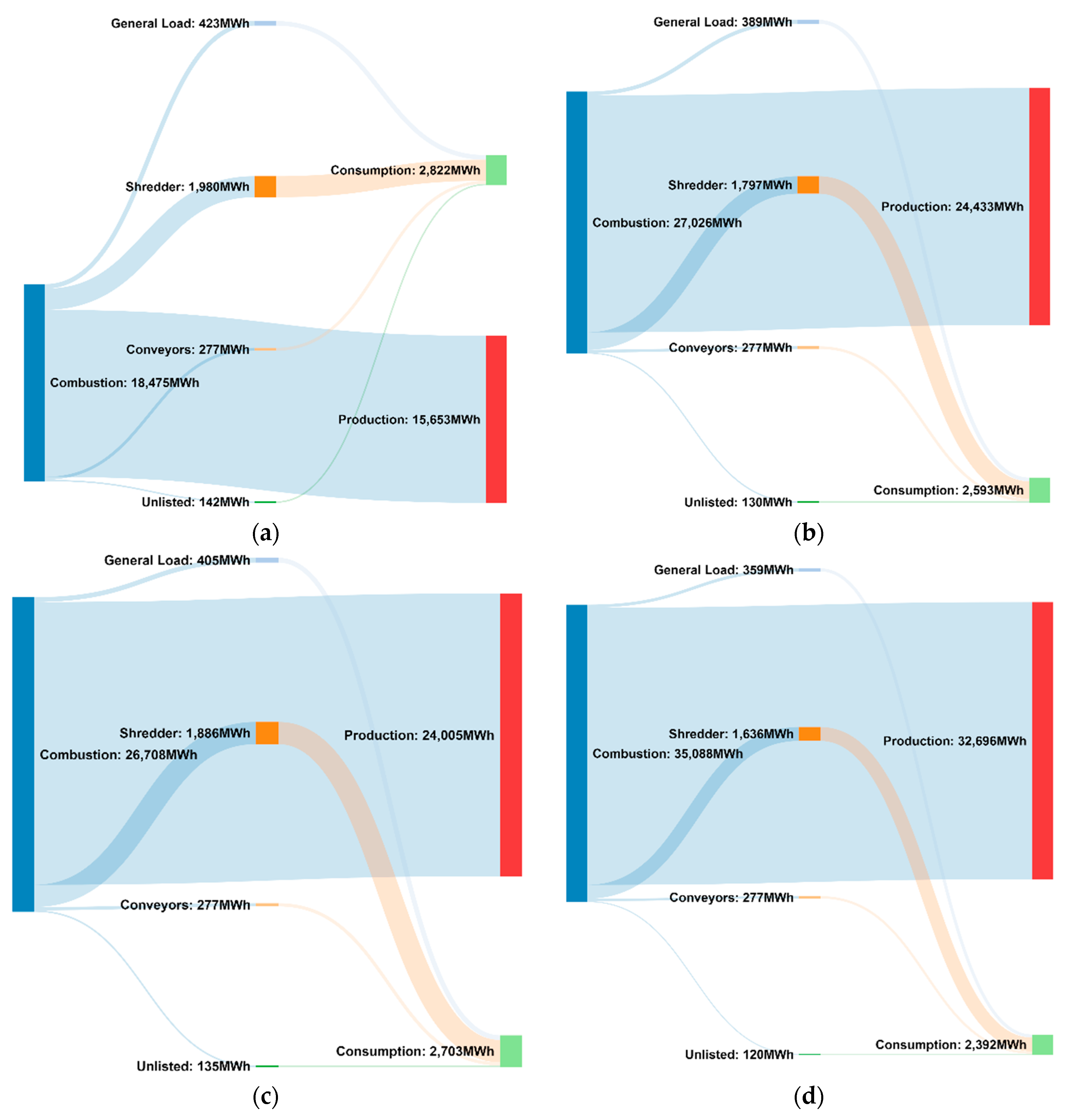
Figure 8.
Uncertainty analyses of various scenarios under different capacities between 30,000 dry MT/year and 360,000 dry MT/year.
Figure 8.
Uncertainty analyses of various scenarios under different capacities between 30,000 dry MT/year and 360,000 dry MT/year.
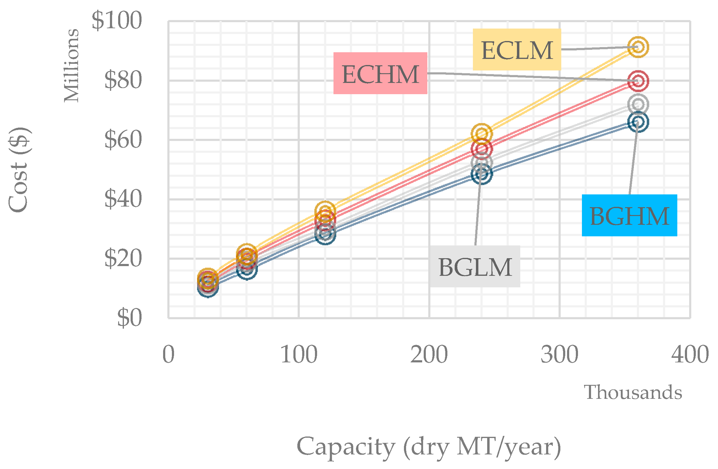
Figure 9.
Minimum electricity selling price estimation in relation to production cost and selling price for different scenarios in $/kWh.
Figure 9.
Minimum electricity selling price estimation in relation to production cost and selling price for different scenarios in $/kWh.
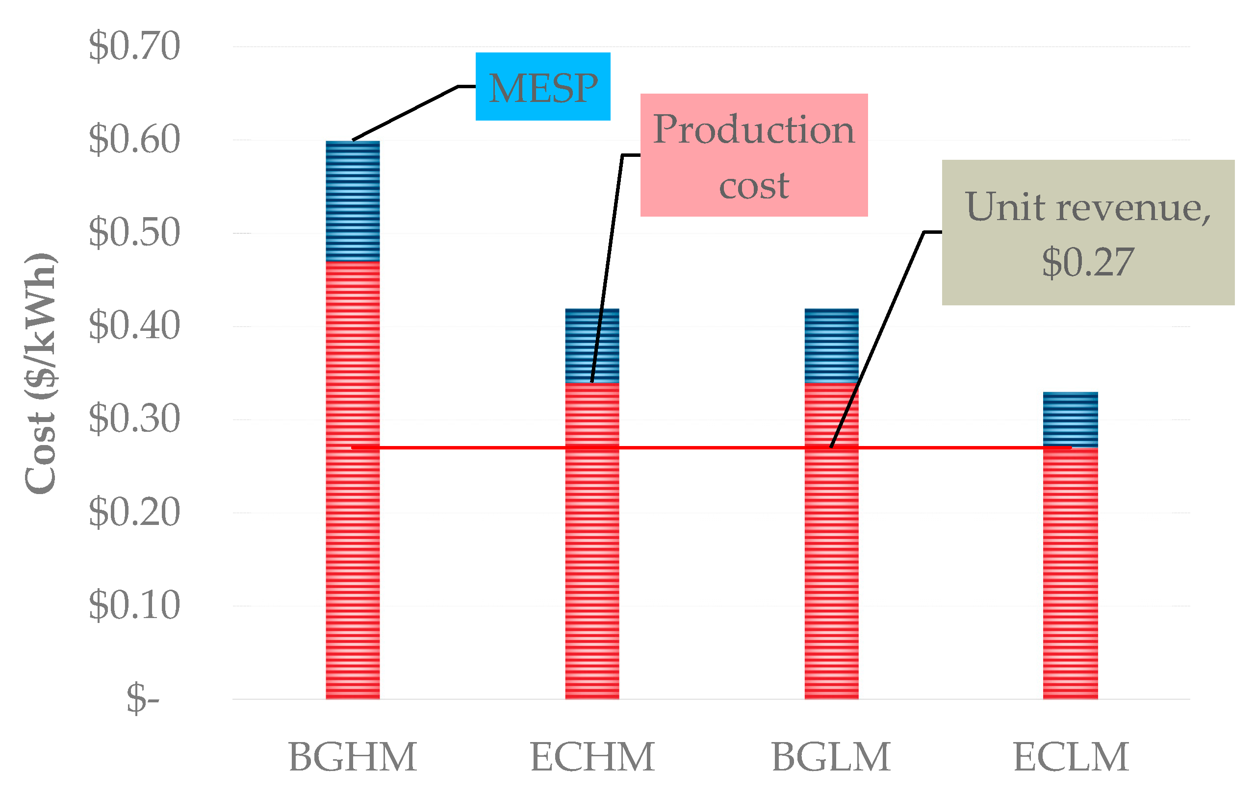
Figure 10.
A historical comparison of the unit cost of electricity, jet fuel, ethanol and ethylene in relation to crude oil from 2007 to 2016. The primary horizontal axis shows crude oil as $/L, while the secondary horizontal axis shows the crude oil as $/Barrel to ease understanding.
Figure 10.
A historical comparison of the unit cost of electricity, jet fuel, ethanol and ethylene in relation to crude oil from 2007 to 2016. The primary horizontal axis shows crude oil as $/L, while the secondary horizontal axis shows the crude oil as $/Barrel to ease understanding.


Table 1.
The composition of banagrass and energycane on a wet and dry basis.
| Composition | Banagrass | Energycane | ||
|---|---|---|---|---|
| Wet Basis | Dry Basis | Wet Basis | Dry Basis | |
| Cellulose | 10.22% | 37.48% | 10.05% | 33.44% |
| Hemicellulose | 6.39% | 23.43% | 6.36% | 21.16% |
| Lignin | 4.49% | 16.46% | 3.78% | 12.58% |
| Extractives | 3.56% | 13.05% | 7.92% | 26.36% |
| Ash | 2.61% | 9.57% | 1.94% | 6.46% |
| Moisture | 72.73% | - | 69.95% | - |
Table 2.
List of assumptions used in this study.
| Type | Assumption |
|---|---|
| Annual processing capacity | 60,000 dry MT/year |
| Biomass cost | $80/dry MT |
| Electricity cost | $0.27/kWh |
| Discount rate | 7% |
| Annual operational hours | 7920 h |
| Start-up time | 4 months |
| Construction period | 30 months |
| Income tax | 40% |
| Inflation | 4% |
| Project lifetime | 15 years |
| Depreciation method | Straight line |
| Salvage value | 5% |
| Depreciation years | 10 years |
Table 3.
The purchase cost of different equipment with their sizing data under different scenarios.
| High Moisture | Low Moisture | ||||||||
|---|---|---|---|---|---|---|---|---|---|
| BGHM Banagrass | ECHM Energycane | BGLM Banagrass | ECLM Energycane | ||||||
| Unit | Amount | Cost ($) | Amount | Cost ($) | Amount | Cost ($) | Amount | Cost ($) | |
| Conveyor belt | feet | 400 | 458,000 | 400 | 458,000 | 400 | 458,000 | 400 | 458,000 |
| Shredder | kg/h | 27,780 | 459,000 | 25,210 | 433,000 | 15,872 | 328,000 | 13,773 | 302,000 |
| Steam generator | kg/h | 29,635 | 372,000 | 42,048 | 485,000 | 41,585 | 481,000 | 53,607 | 583,000 |
| Expansion turbine | kW | 2591 | 590,000 | 3791 | 900,000 | 3747 | 892,000 | 4922 | 1,092,000 |
| Unlisted equipment | 470,000 | 569,000 | 540,000 | 610,000 | |||||
| Total cost ($) | 2,349,000 | 2,845,000 | 2,699,000 | 3,045,000 | |||||
Table 4.
Environmental impacts of different scenarios.
| Impact Category | Unit | High Moisture | Low Moisture | ||
|---|---|---|---|---|---|
| Banagrass | Energycane | Banagrass | Energycane | ||
| BGHM | ECHM | BGLM | ECLM | ||
| Acidification | kg SO2 equivalent | 3.0 × 10⁻³ | 1.2 × 10⁻³ | 1.9 × 10⁻³ | 9.3 × 10⁻⁴ |
| Eco-toxicity | CTUe | 1.2 × 10+0 | 5.5 × 10⁻¹ | 8.4 × 10⁻¹ | 4.1 × 10⁻¹ |
| Eutrophication | kg N equivalent | 8.1 × 10⁻⁴ | 4.1 × 10⁻⁴ | 5.3 × 10⁻⁴ | 3.0 × 10⁻⁴ |
| Global warming | kg CO2 equivalent | 2.9 × 10⁻² | 2.2 × 10⁻² | 1.9 × 10⁻² | 1.6 × 10⁻² |
| Carcinogenics | 1.3 × 10⁻⁸ | 9.7 × 10⁻⁹ | 8.8 × 10⁻⁹ | 7.2 × 10⁻⁹ | |
| Non-carcinogenics | 5.6 × 10⁻⁸ | 2.2 × 10⁻⁸ | 3.6 × 10⁻⁸ | 1.6 × 10⁻⁸ | |
| Ozone depletion | Kg CFC-11 equivalent | 7.1 × 10⁻⁸ | 2.6 × 10⁻⁸ | 4.6 × 10⁻⁸ | 1.9 × 10⁻⁸ |
| Photochemical ozone formation | kg O3 equivalent | 2.6 × 10⁻² | 2.8 × 10⁻² | 1.7 × 10⁻² | 2.1 × 10⁻² |
| Resource depletion | MJ surplus | 8.8 × 10⁻¹ | 2.3 × 10⁻¹ | 5.7 × 10⁻¹ | 1.7 × 10⁻¹ |
| Respiratory effects | kg PM 2.5 equivalent | 4.1 × 10⁻⁴ | 1.8 × 10⁻⁴ | 2.7 × 10⁻⁴ | 1.4 × 10⁻⁴ |
© 2017 by the author. Licensee MDPI, Basel, Switzerland. This article is an open access article distributed under the terms and conditions of the Creative Commons Attribution (CC BY) license (http://creativecommons.org/licenses/by/4.0/).
Share and Cite
MDPI and ACS Style
Rajendran, K. Effect of Moisture Content on Lignocellulosic Power Generation: Energy, Economic and Environmental Impacts. Processes 2017, 5, 78. https://doi.org/10.3390/pr5040078
AMA Style
Rajendran K. Effect of Moisture Content on Lignocellulosic Power Generation: Energy, Economic and Environmental Impacts. Processes. 2017; 5(4):78. https://doi.org/10.3390/pr5040078
Chicago/Turabian StyleRajendran, Karthik. 2017. "Effect of Moisture Content on Lignocellulosic Power Generation: Energy, Economic and Environmental Impacts" Processes 5, no. 4: 78. https://doi.org/10.3390/pr5040078
Note that from the first issue of 2016, this journal uses article numbers instead of page numbers. See further details here.