Article

Operator Training Simulator for an Industrial Bioethanol Plant

1
Biotechnology/IFM, Linköping University, 581 83 Linköping, Sweden
2
Lantmännen Reppe AB, 531 40 Lidköping, Sweden
3
Hochschule Furtwangen, University of Applied Sciences Furtwangen, 78054 Villingen-Schwenningen, Germany
*
Author to whom correspondence should be addressed.
Processes 2016, 4(4), 34; https://doi.org/10.3390/pr4040034
Submission received: 21 July 2016 / Revised: 4 September 2016 / Accepted: 9 September 2016 / Published: 22 September 2016

Abstract

:
Operator training simulators (OTS) are software tools for training process operators in large-scale industrial applications. Here, we describe the development, implementation and training of an OTS for a large-scale industrial plant for bioethanol production. The design of the OTS is based on conceptual analysis (previously reported by us in this journal) of various configuration alternatives and training procedures at the plant. In this article, we report on how the conceptual design is used in simulation models and graphical user interfaces and how the design is applied for training of operators in the real plant environment. The results imply that OTS would be time- and cost-efficient tools for application in the biotechnological industry.

1. Introduction

Operator training simulators (OTS) are software tools for training of operation procedures, troubleshooting, imparting fundamental process understanding, and maintaining and improving operational skills. A variety of OTS applications are found in airplane and sea pilot navigation, chemical manufacturing, and nuclear power production, as well as for military and surgery training [1,2,3,4,5,6,7,8,9,10,11,12,13].
Of particular interest for this study are OTS-applications in the chemical manufacturing industry. Examples are the use of OTS for training operators in process control [14], in operation of oil refineries [15], ammonia manufacturing [1], hydrocarbon manufacturing [15] and wastewater treatment plants [16]. Also of interest is the handling of accidents at chemical plants [10]. Training in the actual working environment with psychological factors in focus and with interaction in teams, either in the control room or by field operators, are mirrored by several authors [17,18,19,20].
In the biotechnological process industry, however, very few OTS have been realised, and they are limited to demonstrations with biogas, bioethanol and biopharmaceutical production in small-scale applications [21,22,23,24,25,26,27]. These previous studies have predominately been performed at a smaller laboratory scale in non-industrial environments or with only a single unit at a larger scale. They also do not show integrated process steps in bioethanol production plants or other bio-plants. However, although they do not describe and evaluate how the OTS are used in practice when used by operators in industry, they show the impact of OTS-based training in a variety of aspects. This article broadens this scope with examples from a large scale.
Operating training simulators use mathematical models capable of sufficiently simulating the real process in a realistic manner to allow efficient training in the virtual environment.
If this is successfully accomplished in bioprocess plant operations, several benefits can be foreseen, such as:
  • Time-efficient training of operators within a safe virtual environment
  • Rapid evaluation of operating concepts and procedures
  • Introduction of new operators to operational procedures
  • Reduction in time for start-up and shut-down due to better-trained operators
  • Increased operator skills in identifying faults and adjusting process parameters
  • Training of troubleshooting without compromising the real process.
The effectiveness of virtual training has been assessed by e.g., [3,28,29,30,31] as well as in previous bioprocess-related studies by us [23,24,25,26]. These assessments all conclude that the transfer-of-training factor, i.e., how efficient the OTS is in developing understanding, skills and other capacities of the trainee as a result of the training [3,6], is high and supports the use of OTS in academic as well as industrial training. Several detailed assessment procedures have been applied as reported by these authors and others [19,20,21]. However, observations of effects are more complicated to perform when OTS are applied in industrial environments, such as in a whole complex plant with a large number of process units operated by comparatively small groups of operators.
This article describes the development and training experiences of an OTS for a large-scale bioethanol plant. The design of the OTS and the structure of the training are based on a conceptual design study, previously performed by us, where key requirements and constraints were precisely defined [32]. The implementation of user-friendly graphical user interfaces (GUIs), with a high degree of resemblance with the real control room environment, and mathematical models describing the unit operations of the plant, are presented. Experiences from using the OTS in a large-scale plant environment are shared and practical examples highlight typical training features of the OTS.

2. Materials and Methods

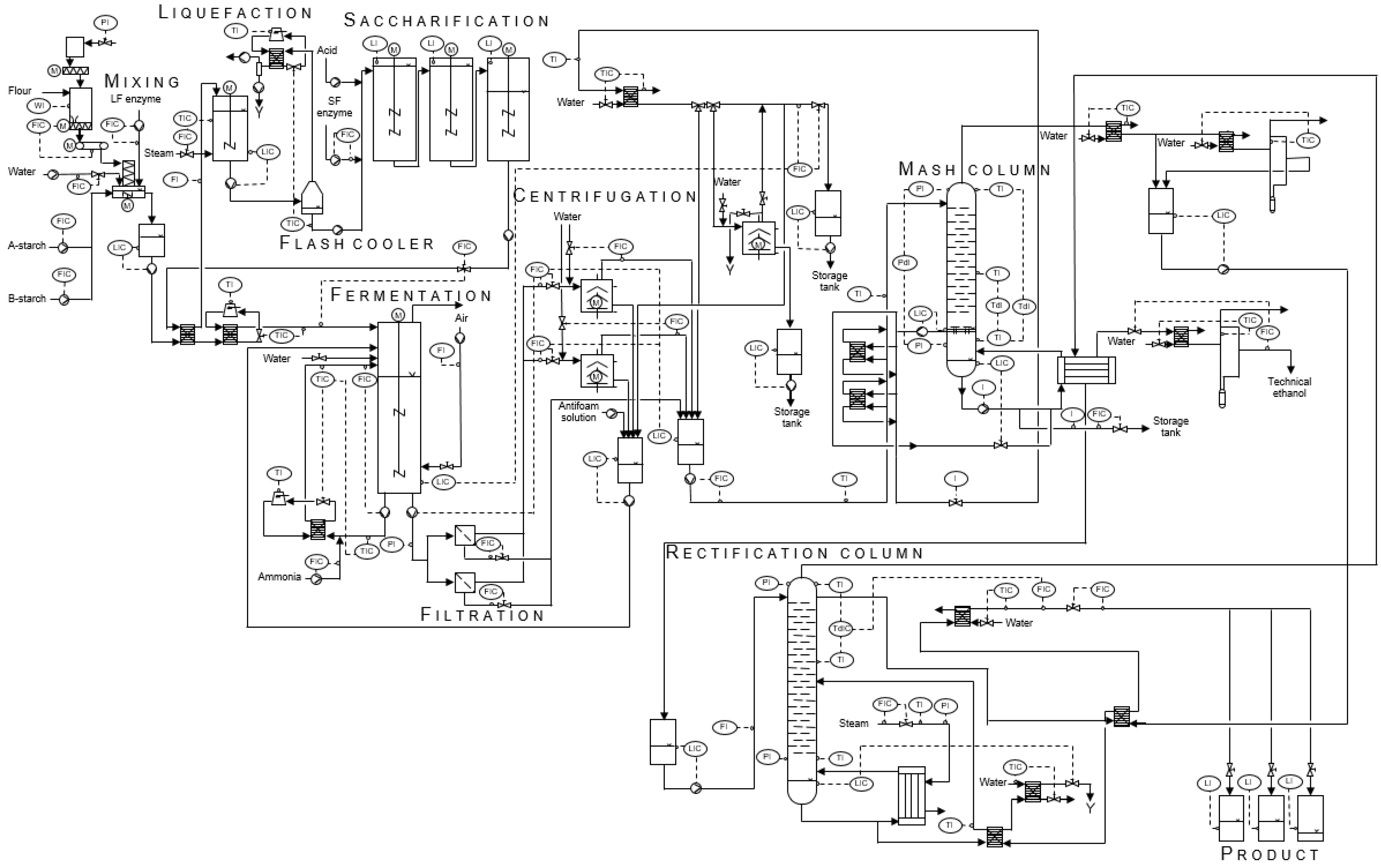
2.1. The Bioethanol Plant

The OTS was developed for operator training at a large-scale bioethanol plant (Lantmännen Reppe AB). The plant, situated in Lidköping (Sweden), is operated according to the Biostil method for continuous ethanol production (Chematur Engineering AB, Karlskoga, Sweden, [33]). In the plant, wheat is converted primarily to potable ethanol, but also dried and modified starch, vital wheat gluten, glucose syrup and raw ingredients for animal food are produced as side products.
Figure 1 depicts the ethanol production line of the plant structured into five sections:
  • A pretreatment section, for mixing of the cereal raw materials
  • A hydrolysis section, for liquefaction and saccharification
  • A fermentation section, for conversion of glucose to ethanol by a commercial yeast strain
  • A separation section, using filtration and centrifugation
  • A distillation section, including one mash and one rectification column.
Cooling of the liquefaction outflow is achieved by applying a vacuum pump system (FLASH cooler). A filtration system separates fibre mass from the broth. Yeast cells are subsequently separated by two centrifuges. The heavy liquid including cell mass and solids is transferred to a tank from which the liquid is recycled to the fermenter while light liquid is transferred to a tank that is connected to the distillery. A third centrifuge is used to recycle the return bottom fraction from the mash column. At the top of the mash column ethanol vapour is removed, cooled and transferred to the rectification column where the ethanol-water mixture is further distilled to ethanol to a concentration of approximately 96% (v/v).

2.2. Simulation Software

The OTS was developed and implemented in the process control and automation system WinErs (version 6.3A, Ingenieurbüro Dr.-Ing. Schoop GmbH, Hamburg, Germany, [34]). COM-interface blocks provided connections for external software communication. All models were implemented as dynamic link libraries (DLLs) (Visual Basic, C, C++, Delphi). Mathematical models were programmed in C++ with the compilation tool eStIM-C++ (University of Applied Sciences, Bremen, Germany). Dynamic simulations were performed using coupled non-linear differential and algebraic equations. A Runge-Kutta-algorithm was applied to solve differential equations in WinErs. A PC with 4 GB RAM and a dual- or quad-core CPU was used to run the software.

3. Results and Discussion

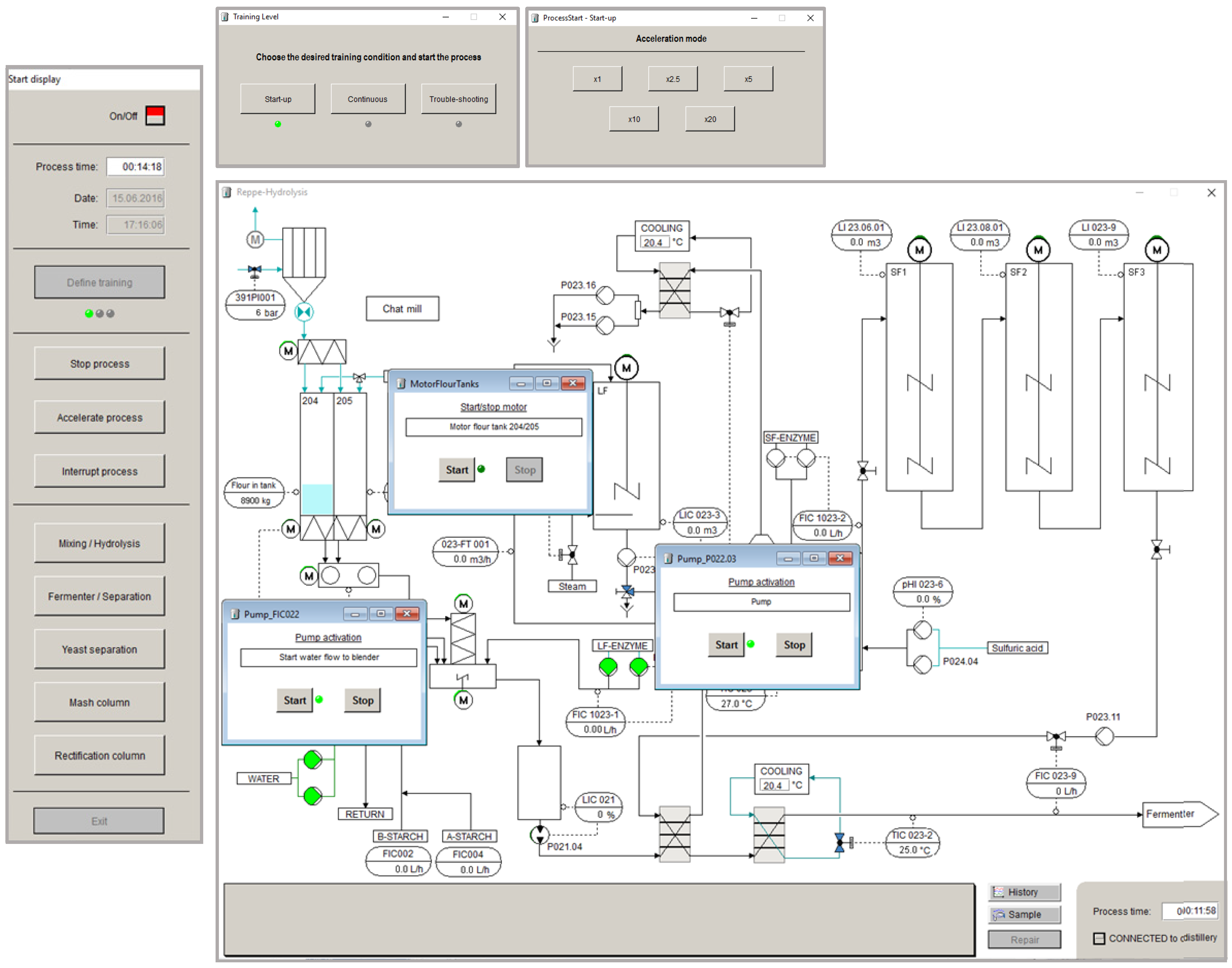
3.1. Strategy for Development of OTS

In a previous work we applied conceptual design methodology for defining the ideal structure of the OTS for the bioethanol plant [32]. The structure and the procedure for training were established based on needs expressed by the plant’s management and experienced operators. These needs were:
  • Support existing training procedures at the plant for increasing training efficiency and decrease training time
  • Exploit the possibility of accelerating real process time in the simulation to enhance time-efficient training
  • Allow training of existing standard operating procedures (SOPs) at the plant
  • Allow training of start-up and shut-down procedures without interfering with the real process
  • Allow training of typical troubleshooting events and incident situations occurring at the plant
The needs guided the development and implementation of the graphical user interfaces (GUIs), simulation model framework and operator training procedures of the OTS prototype.
Critical steps in the implementation were to ensure that the GUIs showed a high degree of correspondence with the GUIs in the control room at the plant. Also important was that the distributed control systems (DCS) were correctly displayed in these GUIs. Another critical step was to ensure that the implemented models allowed realistic and robust simulations at the range of operating conditions occurring during continuous operation, start-up, shut-down and typical incidents at the plant or common operator failures. Moreover, simulation of equipment, instrumentation and control loops should be as realistic as possible. Particular attention was also paid to model accuracy, accelerated process time and ability of the memory capacity of the computer to simulate the virtual process over extended time periods. In the following is described how the GUIs, the models and other computational procedures were implemented and tested and, finally, how the OTS prototype could be used in the training at the plant.

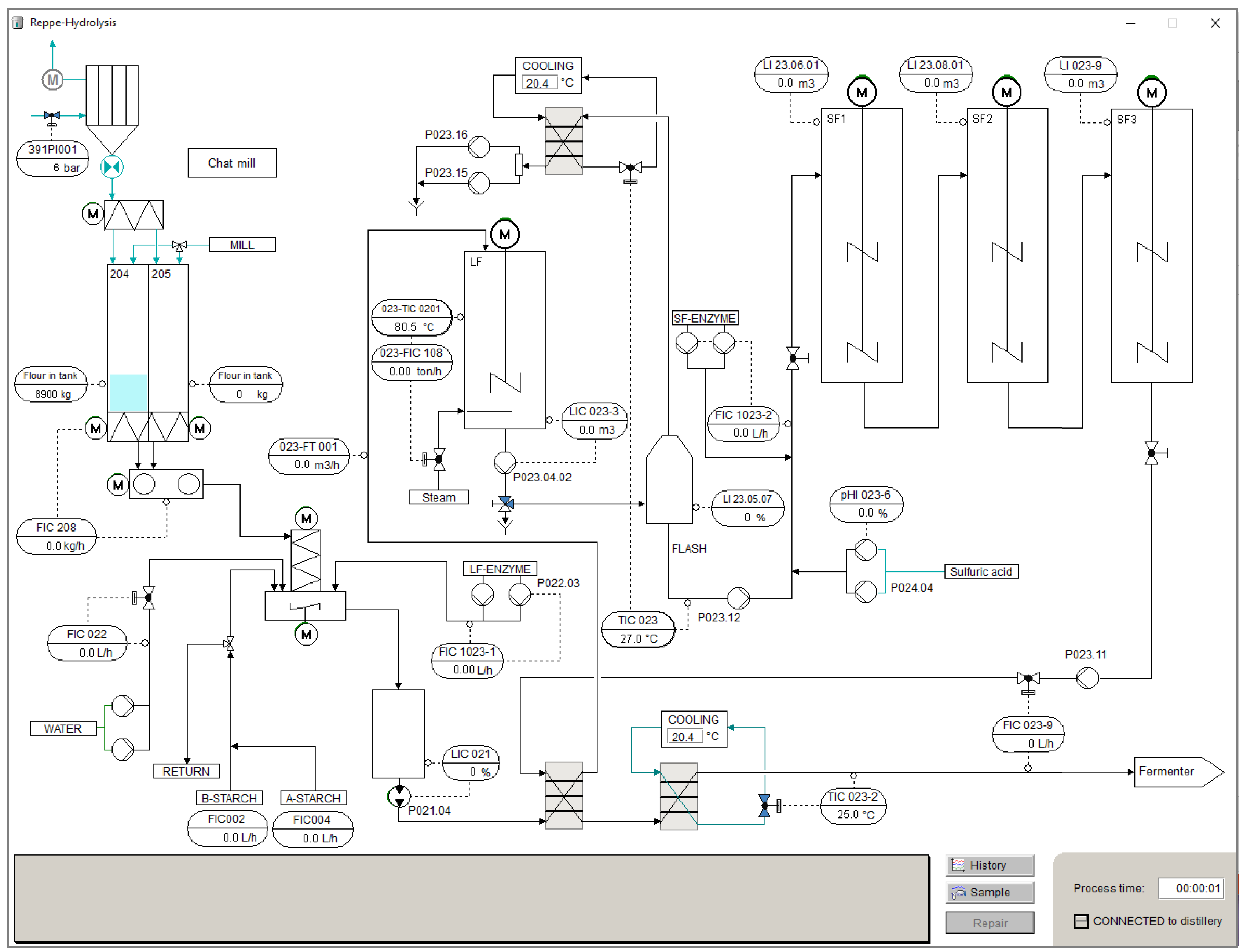
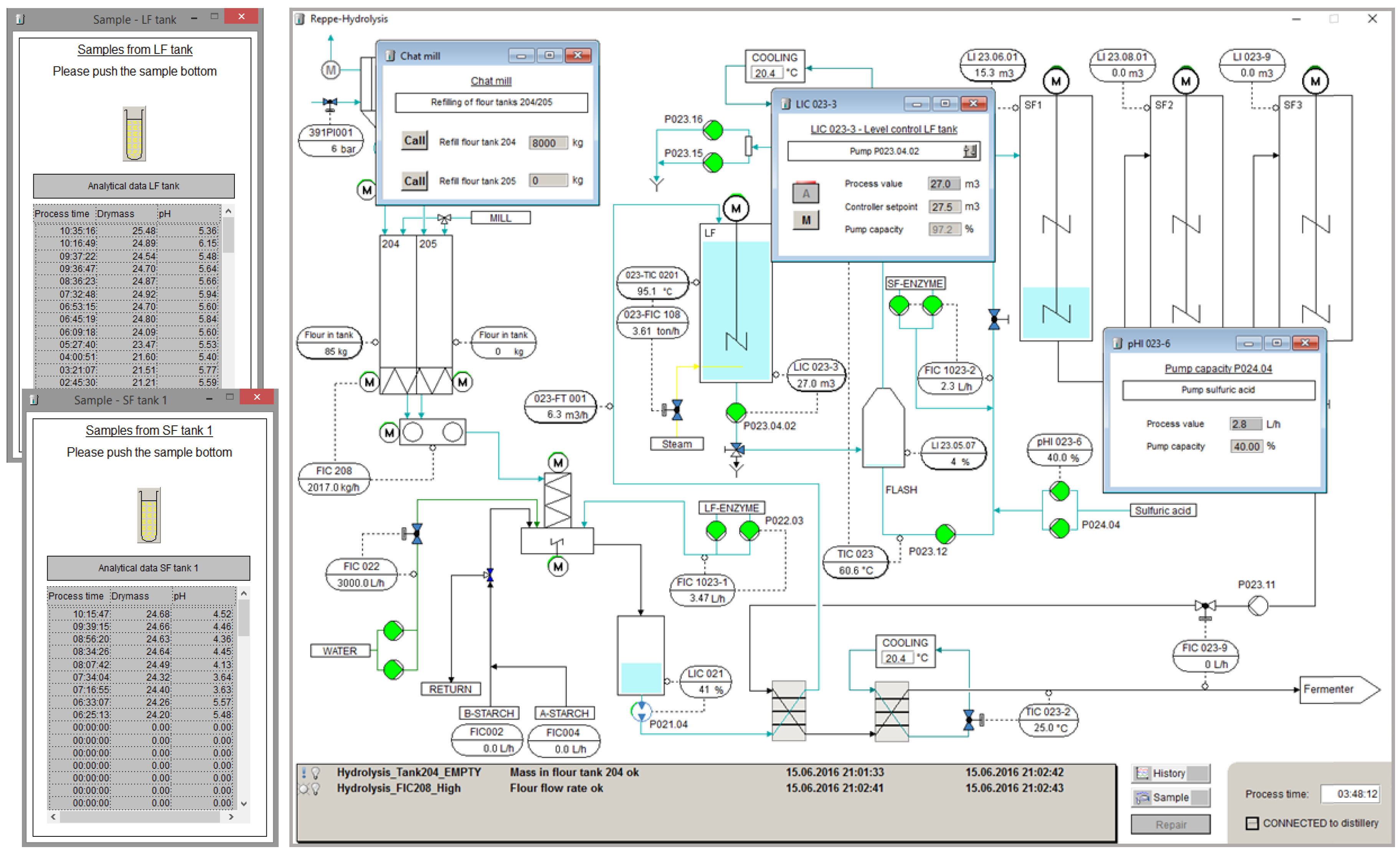
3.2. Graphical User Interfaces

The design and implementation of the GUIs of the OTS are decisive for ensuring an efficient transfer-of-training effect. Critical is the resemblance of the OTS with the real operator environment and in particular the process flow diagrams of the GUIs used in the control room of the plant [2,24,35,36]. This was generally the case with few exceptions in this study.
Figure 2 shows the GUI of the hydrolysis section, including the pre-treatment section (mixing) where flour is provided from the mill and blended with water and enzymes in subsequent tanks. Enzymatic hydrolysis takes place in one liquefaction tank, a flash cooler tank and three saccharification tanks. Three heat exchangers ensure cooling. The GUIs for the other sections of the plant are provided in the Supplementary Materials (Figures S1–S4).
The presented GUIs resemble the GUIs of a real plant control system with high fidelity. Process diagrams, controllers, motor and pump functions are available via sub-windows. This setup of GUIs shall enhance a realistic training and an effective transfer of training. In addition, the GUIs depict the virtual process time and allow manual sampling via sub-windows.
Furthermore, a start display allows the user to define the training by choosing start-up or continuous mode and acceleration time (1-, 2.5-, 5-, 10- and 20-fold). In order to visualise process values such as temperatures, volumes and flow rates on the GUIs’ relevant signals were defined and linked with the interfaces. Moreover, signal inputs that can be defined by the trainee must be available and changeable via the GUIs. These signals might be outputs from a model that are directly revealed on the interface (e.g., volume, temperature) or input values that are defined by the trainee (e.g., adjusting a flow rate, changing a controller set point) and that are linked to the models.
Also, these signals might be intermediate outputs where a model output is further computed. For instance, the model output for a volume of a tank is given in (m3) while the GUI visualises the volume in (%), or, in order to implement sampling procedures, the concentrations of the components coming from the models are further computed to a dry weight (% w/w) that is shown on an additional sub-window for sampling. These intermediate outputs enhance the training effectiveness because they better represent the real system.
Several elements on the GUIs are animated to better reveal what pipe or instrument is active (e.g., by a change in colour of a pipe or pump). Also, alarm messages, for instance when an actual pump rate deviates from the controller set point, is shown to the operator during a virtual process. This trains the operator’s capability to recognize faults and non-standard conditions immediately.

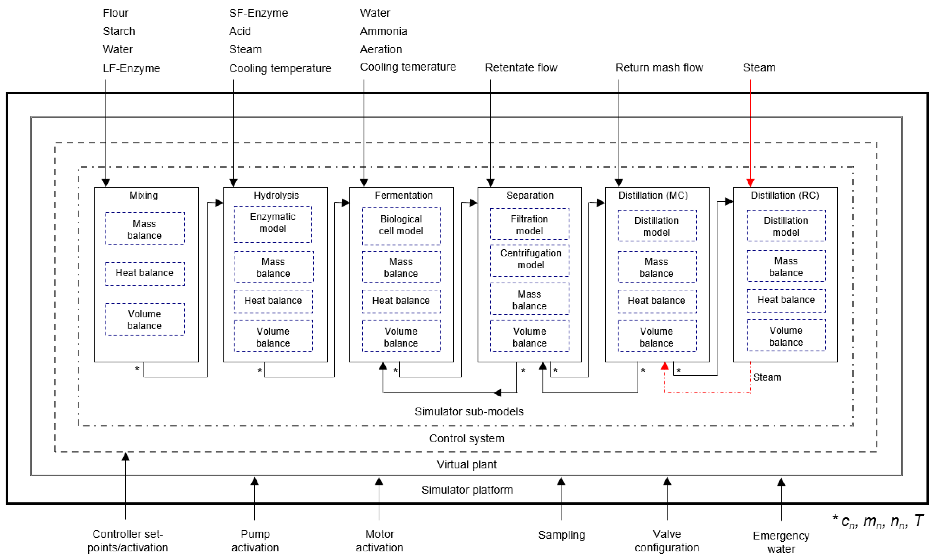
3.3. Modelling Framework of the Simulator

A framework of simulation models for unit operations of the bio-plant was derived from established first-principle engineering models [37,38]. The specific user needs we previously identified [32] guided the selection of models and other equations in the framework. These models were partly modified and adapted in order to allow dynamic simulation under standard, start-up, shut-down and other critical conditions.
Adaption of the model parameters to the real plant is crucial. The better the model parameters, such as enzyme and cell kinetics, are tuned, the more comparable the operating values become. Furthermore, high model accuracy and robustness [35,36,39,40,41] are required in order to allow effective training at critical conditions such as starting a centrifuge, emptying tanks or controller malfunctions.
All process parameters were collected from literature and our own data. Each of the process sections with its key units was modelled and included:
  • Pre-treatment (general tank model for mixing of components)
  • Hydrolysis of starch (including liquefaction, saccharification, flash cooler and heat exchangers)
  • Fermentation of glucose to ethanol by yeast cells (including heat exchanger)
  • Separation of yeast and return mash (including filtration and centrifugation as well as intermediate tanks)
  • Distillation of the broth in the mash column to approximately 40% (v/v) ethanol (including heat exchangers and intermediate tanks)
  • Distillation of the distillate in the rectification column to approximately 96% (v/v) ethanol (including heat exchangers as well as intermediate and product tanks).
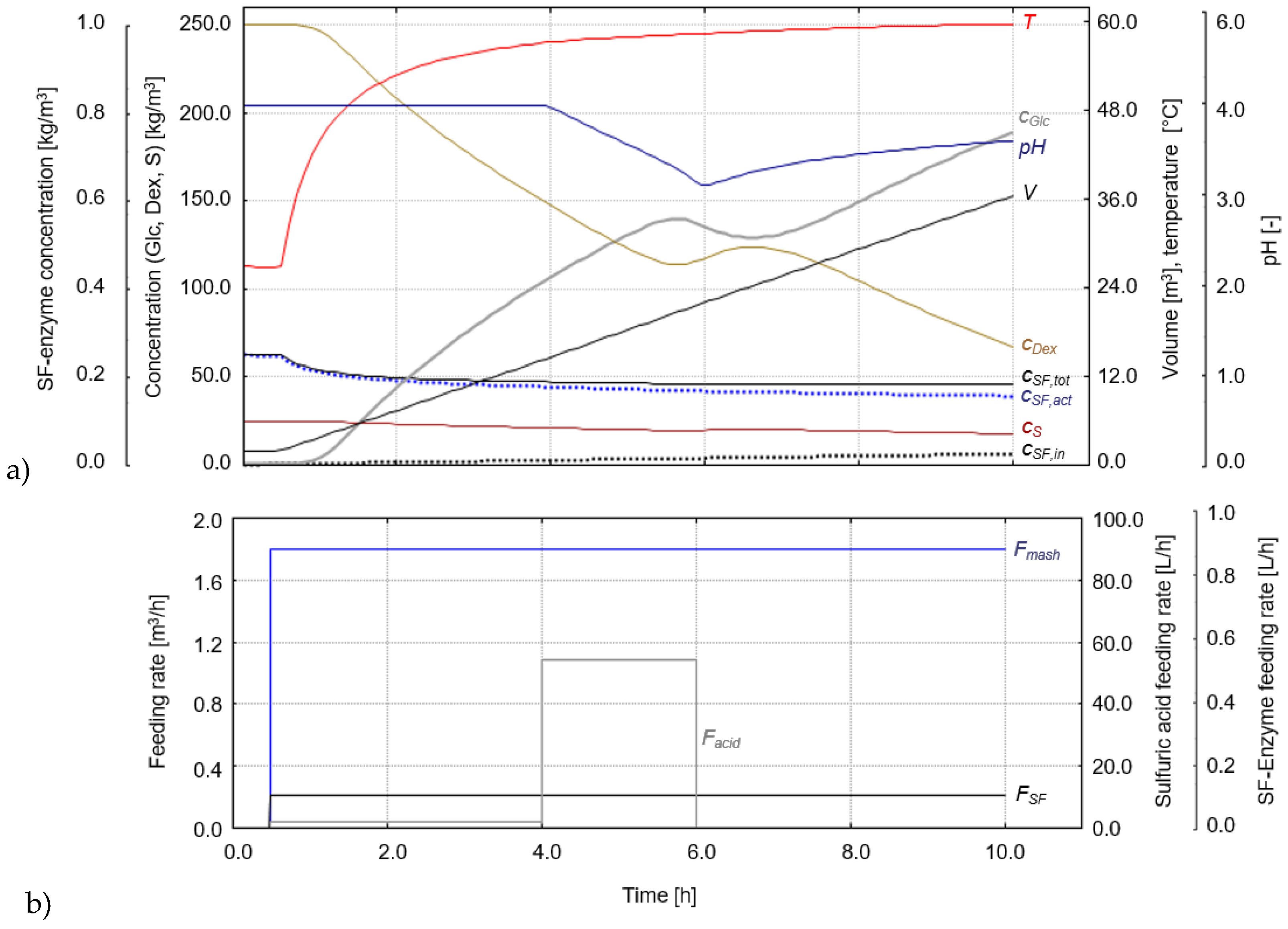
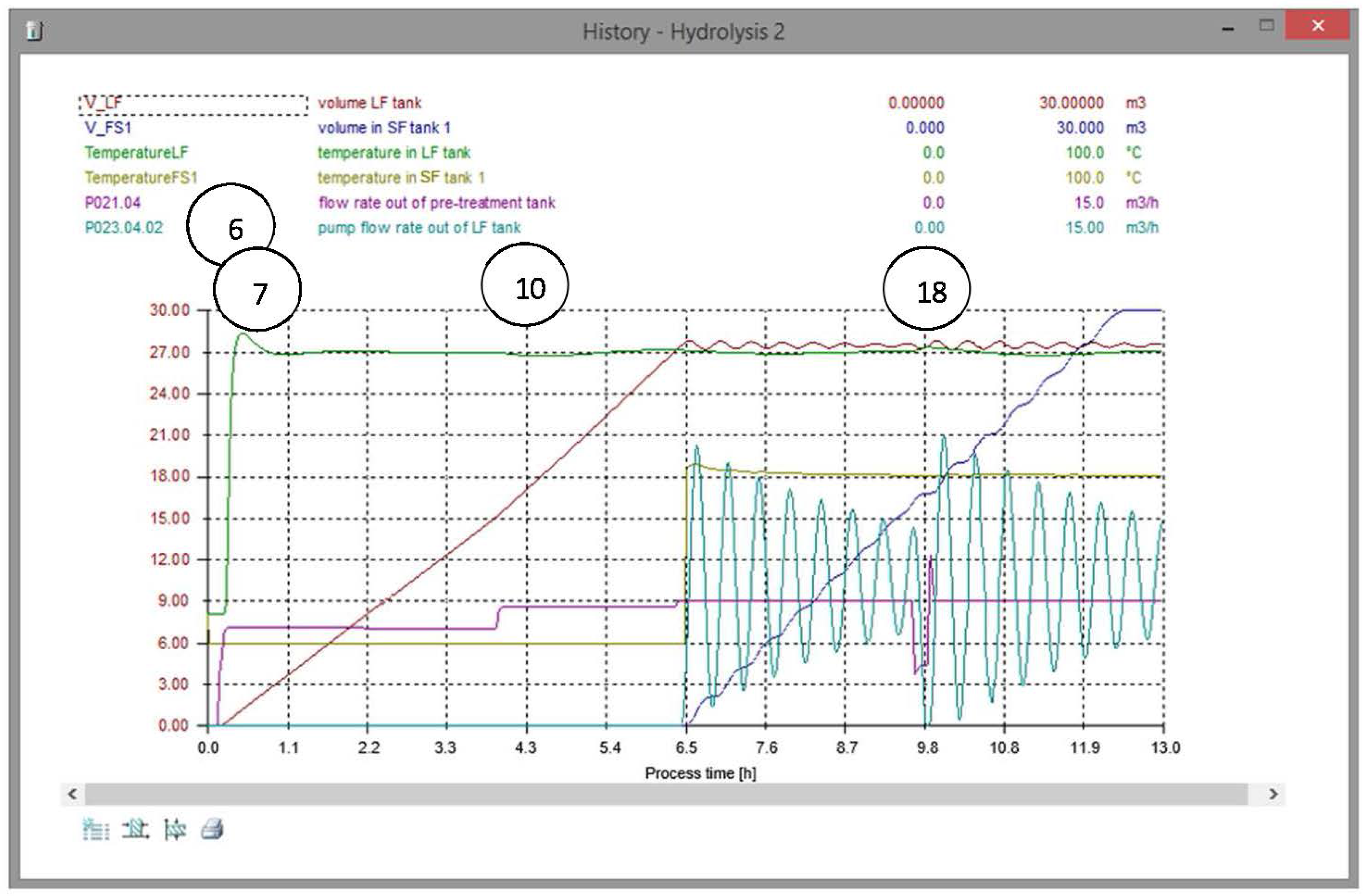
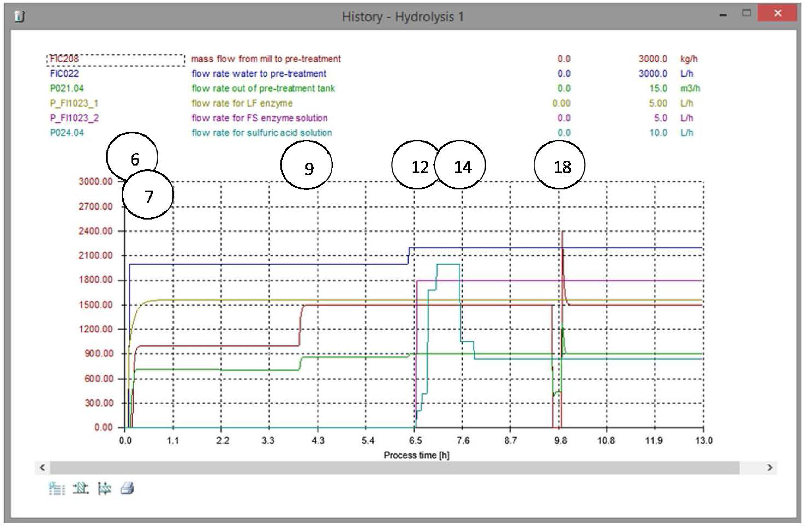
Figure 3 shows a simplified shell structure of the model framework, separated into kinetic and dynamic sub-models. The model framework includes sub-models for physico-chemical and biological reactions describing the fermenter, filter and centrifuges, sub-models for equipment, such as pumps, valves and heat exchangers, and sub-models for the distributed control systems (DCS) of the plant. Input parameters are given by the trainee or to the virtual plant such as activation of pumps, motors and controllers affecting the models that are further computed.
Model simulation results are shown for the hydrolysis and separation sections, in particular centrifugation to exemplify the applicability of the models for operator training. An overview of the state variables used for each sub-model is provided in Table S1 (Supplementary Materials).

3.3.1. Hydrolysis

To simulate the course of a hydrolysis process in the OTS, a model is described following the principles of previous work [23,24,25,26].
The enzymatic reactions can be expressed using stoichiometric equations with stoichiometric coefficients n and x for [42,43]:
Dextrins from starch:
( C 6 H 10 O 5 ) n + n ( H 2 O ) x ( C 6 H 12 O 6 ) n / x
Glucose from starch:
( C 6 H 10 O 5 ) n + n ( H 2 O ) n ( C 6 H 12 O 6 )
Glucose from dextrins:
( C 6 H 10 O 5 ) n / x + n x ( H 2 O ) n x ( C 6 H 12 O 6 )
In the liquefaction tank α-amylase (LF-enzyme) converts starch to intermediate sugars (i.e., dextrins, oligosaccharides and disaccharides). The conversion rate is limited by the starch concentration (cS,LF) by using Michaelis-Menten kinetics.
In our previous work, a double sigmoidal function [24] was developed showing how dynamic changes of enzymatic and metabolic changes can be simulated in an OTS. Here, the sigmoidal function is used to describe dynamically the dependence of the activity on dry mass (DM), temperature (T) and pH:
q Dex / S , LF = k Dex / S , LF · c S , LF ( c S , LF + K S ) · c LFact c LF , tot · y ( D M LF ) · y ( T LF ) · y ( p H LF )
where kDex/S,LF is the maximum conversion rate for LF-enzyme [kg·kg−1·s−1] and KS the Michaelis-Menten constant [kg·m−3]. The reaction is catalysed by the active LF-enzyme (cLF,act) where the rate is given by the ratio of active LF-enzyme to total LF-enzyme concentration. Total LF-enzyme concentration is the sum of active and inactive LF-enzyme concentration. The concentration of inactive enzyme is used to model activity loss due to denaturation caused by temperature and pH. For instance, when a certain amount of active enzyme is irreversibly inactivated (cLF,actcLF,in), the activity decreases while the total amount of enzyme is maintained. The interaction between active and inactive compartments is also applied in the cell metabolism (fermentation sub-model) as previously shown [25]. Model outputs for starch, dextrins, glucose, non-hydrolysable components, such as proteins and fibres, are used to compute the dry mass.
In the saccharification process, glucoamylase (SF-enzyme) is added to convert dextrins to glucose. The same model principle is applied for all enzymatic reactions Equations (1)–(3). Using the stoichiometric coefficients and molecular weights (MW) of the components’ specific formation rates for dextrins from starch as well as glucose from starch and dextrins [kg·kg−1·s−1] are:
q dex = x · M W Dex · n x M W S · n · q Dex / S
q glc = n · M W Glc M W S · n · q Glc / S
q glc = n x · M W Glc M W Dex · n x · q Glc / Dex
Mass balance equations and reactions allow dynamic simulation in the OTS:
d c i d t = q i + · c En , tot · q i · c En , tot + c i feed · F c i V · c i · F t o t V
where c i is the concentration of starch, dextrins or glucose respectively [kg·m3], q i + / q i the formation rate and conversion rate [s−1]. Concentration of total enzyme is expressed as c E n , t o t (En: LF or SF) and of starch, dextrins and glucose in the feeding solution as c i f e e d [kg·m3]. F t o t is the total volumetric feed rate [m3·s−1] and V the volume [m3].
Simulation results for a fed-batch reactor where dextrins are converted to glucose by the SF-enzyme and the corresponding action of the operator are shown in Figure 4.
Figure 4a shows how enzymatic activity is affected by temperature and pH due to the integration of double sigmoidal function values Equation (4). In Figure 4b, it is shown how the operator after 1 h starts feeding at 1.8 m3·h−1 (Fmash) (feed temperature: 60 °C). The feeding solution has the same concentrations of starch, dextrins and glucose as shown for the initial values. The operator adds SF-enzyme solution at a feed rate of 1.1 L·h−1 (FSF) and acid at 1.9 L·h−1 (Facid). With increasing temperature, the activity increases. At 4 h, the operator increases the acid flow rate to 54 L·h−1 causing a decrease of the pH affecting enzyme activity. After 6 h, the operator stops acid feed to adjust the pH. Activity loss by inactivation of active to inactive SF-enzyme is also shown. Both form the total mass of enzyme in the tank (cSF,tot). In OTS training, the trainee is supposed to adjust the pump speed for acid manually to ensure optimal conditions. Also, the trainee must set appropriate initial feed rates for enzyme solution, water, flour and starch. The model is able to react dynamically to the operator’s control actions.

3.3.2. Fermentation

The fermentation sub-model of the OTS consists of a biological cell model embedded in an ideal stirred reactor model. The fermentation model is based on a structured model that includes compartments for active, structural, inactive and dead biomass for describing the cell metabolism under aerobic and anaerobic conditions [25]. Substrate uptake rates for glucose, ammonia and ethanol (diauxic growth) are modelled by Michaelis-Menten kinetics. Reactions are catalysed by the active biomass ( X a c t ) compartment:
q G = q G , max · c G c G + K G · c Xact c Xv · y ( D O ) · y ( c E t O H ) · y ( c N H 3 ) · y ( c G ) · y ( p H ) · y ( T M )
where q G , max is the maximum glucose uptake rate, K G the Michaelis-Menten constant and Xv the total biomass.
Double sigmoidal functions were applied in the model and revealed the feasibility to dynamically simulate changes in cell metabolism and substrate flux based on dissolved oxygen (DO), ethanol (EtOH), ammonia (NH3), glucose (G), pH and temperature (TM). For instance, the switch from aerobic to anaerobic metabolism is modelled using DO as argument x of the sigmoidal function.
Using stoichiometric equations, the formation of biomass, ethanol, carbon dioxide and side-products (here water only) as well as oxygen consumption from glucose (G) and ethanol (EtOH) are described according to:
C 6 H 12 O 6 + j O 2 , X / G O 2 j X / G CH 1 . 8 O 0 . 6 + j CO 2 , X / G CO 2 + j H 2 O , X / G H 2 O
C 6 H 12 O 6 + j O 2 , EtOH / G O 2 j EtOH / G C 2 H 5 OH + j CO 2 , EtOH / G CO 2 + j H 2 O , EtOH / G H 2 O
C 2 H 5 OH + j O 2 , X / EtOH O 2 j X / EtOH CH 2 O 0 . 6 + j CO 2 , X / EtOH CO 2 + j H 2 O , X / EtOH H 2 O
Specific growth rates for the biomass compartments as well as consumption and production rates are obtained from stoichiometric equations with glucose, ammonia and ethanol as substrate. The respective fluxes to the biomass, ethanol and energy formation pathway are used in mass balance equations according to Equation (8).

3.3.3. Filtration

The separation section of the OTS uses two filtration and three centrifugation equations.
In the filtration units of the plant the inflow from the fermenter and the retentate and permeate outflows are balanced. Fibres in the retentate flow are separated while smaller particles (≤200 µm), such as cells and starch, are transferred to the centrifuges. Under standard operation conditions the retentate flow rate is 30-fold lower than the permeate flow rate. An important process parameter in OTS training is the pressure before and after the filter on the permeate side. General filtration theory is here used to describe the transmembrane pressure and its influence on the permeate flow [44]:
Δ p = p i + p 0 2
where pi is the membrane feed inlet, p0 the outlet pressure (retentate) and pP the pressure on the permeate side.
By starting the inflow pump to the filter unit, the inlet pressure across the membrane increases (to a value characteristic for the plant). With increasing retentate flow also the transmembrane pressure increases. The maximum permeate flow rate is calculated as:
V p e r = Δ p · A μ f   [ α · ( M c A ) + R m ]
where A is the filter area [m2], μ f the filtrate viscosity [kg·m−2·s−1], M c the total mass of solids in the filter cake [kg], α the average specific cake resistance [L·Mc−1], and R m the filter medium resistance [L−1].

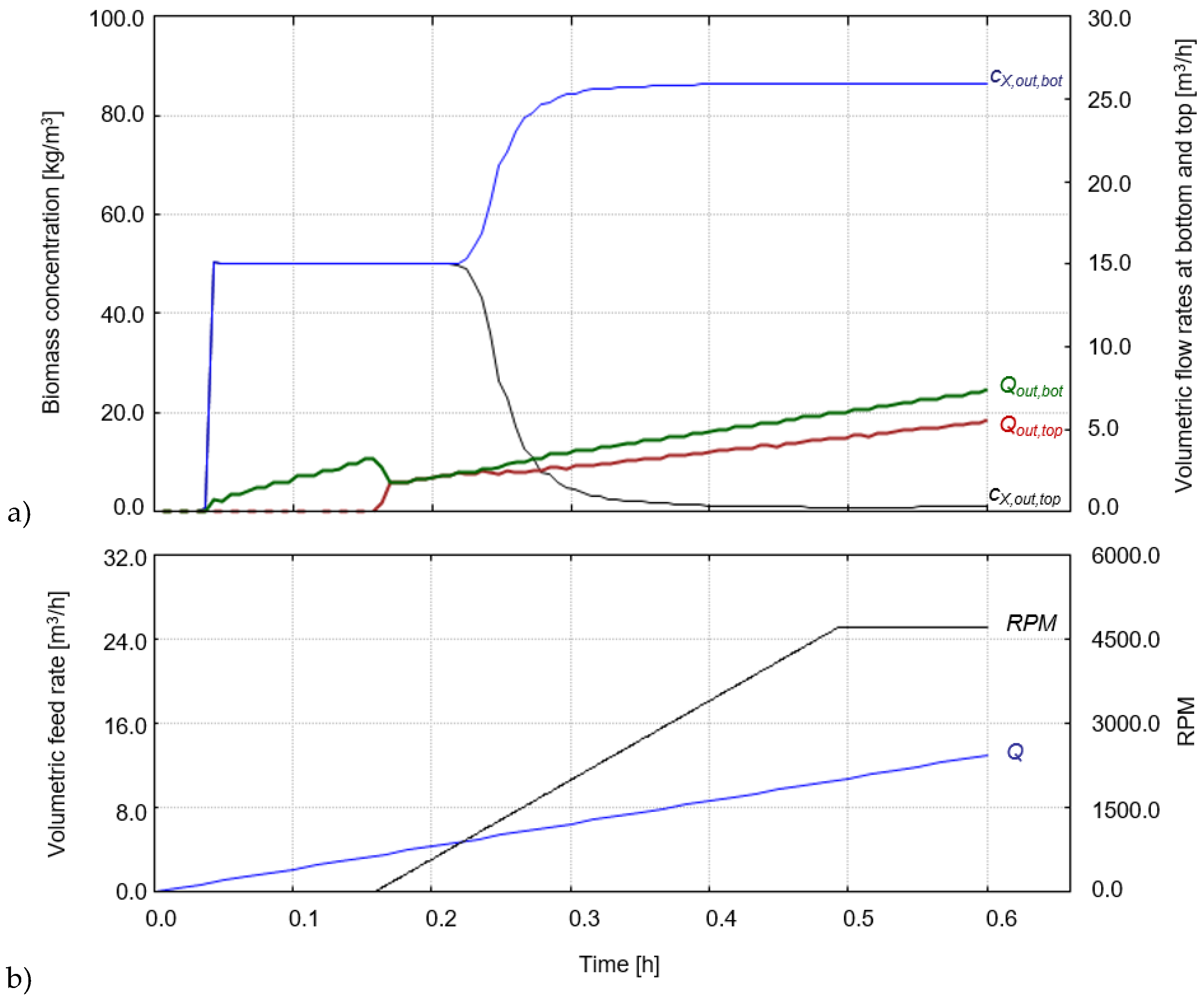
3.3.4. Centrifugation

Inflow rates to the centrifuges depend on the computed permeate flow rate. The inflow rates are adjusted by the opening degree of the valves before the centrifuge inlets, where the computed permeate flow rate is the maximum value.
The total mass of solids is described by the mass of fibres in the filter assuming that a certain amount of the fibres mass (dmFi/dt) forms the filter cake. A stirrer inside the filter unit ensures that the outlet flows are homogeneous. If the stirrer is interrupted, accumulation of fibres occurs and the retentate and permeate flows decrease or stop. This was implemented in the troubleshooting training in the OTS.
Concentrations of each component in the broth in the retentate and permeate are then computed. Here, it is assumed that the concentrations of dissolved components (including ethanol), as well as of starch, non-hydrolysable components and biomass remain unchanged in the volumetric flow of the retentate and permeate while the mass of fibres may change in the retentate flow.
The equations for centrifugation in the OTS describe the mechanism of a disc stack centrifuge of the types used in the bioethanol plant where cells or biomass (also return mash) are discharged continuously. Established centrifuge equations [44,45,46] were adapted and implemented in the OTS for allowing dynamic simulation of yeast separation.
The following set of equations were used in the OTS:
The angular velocity of the bowl [rad·s−1] for cell recovery is:
ω Rec = 2 · π · S Rec ( 1 9.55 )
where SRec defines the rotation speed [rpm] for adjusting the recovery factor (yRec(υP)) Equation (19).
The ∑-factor [m2] for disk centrifuges is used as performance parameter for comparing the cell recovery for different centrifuge sizes:
Rec = 2 · π · ( ω Rec ) 2 · ( N 1 ) 3 · g · tan θ   ( r out 3 r in 3 )
where N is the number of discs [-], rout [m] the outer radius of the disc and rin [m] the inner radius of the disc and θ the half of the cone angle of the disc [-].
The ∑-factor is independent of the properties of the fluid and particles and depends on size of the centrifuge and the rotation speed.
By using the ∑-factor [m2] and volumetric feed rate [m3·s−1] the sedimentation velocities for cell recovery (υRec) and the actual process values (υP) are computed as:
υ Rec = ( Q Rec · f Q Rec ) · f υ
υ P = ( Q · f Q ) · f υ
Model adjustments were done using the parameters fQ and fʋ. From that the recovery factor yRecP) and the yield for recovered cell mass (%) is defined as:
Y Re c = 100 · y Re c ( υ P )
where yRecP) is calculated using the sigmoidal function where υ P is the argument x of the function while υRec is applied as reference value (1.0 < yRec ≥ 0.5). A high cell recovery yield is achieved when υRec = υP. Online signals on the plant showed that, when the rotational speed is below 50 rpm, there is only an outflow at the bottom of the centrifuges. This was also implemented in the OTS. The outflows for heavy (bottom) and light liquid (top) under running conditions are further computed. Concentrations for dissolved components are unchanged in each of the volumetric outflows while cell mass (mX,out,n; expressed in kg·h−1) is separated based on YRec:
m X , out , bot = Q · c X feed · Y Rec 100
m X , out , top = Q · c X feed ( 100 Y Re c ) 100
Using Equation (20) as well as the incoming broth and water flow, the volumetric outflow [m3·s−1] is calculated:
Q out , bot = ( Q Q X ) + Q water + m X , out , bot ρ X
where QX is the volumetric feed rate formed by the cells and ρ X the cell density. The same is applied for the outflow at the top of the centrifuge.
From that, the cell concentration in the outflow at the bottom of the centrifuge is:
Q out , bot = Q Q X 2 + m X , out , bot ρ X
Figure 5 shows a simulation of the start-up procedure of the centrifuge in the OTS using a biomass concentration in the feed of 50 kg·m−3.
The operator starts the volumetric feed rate to the centrifuge (Q), gradually increasing to 13 m3·h−1. At 0.15 h, the operator starts the centrifuge and the rotational speed is gradually increased to 4700 rpm. When the rotational speed reaches 50 rpm, liquid flows out at the top as well as the bottom (Qout,top and Qout,bot). After 0.2 h, the biomass concentration in the outflow at the bottom (cX,out,bot) increases while the concentration at the top (cX,out,top) decreases. The simulation shows how the rotational speed affects the separation efficiency. Notably, (Qout,bot) increases with increasing biomass concentration, showing the effect of separation where the outflow with cells has a higher volume and density than without cells. Thus, the results show that detailed modelling of the yield of recovered cell mass and volumetric outflows was required to allow dynamic simulation of start-up or shut-down procedures in the OTS training.

3.3.5. Distillation

Two distillation sub-models, previously applied in a training simulator [27,47], were used. These models describe the molar balance of water and ethanol as well as the heat balances for the mash column (MC) and rectification column (RC). However, since ethanol distillation has previously been described in detail for OTS applications, focus has here been of the upstream parts of the bioethanol process.

3.4. Experiences of Training with the OTS

Observations of effects when OTS are applied in industrial environments such as a whole plant with a large number of process units, sensors, actuators and other devices are, from a scientific methodology perspective, cumbersome. The time for running training of operators at a plant typically extends over long periods. Possibilities to observe cause-and-effect relations are therefore more difficult compared to laboratory-scale studies with lesser units, shorter training periods and better control of the experimental situation (cf. [19,20,21,24,25,26]).
In this study, the OTS prototype was assessed with newly employed operators with minor experience of working at a bio-plant for a period of three months. The assessment was divided into three parts. The first part comprised observation of operator behaviour based on a list of events, actions or cause and effects that the study leaders identified beforehand. The second part in the assessment was to observe and record unexpected operator behaviours not listed beforehand. The third part was to analyse all observations, compare these over time and draw conclusions. Observed effects and other notations were all documented. The assessment training was supervised by experienced operators and plant engineers. Also, the training procedure mirrored our previous study of design of the training at the plant [32].
Table 1 provides a collection of examples of typical observations of performance of operation procedures, failures and mistakes caused by the operators.
The most striking observation was that the simulator training was an effective method to train the sequential actions in the standard operation procedures (SOPs). The simulator animated the procedures and recorded and displayed deviations with a high degree of fidelity to the real plant. The effects of the operators’ actions were immediately and correctly visualised on the GUIs of the simulator and allowed corrective actions by trained operators themselves, or in dialog with the trainer (experienced operator).
The typical scenario was that a number of plant-characteristic failures occurred during the training session. This was predominantly associated with pump speeds, cooling circuits, return flow rates and sub-flows between units. For example, rotating filters clogged at too low of a rotational speed, if they were not started in due time or if flow rate approached zero. Overflow of tanks occurred when return flow rates were too high. Slurry centrifuge rates could actively be adapted for avoiding overflow. Trained operators could, due to the high fidelity of the animation, accurately adjust rates of pumps and cooling flows.
Despite the high complexity of the bio-plant itself, additional flexibility of the simulator in adjusting the simulations was not necessary. The multitude of events and potential mishaps occurring during a typical sequential training session provided a variety of opportunities for gradually extending the untrained operator’s process understanding of the bio-plant and its operation.
A training example for the start-up of the hydrolysis section of the bio-plant is shown in Figure 6, Figure 7, Figure 8 and Figure 9. Table S2 (Supplementary data) shows the training sequence in the OTS. The purpose was to train the inexperienced operator in the demanding task of starting up the hydrolysis section from the control room of the plant. The trainee had to follow the instructions from the SOP (Table S2). Via the Start display, the trainee sets the training conditions (here: start-up) using a 20-fold acceleration of the process time.
Virtual samples were collected from the liquefaction (LF) tank, and subsequently also from the first sacchrification tank (SF1), by clicking the button “Sample” (Figure 7). Other important tasks in the start-up SOP were the pH settings in the tanks, in particular in the SF tanks. In order to adjust the pH between 4.5 and 4.8 in the SF1 tank, the pump rate for acid (P024.04) was adjusted manually by the trainee.
The trainee continued to run the start-up procedure until a steady-state condition was reached and the third SF tank reaches a volume of 60 m3. Figure 8 shows on-line signals of the volumetric flow rates for flour and liquid in the tanks during the start-up procedure for 13 h of virtual process time. The numbers indicate the procedural step according to the SOP (Table S2).
A troubleshooting situation occurred when the flour mass flow stopped due to an empty flour tank (see 9 h in Figure 8). Subsequently, an alarm message appeared revealing a problem of the flour mass flow rate (Figure 7). This exemplifies training of unexpected process incidences. The trainee acted upon the incidence by refilling the flour tank.
Furthermore, the change of volumes and temperatures for the LF and SF1 tanks, as well as flow rates for the outflow from the pre-treatment and LF tank during the start-up training, are shown in the GUI sub-window in Figure 9. High amplitude of the volumetric rate of pump P023.04.02 in the beginning (at 6.5 h) was caused by the action of the level controller that adjusted the pump. Due to the change of pump, P021.04, the fluctuations of the rate increased again at 9.8 h. This provides the opportunity to train the operator’s capability to understand control loops and to adjust controller values, where also controller malfunctions could be implemented for troubleshooting.
By observing on-line signals and off-line data of the process via the GUIs of the OTS, the trainee gets the opportunity to analyse and understand important cause-and-effect relationships in the plant. Model implementation allows dynamic simulation of a start-up procedure as well as other important and critical procedures for operating the plant. The developed models are sufficiently accurate for describing the change of dry mass and pH that are relevant process values for the operator. The sigmoidal functions in the models allow changes in enzyme activity due to dry mass, pH and temperature. The effect of an insufficient hydrolysis can be analysed in the fermentation section where, besides dry mass and pH, glucose is also measured. A non-standard (according to the SOP) feeding rate, a decrease of dry mass and an increase of the pH in the fermenter might be relevant indicators for the trainee to act upon. In the real plant, this training, following the provided SOP (Table S2), lasted for at least two days, whereas in the OTS, it was carried out in 2.5 h. This shortening of training time was mainly due to lesser time lags during the training as a result of the accelerated simulation. This also allowed repetitions of the trained events and actions. Thus, the training impact was the same or larger.
The two most important effects of the simulator training from a plant management perspective were the fast increase in self-confidence of the operators and their ability to take initiative. These effects were considered to contribute the most to reaching process understanding, and, in particular, grasping cause-and-effect relationships of the plant. These effects were not observed during traditional training at the plant. The impact of the OTS training was considered significant by the experienced plant operators and plant engineers. Thus, from this assessment, we could summarise three main advantages of using the OTS in the plant: increase of awareness, increase of initiative and independence, and increase of understanding cause-and-effect relations (Table 2). These capacities are, of course, to a large degree synergistic.

4. Conclusions

The operator training simulator (OTS) described in this article fulfils several important requirements to ensure effective training, such as sufficient model accuracy and model robustness, as well as accurate correspondence with the graphical user interfaces (GUIs) and distributed control system (DCS) of the real plant. This enhances the effectiveness of the transfer of training by the OTS and improves operators’ performance. In so doing, the operator gets the opportunity to improve the understanding by running the process under standard and sub-optimal conditions. By accelerating the virtual process, the OTS allows a more time- and cost-efficient training. Also, training can be carried out inside the virtual environment of the OTS without interfering with the running process. Another potential benefit is a reduced time for start-up and shut-down of the sections of the plant as this can be efficiently trained using the OTS. Another aspect is that the OTS training does not compromise the safety of the real plant [10,48]. An additional benefit is that the OTS can easily train the operators’ awareness and preparedness to act on seldom occurring problems and hazardous events.
The focus in this study was on modelling and implementation of an OTS for an industrial bioethanol plant including liquefaction, saccharification, fermentation, yeast separation and distillation. Thus, the aim was to demonstrate the feasibility and applicability of OTS in the biochemical and biotechnological process industry. Existing modelling principles and previous developed models could easily be modified and adapted allowing dynamic simulation for this industrial application. Well-designed GUIs that closely resemble the DCS displayed in the control room significantly contribute to enhancing the transfer of training. Also, the study vindicates our previous conceptual design study on the bioethanol plant [32].
From the study it is concluded that there is high potential for OTS in the biotechnological process industry for time- and cost-efficient operator training. Start-up and shut-down procedures can be efficiently trained and repeated. Troubleshooting situations can be demonstrated and trained within a safe environment without disturbing the real process. The acceleration feature of the OTS allows up to 20-fold faster training in the virtual process. Importantly, these benefits were accomplished without compromising the effect of operator training and, in general, improving it substantially from the user perspective. Thus, previous assessments of OTS by us were also confirmed [24,25,26].
The impact of using the OTS in plant operator training is therefore substantial, especially when comparing the timeline to reaching understanding and awareness of critical operation conditions in the plant to previously applied on-site operation training. Assessment of overall benefits of using the OTS for training in a bio-plant requires more long-term testing than that undertaken in this study. Consequently, model parameters and software features could be further improved and expanded. Moreover, the OTS might support the improvement and development of SOPs and be applied to process optimisation. Thus, we advocate the use of OTS also in other parts in the biotechnological industry, e.g., biopharmaceutical, food or biogas, in order to support and expand the use of operator training simulation.

Supplementary Materials

The following are available online at www.mdpi.com/2227-9717/4/3/34/s1, Figure S1: Graphical user interface of the fermentation and the separation process section of the OTS showing the tanks and instrumentation in an initial and inactive mode, Figure S2. Graphical user interface of the separation process section of the OTS including details (cf. Figure 3) showing the tanks and instrumentation system in an initial and inactive mode, Figure S3: Graphical user interface of the distillation section in particular the mash column in the OTS showing the column, tanks and instrumentation system in an initial and inactive mode, Figure S4: Graphical user interface of the distillation section in particular the rectification column in the OTS showing the column, product tanks and instrumentation system in an initial and inactive mode, Table S1: Overview of the state variables ( d n d t ) for each sub-model, Table S2: Standard Operation Procedure (SOP) for starting the hydrolysis section of the bio-plant

Acknowledgments

The study was financially supported by a grant from Lantmännen Research Foundation, Sweden. Valuable advice and collaborative support were provided by Lantmännen Reppe AB, Lidköping, Sweden. We would also like to thank Florian Kuhnen at the Hochschule Bremen—University of Applied Sciences for the kind support in using the eStIM-C++ modelling and compilation software package.

Author Contributions

I.G. and C.-F.M. planned and carried the study at the bioethanol plant. S.T. evaluated the prototype and assessed training at the bio-plant. I.G., V.C.H. and C.-F.M provided critical and decisive inputs on the OTS design. I.G. wrote the manuscript.

Conflicts of Interest

The authors declare no conflict of interest.

References

  1. Mani, S.; Shoor, S.K.; Pedersen, H.S. Experience with a simulator for training ammonia plant operators. Plant Oper. Prog. 1990, 9, 6–10. [Google Scholar] [CrossRef]
  2. Bell, H.H.; Waag, W.L. Evaluating the effectiveness of flight simulators for training combat skills: A review. Int. J. Aviat. Psychol. 1998, 8, 223–242. [Google Scholar] [CrossRef]
  3. Taylor, H.L.; Lintern, G.; Hulin, C.L. Transfer of training effectiveness of a personal computer aviation training device. Int. J. Aviat. Psychol. 1999, 9, 319–335. [Google Scholar] [CrossRef]
  4. Young, B.R.; Mahoney, D.P.; Svrcek, W.Y. Simulation workshops for the process control education of undergraduate chemical engineers. Comp. App. Eng. Educ. 2001, 9, 57–62. [Google Scholar] [CrossRef]
  5. Kneebone, R. Simulation in surgical training: Educational issues and practical implications. Med. Educ. 2003, 37, 267–277. [Google Scholar] [PubMed]
  6. Lee, A.T. Flight Simulators: Virtual Environment in Aviation; Ashgate Publishing Ltd.: London, UK, 2005. [Google Scholar]
  7. Diaz, M.; Garrido, D.; Romero, S.; Rubio, B.; Soler, E.; Troya, J.M. Experiences with component-oriented technologies in nuclear power plant simulators. Softw. Pract. Exp. 2006, 36, 1489–1512. [Google Scholar] [CrossRef]
  8. Cosman, P.; Hemli, J.M.; Ellis, A.M.; Hugh, T.J. Learning the surgical craft: A review of skills training options. ANZ J. Surg. 2007, 77, 838–845. [Google Scholar] [CrossRef] [PubMed]
  9. Fletscher, J.D. Education and training technology in the military. Science 2009, 323, 72–75. [Google Scholar] [CrossRef] [PubMed]
  10. Brambilla, S.; Manca, D. Recommended features of an industrial accident simulator for training of operators. J. Loss Prev. Process Ind. 2011, 24, 344–355. [Google Scholar] [CrossRef]
  11. Murai, K.; Okazaki, T.; Hayashi, Y. A few comments on visual systems of a ship handling simulator for sea pilot training: Training for entering a port. Electron. Commun. (Jpn.) 2011, 94, 10–17. [Google Scholar] [CrossRef]
  12. Andersson, H.; Herzog, E.; Ölvander, J. Experience from model and software reuse in aircraft simulator product line engineering. Inf. Softw. Technol. 2013, 55, 595–606. [Google Scholar] [CrossRef]
  13. Balaton, M.G.; Nagy, L.; Szeifert, F. Operator training simulator process model implementation of a batch processing unit in a packaged simulation software. Comput. Chem. Eng. 2013, 48, 335–344. [Google Scholar] [CrossRef]
  14. Patle, D.S.; Ahmad, Z.; Rangaiah, G.P. Operator training simulators in the chemical industry: Review, issues, and future directions. Rev. Chem. Eng. 2014, 30, 199–216. [Google Scholar] [CrossRef]
  15. Abel, J. Aging HPI workforce drives need for operator training systems. Hydrocarb. Process. 2011, 90, 11–16. [Google Scholar]
  16. Szafnicki, K.; Narce, C.; Bourgois, J. Towards an integrated tool for control, supervision and operator training: Application to industrial wastewater detoxication plants. Control Eng. Pract. 2005, 13, 729–738. [Google Scholar] [CrossRef]
  17. Nazir, S.; Colombo, S.; Manca, D. Testing and analyzing different training methods for industrial operators: An experimental approach. Comp. Aided Chem. Eng. 2013, 32, 667–672. [Google Scholar]
  18. Nazir, S.; Colombo, S.; Manca, D. Minimizing the risk in the process industry by using a plant simulator: A novel approach. Chem. Eng. Trans. 2013, 32, 109–114. [Google Scholar]
  19. Nazir, S.; Manca, D. How a plant simulator can improve industrial safety. Process Safety Prog. 2015, 34, 237–243. [Google Scholar] [CrossRef]
  20. Nazir, S.; Colombo, S.; Manca, D. Impact of training methods on distributed awareness of industrial operators. Saf. Sci. 2015, 73, 135–145. [Google Scholar] [CrossRef]
  21. Kluge, A.; Nazir, S.; Manca, D. Advanced applications in process control and training needs of field and control room operators. IIE Trans. Occup. Ergon. Hum. Factors 2014, 2, 121–136. [Google Scholar] [CrossRef]
  22. Blesgen, A.; Hass, V.C. Efficient biogas production through process simulation. Energy Fuels 2010, 24, 4721–4727. [Google Scholar] [CrossRef]
  23. Hass, V.C.; Kutzsch, S.; Gerlach, I.; Kühn, K.; Winterhalter, M. Towards the development of a training simulator for biorefineries. Chem. Eng. Trans. 2012, 29, 247–252. [Google Scholar]
  24. Gerlach, I.; Brüning, S.; Hass, V.C.; Mandenius, C.F. Virtual bioreactor cultivation for operator training and simulation: Application to ethanol and protein production. J. Chem. Biotechnol. 2013, 88, 2159–2168. [Google Scholar] [CrossRef]
  25. Gerlach, I.; Brüning, S.; Gustavsson, R.; Mandenius, C.F.; Hass, V.C. Operator training in recombinant protein production using a structured simulator model. J. Biotechnol. 2014, 177, 53–59. [Google Scholar] [CrossRef] [PubMed]
  26. Gerlach, I.; Mandenius, C.F.; Hass, V.C. Operator training simulation for integrating cultivation and homogenisation in protein production. Biotechnol. Rep. 2015, 6, 91–99. [Google Scholar] [CrossRef]
  27. Kuntzsch, S. Energy Efficiency Investigations with a New Operator Training Simulator for Biorefineries. [dissertation, Ph.D. Biochemical Engineering], Jacobs University Bremen, Bremen, Germany, 24 February 2014. [Google Scholar]
  28. Hariri, S.; Srivastava, S.; Youngblood, P.; Ladd, A. Evaluation of a surgical simulator for learning clinical anatomy. Med. Educ. 2004, 38, 896–902. [Google Scholar] [CrossRef] [PubMed]
  29. Lee, Y.H.; Liu, B.S. Inflight workload assessment: Comparison of subjective and physiological measurements. Aviat. Space Environ. Med. 2003, 74, 1078–1084. [Google Scholar] [PubMed]
  30. Vaden, E.A.; Hall, S. The effect of simulator platform motion on pilot training transfer: A meta-analysis. Int. J. Aviat. Psychol. 2005, 15, 375–393. [Google Scholar] [CrossRef]
  31. Matsumoto, E.D.; Pace, K.T.; D’a Honey, R.J. Virtual reality ureteroscopy simulator as valid tool for assessing endourological skills. Int. J. Urol. 2006, 13, 896–901. [Google Scholar] [CrossRef] [PubMed]
  32. Gerlach, I.; Hass, V.C.; Mandenius, C.F. Conceptual design of an operator simulator for a bio-ethanol plant. Processes 2015, 3, 664–683. [Google Scholar] [CrossRef]
  33. Chematur Engineering. Available online: www.chematur.se (accessed on 9 August 2016).
  34. Ingenieurbüro Dr.-Ing. Schoop. Available online: www.schoop.de/en/softeware/winers (accessed on 9 August 2016).
  35. Cox, R.K.; Smith, J.F.; Dimitratos, Y. Can simulation technology enable a paradigm shift in process control? Modeling for the rest of us. Comp. Chem. Eng. 2006, 30, 1542–1552. [Google Scholar] [CrossRef]
  36. Seymour, N.E.; Gallagher, A.G.; Roman, S.A.; O’Brien, M.K.; Bansal, V.K.; Andersen, D.K.; Satava, R.M. Virtual reality training improves operating room performance results of a randomized, double-blinded study. Ann. Surg. 2002, 236, 458–464. [Google Scholar] [CrossRef] [PubMed]
  37. Perry, R.H.; Green, D.W. Perry's Chemical Engineering Handbook, 8th ed.; McGraw-Hill Co.: New York, NY, USA, 2008. [Google Scholar]
  38. Atkinson, B.; Manituva, F. Biochemical Engineering and Biotechnology Handbook, 2nd ed.; Stockton Press: New York, NY, USA, 1991. [Google Scholar]
  39. Laganier, F. Dynamic process simulation trends and perspectives in an industrial context. Comput. Chem. Eng. 1996, 20 (Suppl. S1), 1595–1600. [Google Scholar] [CrossRef]
  40. Reinig, G.; Winter, P.; Linge, V.; Nägler, K. Training simulators. Engineering and use. Chem. Eng. Technol. 1998, 21, 711–716. [Google Scholar] [CrossRef]
  41. Zhiyun, Z.; Baoyu, C.; Xinjun, G.; Chenguang, C. The development of a novel type chemical process simulator. Comput. Aided Chem. 2003, 15, 1447–1452. [Google Scholar]
  42. Brandam, C.; Meyer, X.M.; Proth, J.; Strehaiano, P.; Pingaud, H. An original kinetic model for the enzymatic hydrolysis of starch during mashing. Biochem. Eng. J. 2003, 13, 43–52. [Google Scholar] [CrossRef]
  43. Kroumov, A.D.; Módenes, A.N.; de Araujo Tait, M.C. Development of new unstructured model for simultaneous saccharification and fermentation of starch to ethanol by recombinant strain. Biochem. Eng. J. 2006, 28, 243–255. [Google Scholar] [CrossRef]
  44. Richardson, J.F.; Harker, J.H.; Backhurst, J.R. Coulson and Richardson’s Chemical Engineering. Vol. 2—Particle Technology and Separation Processes, 5th ed.; Butterworth-Heinemann, Elsevier Ltd: Oxford, UK, 2002; Chapters 17 and 18. [Google Scholar]
  45. Harrison, R.G.; Todd, P.W.; Rudge, S.R.; Petrides, D.P. Bioseparation Science and Engineering, 2nd ed.; Oxford University Press: New York, NY, USA, 2015. [Google Scholar]
  46. Ambler, C.M. The evaluation of centrifuge performance. Chem. Eng. Prog. 1952, 48, 150–158. [Google Scholar]
  47. Kuntzsch, S.; Hass, V.C.; Winterhalter, M. Untersuchung des Energiebedarfs der batch-Rektifikation durch einen neuen Trainingssimulator. Chem. Ing. Technol. 2014, 86, 714–724. [Google Scholar] [CrossRef]
  48. Ferney, M.J. Process simulators for safety. Plant Oper. Prog. 1991, 10, 133–135. [Google Scholar] [CrossRef]
Figure 1. Flow diagram of Reppe‘s bioethanol plant showing the sections for the pre-treatment by mixing, liquefaction and saccharification as well as fermentation, filtration, centrifugation, mash distillation and rectification.
Processes 04 00034 g001
Figure 2. Graphical user interface of the pre-treatment and hydrolysis process unit of the OTS showing the tanks and instrumentation system in an initial and inactive mode. Controllers and pumps are linked with additional sub-windows where the trainee can change controller set points, adjust flow rates or start and stop pumps and motors. Alarm messages are shown in the grey box below (currently no message is shown). Process on-line data (e.g., pump capacities, volumes, temperatures) are shown in a separate sub-window (“History”). Sampling is initiated via another sub-window (“Sample”). The hydrolysis GUI (graphical user interface) is linked to the fermentation GUI (“FERMENTER”).
Processes 04 00034 g002
Figure 3. Simplified scheme of the modelling framework of the virtual bioethanol plant showing the structure of the OTS where the plant, the control system and the simulator sub-window are implemented as an interacting system in the simulator platform (WinErs). Inputs defined by the trainee such as mass flow for flour, flow rate for enzyme solutions or the retentate flow are transferred to the mixing (pre-treatment), hydrolysis or filtration sub-model, respectively. State variables (*) are computed (e.g., concentration for glucose or ethanol (cGlc, cEtOH), and temperature of the broth (TFerm)) and are used as inputs for a subsequent sub-model.
Processes 04 00034 g003
Figure 4. Hydrolysis model simulation showing concentrations for starch (cS), dextrins (cDex), glucose (cGlc), and total SF-enzyme formed by active and inactive SF-enzyme (cSF,tot = cSF,act + cSF,in) as well as volume (V), temperature (T) and pH (Figure 4a). The operator’s action is shown in Figure 4b with start and adjustment of feed rates for mash, SF-enzyme and sulfuric acid (Fmash, Facid, FSF). After 1 h, feeding starts at a rate of 1.8 m3·h−1 (feed temperature: 60 °C). Feeding solution has the same concentration for starch, dextrins and glucose as shown for the initial values. Enzyme solution is added at 1.1 L·h−1 and acid at 1.98 L·h−1. Acid feed is stopped at 6 h.
Processes 04 00034 g004
Figure 5. Centrifugation model simulation showing biomass concentration in outflows at the bottom (cX,out,bot) and at the top (cX,out,top) as well as volumetric flow rates out at the bottom (Qout,bot) and top (Qout,top) of the centrifuge (Figure 5a). Outflow starts when the maximum volume of the bowl is reached. Outflow at the top of the centrifuge (Qout,bot) starts at 50 rpm. The operator’s action is shown in Figure 5b with start of the feed to the centrifuges (Q) and the rotational speed (RPM). cX,out,bot increases with increasing RPM showing the dependence of separation efficiency on RPM and Q.
Processes 04 00034 g005
Figure 6. The GUIs for hydrolysis with sub-windows. The virtual process was started via the start display (“Define training”) by choosing the training condition “Start-up” and a 20-fold acceleration mode. The start display provides different buttons in order to open required GUIs as well as to stop, accelerate or interrupt the process. Motors, pumps and controllers were set and raw material blended. Active pumps are shown in green.
Processes 04 00034 g006
Figure 7. The LF tank was filled and heated to 90 °C. Set point for the level controller was set to 27.5 m3 and cooling of flash cooler to 60 °C. After starting, the pump P023.12 for the outflow of flash to SF1 tank, feeding of SF-enzyme and acid were started and control set points adjusted. In the chart the trainee adjusted flour mass flow and water flow rate in order to reach a dry mass between 24% and 25% (w/w). By pushing the button “Sample,” samples can be taken from the LF and SF tanks. pH of SF1 tank was adjusted manually by changing the acid flow rate. Filled volume in tanks are highlighted in light blue. Two alarm messages are shown in the grey box below informing about the flour tank volume. This tank was refilled by the trainee.
Processes 04 00034 g007
Figure 8. On-line signals from the start-up procedure (shown for 13 h). It shows the adjustment of flow rates. Via the sub-window shown on the GUI in Figure 6 and Figure 7, on-line signals can be selected by pushing the button “History.” Numbers indicate the procedural step according to the provided SOP (Table S2).
Processes 04 00034 g008
Figure 9. On-line signals from the start-up procedure (shown here for 13 h). The graphs show changes of volume and temperature in the LF and SF1 tanks as well as automatically controlled adjustment of in- and outflow of the LF tank. Symbols below from the left: (1) add or remove a signal; (2) change time range; (3) change scale for signal; and (4) export/print results. Numbers indicate the procedural step according to the provided SOP (Table S2).
Processes 04 00034 g009
Table 1. Experiences of using the OTS prototype in a test group of operators at the bio-plant.
Training Events/Activity/TaskActions and ObservationsEffect of Training
Training of the start-up sequence of plant section. Steps in the procedure to be sequentially initiated by operator.Start of pumps.OTS prototype animates with high fidelity cause-and-effect relationships during the start-up of the section. The trained operator becomes immediately aware of mistakes in actions.
Start of cooling circuits to units.
Start of return flows.
Start of sub-flows at units.
Overflow failure occurs in a tank. The operator is responsible for observing the failure and acting correctly upon it.Typically, the overflow is caused by return flow from slurry centrifuge operating at too high of a rate. The operator shall decrease the flow rate. OTS prototype animates the overflow failure event and the effects. The operator actions are directly shown on the GUI. This allows further interactive actions by the operator. The operator becomes aware of the cause-and-effect relationship of the failure.
The fibre sieve of the filtration system is clogging. The operator is responsible for observing the failure and responding adequately.Filtration system between fermenter and yeast centrifuges clogs if the motor is not started by operator. The operator shall be able to observe this and start motor. OTS prototype animates the clogging event of the fibre and records the action of the operator. Effect of operator action is directly shown in the GUI. The operator becomes aware of the cause-and-effect relationship of not starting the filter motor on time.
Table 2. Training effects and benefits for plant management.
Training EffectsBenefitsSimulator Contribution
Operator awarenessNumber of faulty actions during plant operation reduced.The high fidelity of the OTS to animate repeatedly.
Operator initiative and independencyThe complexity of the bio-plant requires operators with a high degree of ability to take own initiatives. This ability must be trained.By regular simulator training the operator constantly increased the ability to take initiative.
Operator understanding of cause and effect During operation of such a complex process as described here, the variability of failure and its occurrences are significant. A deeper understanding by operators are therefore necessary for correct actions.The transparency of the simulator and the possibility to repeat training in much shorter time cycles than in real situations create efficient process understanding.

