Fast Wavelet-Based Model Predictive Control of Differentially Flat Systems ^†

Abstract

A system is differentially flat if it is Lie–Bäcklund (L-B) equivalent to a free dynamical system that has dimensions equal to that of the input of the original system. Utilizing this equivalence, the problem of nonlinear model predictive control of a flat system can be reduced to a lower dimensional nonlinear programming problem with respect to the flat outputs. In this work, a novel computational method based on Haar wavelets in the time-domain for solving the resulting nonlinear programming problem is developed to obtain an approximation of the optimal flat output trajectory. The Haar wavelet integral operational matrix is utilized to transform the nonlinear programming problem to a finite dimensional nonlinear optimization problem. The proposed approach makes use of flatness as a structural property of nonlinear systems and the convenient mathematical properties of Haar wavelets to develop an efficient computational algorithm for nonlinear model predictive control of differentially flat systems. Further improvement on computational efficiency is achieved by providing solutions with multiple resolutions (e.g., obtaining high resolution solutions only for the near future, but allowing coarse approximation for the later stage in the prediction horizon).

1. Introduction

Model predictive control (MPC) has become one of the most widely-applied advanced control techniques in the process industries, due to its ability to explicitly handle constraints and to provide high performance control for multivariable processes [1]. In order to account for the inherently nonlinear nature of many industrial systems, nonlinear model predictive control (NMPC) has been the subject of intense research in recent years; see [2,3] for some reviews of the literature, the latter of which gives a thorough review of NMPC.

A key issue in NMPC is how to compute the solution to the resulting nonlinear program (NLP) in a timely manner. In [4], a direct multiple shooting approach is adapted to meet the specific requirements of NMPC. Sequential quadratic programming has also been successfully applied to this problem, e.g., [5,6]. A recent approach is sensitivity-based NMPC [7], whereby an approximate solution is calculated and then subsequently adjusted based on the sensitivity of the NLP to perturbations. A key advantage of this approach is that it is applicable to cases where the solution of the NLP takes longer than the sampling time, as the actual NLP does not need to be solved each step.

In this paper, a computationally-efficient approach is developed for NMPC for the class of differentially flat systems (referred to as “flat systems” in this paper). In the case of linear systems, this class of system is equivalent to the class of Kalman controllable systems [8]. Thus, flatness may be viewed as an extension of the concept of controllability to nonlinear systems. Importantly, the class of flat systems encompasses many physical systems, such as chemical reactors [9], coupled rigid bodies [10] and VTOLaircraft [11].

An important feature of flat systems is that their states and inputs can be expressed in terms of ‘flat’ outputs and their finite order derivatives. Framing the optimization problem in terms of the flat outputs removes the dynamic constraints (i.e., the process model) and, thus, simplifies the optimization problem, as any trajectory of the flat outputs is feasible. This allows for the online optimization problem required for NMPC to be reduced to a significantly lower dimensional problem (in terms of the flat outputs of the system). A recent example of this approach is [12], whereby the flat outputs are parameterized by polynomial basis functions and subsequently optimized. The approaches based on non-uniform rational B-spline basis functions and general splines are presented in [13–16], respectively, for constrained reference trajectory generation. This is useful in linear systems or some nonlinear mechanical systems where inputs and states can be expressed as a linear or polynomial combination of the flat outputs and their derivatives. However, this limits its application in chemical process control, where the Lie–Bäcklund (L-B) isomorphic map may be rational or some other non-polynomial form (as is the case in the example in this paper; see Section 4).

This work overcomes the above problem by developing an NMPC approach using Haar wavelets. In this approach, the flat output trajectory is represented using Haar wavelet basis functions. As such, the NMPC problem is converted into an optimization problem, where the decision variables are the Haar wavelet coefficients. Haar wavelets hold a uniform expression upon integration, allowing for an efficient representation of the flat output and its derivatives. Unlike some other basis functions (such as polynomials), Haar wavelets have an orthogonal basis, which can further reduce the computational time for online optimization. Furthermore, Haar wavelets allow different frequency resolutions at different time periods. This makes it possible for MPC optimization to focus on signals with different frequency bands at different time periods. For instance, as the accuracy of the solution in the latter stages of the prediction horizon is less important (than the near future), the high frequency dynamics of the flat output in this section of the horizon can be ignored to reduce the number of decision variables significantly withlittle impact on the control performance. This facilitates a computationally-tractable approach to NMPC for flat systems.

Haar wavelets have been used for optimal control problems previously in the literature. For example, a computationally-efficient method based on Haar wavelets for solving variational problems and optimal control of linear systems was developed in [17–21]. All of the system variables (input, state and output) are represented by a Haar wavelet series, which facilitates efficient integration using the integral operation matrix [22]. The dynamical model is rewritten as an algebraic equation of the Haar wavelet coefficients, and the linear optimal control problem can be transformed into linear algebraic equations [19], which can be solved explicitly. However, general nonlinear models cannot be shaped into algebraic equations in this manner, as there is no integral operation matrix for general nonlinear functions. By converting the NMPC problem into an optimization problem of flat output trajectory, the proposed approach can overcome the above difficulties. To our best knowledge, Haar wavelets have not been applied to NMPC as in the current paper.

The remainder of the paper is structured as follows. In the following section, some background material on flatness and Haar wavelets is presented. Section 3 then develops the NMPC algorithm based on flatness and Haar wavelets and the shaping of the resolution of the Haar wavelet series. These results are illustrated by a case study in Section 4.

2. Preliminaries

2.1. Differential Flatness

Differential flatness is a structural property of a class of dynamical systems. For linear systems, flatness is equivalent to its controllability. For nonlinear systems, flatness implies that all state and input variables may be written in terms of a set of (possibly fictitious) variables, the flat outputs and a finite number of their time derivatives. Flatness was first introduced by Fliess et al. [23,24] in the language of differential algebra and has since been reformulated in the context of the differential geometry of infinite jets and prolongations [24]. A necessary and sufficient condition to characterize the differential flatness property of a nonlinear system is proposed by Lévine [25] based on L-B isomorphisms, which can be easily checked by symbolic computation tools. Given a nonlinear system:

$$\dot{x}=f\left(x,u\right)$$

(1)

where u = [u₁, u₂,⋯, u_m]^T is the input, x = [x₁, x₂,⋯, x_n]^T is the state and f(x, u) is a smooth vector field. The system Equation (1) is differentially flat if there exists a flat output z = [z₁, z₂,⋯, z_m]^T with the same dimension being the input satisfying the three following properties:

• the elements of z are differentially independent;
• there exists an L-B isomorphic map Φ, such that:

  $$z=\Phi \left(x,\dot{u},\ddot{u},\cdots ,u^{\left(k\right)}\right)$$

  (2)
• there exists an L-B isomorphic map Ψ = (Ψ₁ Ψ₂)^T, such that:

  $$x={\mathrm{\Psi }}_1\left(z,\dot{z},\ddot{z},\cdots ,z^{\left(r\right)}\right)$$

  (3)

  $$u={\mathrm{\Psi }}_2\left(z,\dot{z},\ddot{z},\cdots ,z^{\left(r+1\right)}\right)$$

  (4)

Additionally, the nonlinear system Equation (1) is L-B equivalent to a trivial system (a high order integrator):

$$z^{\left(r+1\right)}=v$$

(5)

where v is the virtual input. A graphical interpretation of the flatness property is given in Figure 1, and the trajectories of the trivial system (below) and those of the original nonlinear system (above) are L-B equivalent. With the nice properties of low dimension and trivial dynamics, the flat outputs provide an alternate space in which to solve some important control problems, such as trajectory planning, feedback control design and optimal control [26]. The control problem can be transformed into either an algebraic problem or an optimization problem with respect to the flat outputs, and thereafter, the solution to the original problem is obtained through the L-B transformation Ψ.

2.2. Haar Wavelets Approach to Operational Calculus

Haar wavelets are an orthogonal set of functions, which are defined on the interval [0, 1) as follows:

$$h_0(t)=\frac{1}{\sqrt{m}},h_i(t)=\frac{1}{\sqrt{m}}\{\begin{array}{cc}2\frac{j}{2},& \frac{k-1}{2^j}\le t<\frac{k-1/2}{2^j}\\ -2\frac{j}{2},& \frac{k-1/2}{2^j}\le t<\frac{k}{2^j}\\ 0.& \text{otherwise}\end{array}$$

(6)

where i = 0, 1, ⋯, m − 1, the dimension m = 2^β, with β a positive integer. j and k are the integer decomposition of index i, i.e., i = 2^j + k − 1. From the point of view of signal representation, a larger j represents smaller resolution and higher frequency, and k relates to the phase shift of the wavelet.

Haar wavelets form a orthogonal basis on the local square integrable compact space ${ℒ}_2\left(\left[0,1\right)\right)$. Any square integrable signal in a certain time period y(t), t ∈ [t₀, t₁) can be transformed to $y(\tau )\in {ℒ}_2\left(\left[0,1\right)\right)$ through t = t₀ +τ(t₁ − t₀). Additionally, it can represented by a Haar series $y(\tau )={\displaystyle {\sum }_{i=0}^{\infty }{c}_i{h}_i(\tau )}$, where $c_i={\displaystyle {\int }_0^{1}y}(s)h_i(s)\mathrm{ds}$. Usually, in practical applications, the continuous signal y(τ) is represented by the finite discrete form $\mathrm{y}={\left[y_0{y}_1\cdots y_{m-1}\right]}^T$, and the discrete values y_i are obtained by sampling at time τ = i/m. The discrete form of the Haar wavelets can be denote as ${\mathrm{h}}_i={\left[h_{0,i}{h}_{1,i}\cdots h_{m-1,i}\right]}^T$, i = 0,1⋯, m−1, respectively. The Haar wavelet transform matrix H, of dimension m, is defined by:

$$H=\left[{\mathrm{h}}_0{\mathrm{h}}_1\cdots {\mathrm{h}}_{m-1}\right]=\left[\begin{array}{cccc}{h}_{0,0}& h_{0,1}& \cdots & h_{0,m-1}\\ h_{1,0}& h_{1,1}& \cdots & h_{1,m-1}\\ ⋮& ⋮& \ddots & ⋮\\ h_{m-1,0}& h_{m-1,1}& \cdots & h_{m-1,m-1}\end{array}\right]$$

(7)

The Haar wavelet representation of y can then be written as:

$$\mathbf{y}=H\cdot \mathbf{Y}$$

(8)

where $\mathbf{Y}={\left[Y_0{Y}_1\cdots Y_{m-1}\right]}^T$ is called the coefficient vector of y. Due to the orthogonality of Haar wavelets, the matrix H is an unitary matrix, and Y = H^T·y. For example, m = 4; the Haar transform of y = [1, 1, 1, 1]^T is:

$$\mathrm{Y}=H^T\cdot y=\left[\begin{array}{cccc}1/2& 1/2& 1/2& 1/2\\ 1/2& 1/2& -1/2& -1/2\\ 1/\sqrt{2}& -1/\sqrt{2}& 0& 0\\ 0& 0& 1/\sqrt{2}& -1/\sqrt{2}\end{array}\right]\left[\begin{array}{c}1\\ 1\\ 1\\ 1\end{array}\right]=\left[\begin{array}{c}2\\ 0\\ 0\\ 0\end{array}\right]$$

In the application of Haar wavelets to dynamical systems, all of the differential and integral operators are approximated by an operational matrix [27]. In order to take the initial value into account, the system equation is usually approximated by an integral operation matrix, which can be expressed as [22,28]:

$$\begin{array}{c}{\displaystyle {\int }_0^{1}H(\tau )dr=H\cdot Q_H,Q_H=H^T\cdot Q_B\cdot H}\\ Q_B=\frac{1}{m}\left[\begin{array}{cccc}1/2& 1& \cdots & 1\\ 0& \ddots & \cdots & ⋮\\ ⋮& 0& 1/2& 1\\ 0& \cdots & 0& 1/2\end{array}\right]\end{array}$$

(9)

Then, the discrete form of the signal’s integration $\tilde{y}(t)={\displaystyle {\int }_0^t(\tau )d\tau }$ can be approximated as:

$$\tilde{\mathbf{y}}={\displaystyle \int \mathbf{y}\mathrm{d}}\tau ={\displaystyle \int Hd\tau \cdot \mathrm{Y}=H\cdot Q_H}\cdot \mathbf{Y}$$

(10)

which implies Ỹ = Q_H·Y.

3. Main Results

3.1. Nonlinear MPC for Flat Systems

Consider the following continuous nonlinear model predictive control problem in [29]:

$$\begin{array}{l}\frac{\min }{u(t)\in u}J(x,u)={{\displaystyle {\int }_{t_0}^{t_0+T_p}\left({\Vert x(\tau )\Vert }_Q^2+{\Vert u(\tau )\Vert }_R^2\right)d\tau +\Vert x\left(t+T_p\right)\Vert }}_P^2\\ \mathrm{s}.\mathrm{t}.\dot{x}=f(x,u),x(t)=x_0\\ u(\tau )\in \mathrm{U},\tau \in \left[t,t+T_p\right]\\ x\left(t+T_p\right)\in {\mathrm{\Omega }}_{\alpha }\end{array}$$

(11)

where J is the objective function, f is the nonlinear system, x₀ is the state measurement at sampling time t, $\mathcal{U}$ is the input constraint and ${\mathrm{\Omega }}_{\alpha }=\left\{x|{\Vert x\Vert }_P^2\le \alpha \right\}$ is the terminal state constraint. This is an infinite dimensional programming problem, which is not suitable for online optimization. Usually, the continuous model can be discretized by a Runge–Kutta (or other) method, and the online optimization Equation (11) can be solved in discrete form. However, due to the nonlinear dynamical model constraint, the resulting online discrete time optimization is still a time-consuming process.

If the dynamic system in Equation (11) can be characterized as a differentially flat system, the online optimization problem Equation (11) can be reformulated as a nonlinear optimization problem with respect to a much simpler dynamical constraint: high order integrators. The cost function and constraint condition can be reformulated with respect to the flat outputs (z) and a finite number of its derivatives using the L-B isomorphic maps Equations (3) and (4), as described below:

$$\begin{array}{l}\min J(z)={\displaystyle \underset{t}{\overset{t+T_p}{\int }}L\left(z(\tau ),\dot{z}(\tau ),\cdots ,z^{(r+1)}(\tau )\right)d\tau +F\left(z(t+T_p),\dot{z}(t+T_p),\cdots ,z^{(r+1)}(t+T_p)\right)}\\ \mathrm{s}.\mathrm{t}.z^{(i)}(t)=z_{i,0,}i=0,1,\cdots ,r\\ {\mathrm{\Psi }}_2\left(z(\tau ),\dot{z}(\tau ),\cdots ,z^{(r+1)}(\tau )\right)\in \mathcal{U},\tau \in [t,t+T_p]\\ {\Vert {\mathrm{\Psi }}_1\left(z(t+T_p),\dot{z}(t+T_p),\cdots ,z^{(r+1)}(t+T_p)\right)\Vert }_P^2\le \alpha \end{array}$$

(12)

where $L(z)={\Vert {\psi }_1\left(z,z^{(1)},\dots ,z^{(r)}\right)\Vert }_Q^2+{\Vert {\psi }_2\left(z,z^{(1)},\dots ,z^{(r+1)}\right)\Vert }_R^2$ and $F\left(z(t+T_p)\right)={\Vert {\psi }_1\left(z,z^{(1)},\dots ,z^{(r)}\right)\left(t+T_p\right)\Vert }_P^2$ are the stage cost and terminal functions, respectively. z, ż, $\ddot{z}$,· · ·, z^(r) are the flat output and its derivatives, and the order of derivative r corresponds to the controllability index satisfying Equation (5).

In this formulation, the model reduces to a trivial dynamics Equation (5). The decision variable is not the original input u, but instead, the virtual input v, which is the highest order derivative of the flat output z. The new form Equation (12) only contains the state inequality constraint, which is much more tractable for optimization solvers than the original optimization problem Equation (11).

The general approach to solving the infinite dimensional variational problem in Equation (12) is to parameterize the flat outputs or their derivatives by a certain functional basis satisfying the trivial dynamic constraint in Equation (5) and to discretize the constraints on a finite set of points. One approach is to parameterize the flat output trajectory z as an l-th order polynomial [9]. However, this may cause a large approximation error for large prediction times T_p. Another approach is to break down the whole trajectory into several splines with the l-th order of continuity [14,15]. Then, calculate the derivatives of the flat output by differentiation, and reformulate the infinite dimension variational problem as a finite nonlinear programming problem on the polynomial’s coefficients or the splines’ control points. This works well for simple L-B isomorphic maps Ψ, such as linear or polynomial representations, which are special cases in nonlinear process control. As such, there is no explicit expression for the cost function with respect to polynomial coefficients or the splines’ control points. Although the cost function can be calculated online through a proper numerical integral algorithm, it will increase the optimization time.

It is worth noting that if the flat output variables are directly measureable (for example, in CSTRs, the temperature is often a flat output and easy to measure), then there is no need for state information, as the states can be constructed from the flat outputs (and a finite number of their derivatives). However, in general, the flat outputs may not be directly measurable, in which case the best solution may be to design a state observer to estimate the process states for use in the proposed approach.

3.2. Haar Wavelet-Based Optimization

As is discussed in Section 2.2, Haar wavelets hold nice local properties, including an orthogonal basis, approximation and uniform expression in integration. In this section, a Haar wavelet-based approximate solution to the optimization problem in Equation (12) is proposed. First, unlike the polynomial approach, which parameterizes the flat output and differentiates the trajectory to obtain derivatives, we parameterize the virtual input v in Equation (5) as Haar wavelet coefficients and then obtain the Haar wavelet coefficient vector of future flat outputs and its derivatives z(t), z⁽¹⁾(t),⋯, z^(l)(t), t ∈ [0, T_p] through integration. Then, the continuous time optimization problem in Equation (12) is transformed into a discrete nonlinear optimization problem with respect to the coefficient vector V.

First, choose m = 2^j, j ∈ ℕ as a balance of resolution and computational time (as required by the particular application), and normalize the time domain of the optimization problem by t = T_pσ, where σ ∈ [0, 1]. Let z⁽ⁱ⁾, Z⁽ⁱ⁾, i = 0, 1,⋯, r denote the discrete form of flat output’s i-th order derivative and its Haar coefficient vector, respectively. Assume the initial condition of z⁽ⁱ⁾ by ${\mathrm{z}}_0^{(i)}={\left[z_{i,0}{z}_{i,0}\cdots z_{i,0}\right]}^T$ and the Haar coefficient vector of the profile of z⁽ⁱ⁺¹⁾ is Z⁽ⁱ⁺¹⁾. Therefore, the Haar coefficient vector of initial condition can be calculated as ${\mathrm{Z}}_0^i={\left[\sqrt{m}{z}_{i,0}00\cdots 0\right]}^T$. Then, the profile of z⁽ⁱ⁾ can be calculated through ${\mathrm{z}}^{(i)}={\mathrm{z}}_0^{(i)}+T_p{\displaystyle {\int }_0^1{\mathrm{z}}^{(i+1)}d\sigma }$. Performing the Haar transform as in Equations (8) and (9), Z⁽ⁱ⁾ can be calculated through:

$${\mathrm{Z}}^{(i)}={\mathrm{Z}}_0^{(i)}+T_p{Q}_H\cdot {\mathrm{Z}}^{(i+1)}$$

(13)

Given the Haar coefficient vector of the initial conditions $({\mathrm{Z}}_0^{(i)})$ and the profile of virtual input V, Z⁽ⁱ⁾ can be calculated recursively as:

$$\begin{array}{l}{\mathrm{Z}}^{(i)}=T_p{Q}_H{\mathrm{Z}}^{(i+1)}+{\mathrm{Z}}_1^{(i)}\\ =T_p{Q}_H\left(T_p{Q}_H{\mathrm{Z}}^{(i+2)}+{\mathrm{Z}}_0^{(i+1)}\right)+{\mathrm{Z}}_0^{(i)}\\ =T_p^2{Q}_H^2{\mathrm{Z}}^{(i+2)}+T_p{Q}_H{\mathrm{Z}}_0^{(i+1)}+{\mathrm{Z}}_0^{(i)}\\ ={\displaystyle \sum _{j=i}^r{T}_p^{j-1}{Q}_H^{j-i}{\mathrm{Z}}_0^{(j)}+T_p^{r+1-i}{Q}_H^{r-i}\mathrm{V}}\end{array}$$

(14)

where $Q_H^0=I$. The profile of z⁽ⁱ⁾ can be easily computed through the Haar transform:

$${\mathrm{z}}_0^{(i)}=H\cdot {\mathrm{Z}}^{(i)}={\displaystyle \sum _{j=i}^r{T}_p^{j-i}H{Q}_H^{j-i}{\mathrm{Z}}_0^{(j)}+T_p^{r+1-i}H{Q}_H^{r-i}\mathrm{V}}$$

(15)

Upon substituting Equation (15) into Equation (12), the optimization problem may be reformulated as follows.

Problem 1. Haar wavelet-based NMPC.

$$\begin{array}{l}\min J(V)=\widehat{F}\left({\mathrm{Z}}_0,{\mathrm{Z}}_0^{(1)},\cdots ,{\mathrm{Z}}_0^r,V\right)+{\displaystyle \sum _{j=0}^{m-1}\widehat{L}\left({\mathrm{Z}}_0,{\mathrm{Z}}_0^{(1)},\cdots ,{\mathrm{Z}}_0^r,\mathrm{V}\right)}\\ S.t.{\widehat{\mathrm{\Psi }}}_2\left({\mathrm{Z}}_0,{\mathrm{Z}}_0^{(1)},\cdots ,{\mathrm{Z}}_0^r,\mathrm{V}\right)\in \mathbb{U}\\ {\Vert {\widehat{\mathrm{\Psi }}}_1\left({\mathrm{Z}}_0,{\mathrm{Z}}_0^{(1)},\cdots ,{\mathrm{Z}}_0^r,\mathrm{V}\right)\Vert }_P^2\le \alpha \end{array}$$

(16)

Although its approximation precision is not as good as spline functions, this approach can require less computational time than splines, since the integration is reduced to matrix multiplication, and the expression of the cost function can be calculated off-line when using Haar wavelets. Furthermore, this decreased computational burden may allow for longer prediction and control horizons to be implemented in the NMPC algorithm, thus improving control performance. Once an optimal V is given by the solver, the control action u can be easily calculated. However, it is a suboptimal solution due the finite dimension of Haar wavelet series. However, this would not have a large impact on the stability of the closed-loop system, since the feasibility of Equation (11) implies stability [3,29]. Recent results [30] reveal that this quasi-infinite horizon nonlinear MPC is inherently robust. As long as there is the original design of Equation (11), the stability of Problem 1 can be achieved by picking up proper m, so as to select an appropriate level of sub-optimality. Alternatively, the proposed approach may be coupled with other stability-ensuring MPC schemes, such as the Lyapunov-based NMPC developed by Christofides and co-workers, wherein a constraint is placed on the NMPC to ensure that it decreases the Lyapunov function associated with a known stabilizing controller; in this way the NMPC inherits the stability properties of the known controller. An advantage of this approach is that it is readily applied to distributed NMPC [31–33].

3.3. Reducing Decision Variables through Wavelet Coefficient Selection

As the computational complexity of Haar wavelet-based MPC depends heavily on the number of wavelet coefficients, an effective way to control the computational cost is to ignore some wavelet coefficients components. The Haar wavelets Equation (6) contains both frequency (j) and time (k) information, and this gives us the flexibility to control the frequency content of the Haar wavelet describing the flat output trajectory at different points in time in the prediction horizon. For example, by ignoring certain parts of the Haar coefficients, the signal can be recovered with the rest of the coefficients though inverse Haar wavelet transform. 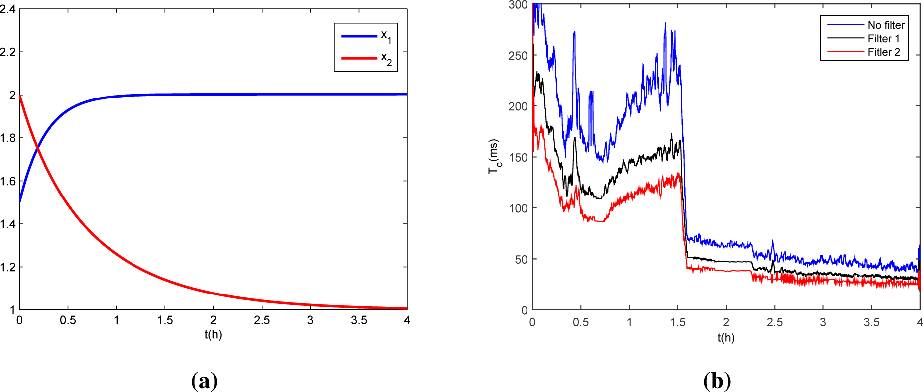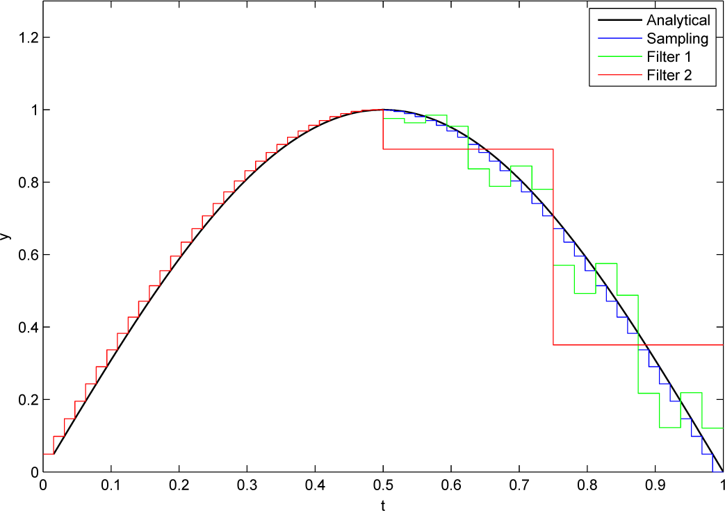Figure 2 shows a sinusoid, y = sin(πt), t ∈ [0, 1], with resolution m = 64 passing though two filters (Filter 1: ignoring indices i = 12–15, 48–63; Filter 2: ignoring indices i = 6–7, 12–15, 24–32, 48–63). Clearly, these are both nonlinear filters, which can provide a good approximation to the original signal for t ∈ [0, 1/2] with a coarse reconstruction for t ∈ [1/2, 1].

As advocated in [34], an effective method to reduce the computational complexity of MPC is to decrease the number of decision variables by providing a fine description of the state and control trajectories in the near future, with a coarser description in the far future. This allows for fine tuning of the decision variable in the near future, with a coarser tuning in the distant future. The intuitive motivation for this is that as only the first step in MPC is ever implemented and due to model inaccuracies (which are especially prevalent in chemical processes), the near future is more important that the distant future. Furthermore, as chemical processes often exhibit dynamics on multiple time-scales (due to, for example, different physical and chemical phenomena and multiple phases), this approach can provide an approach to effectively cover both fast (through a fine description of the near future) and slow (through a long prediction horizon, albeit with a coarser description) dynamics. Thus, this approach can achieve a balance between low computational complexity and high levels of performance. This can also be approved by the simulation result of [35], which gives this kind of time partition scheme through an adaptive online time partition method.

This method is somewhat similar to the move-blocking approach, although the mechanism of its implementation is different. Furthermore, the proposed approach is more flexible than move blocking, as it allows for the frequency content of the flat output trajectory to be manipulated at any point in the prediction horizon, not just at the end of the prediction horizon. Although, in the current paper, we restrict ourselves to this case, as it provides an effective method of decreasing computational time without sacrificing performance. The flat output is ‘blocked’ in the far future, while the stage cost function is not blocked. This approach allows for a significant reduction in the number of decision variables. For example, by implementing Filter 2, the number of decision variables is reduced from 64 to 34. In this way, the frequency content of the flat output trajectory distribution can be viewed as an additional tuning parameter, which the designer can choose based on the process dynamics and required computational and control performance. A potential disadvantage of this approach is a potential reduction of the stability margin, as the resulting solution is suboptimal. Thus, the reduction of Haar wavelet coefficients should be chosen as a balance between the computation cost and system robustness. It should be noted that proving stability when move-blocking is used can be quite difficult, as well. However, for a multiple time scale dynamical system, this is not an issue, because the controller only needs to capture the slow dynamics, not the precise prediction for the fast dynamics, in the far future.

4. Case Study

4.1. A Flat Chemical Reactor Model

The CSTR depicted in Figure 3 is a simplified model of the cyclopentenol synthesis process from [9], with the assumption of constant temperature and volume. The CSTR is fed by a liquid flow containing the reactant A with constant concentration, C_in. There are three reactions occurring inside the reactor, and this reaction scheme is shown in Figure 3 with the desired product being component B, with C and D representing by-products. The material balance equations are given below.

$$\begin{array}{l}{\dot{x}}_1=-k_1{x}_1-k_3{x}_1^2+u\left(C_{in}-x_1\right)\\ {\dot{x}}_2=k_1{x}_1-k_2{x}_2-u{x}_2\end{array}$$

(17)

where x₁(t), x₂(t) are the concentrations of A and B and the manipulated variable, u, is the inlet flow rate. The model parameters and operating point are summarized in

Table 1. System parameters.

Parameter	Description	Unit	Value
Cin	Inlet concentration of A	kg mol/m3	4.9
x1(0)	Initial concentration of A	kg mol/m3	1.5
x2(0)	Initial concentration of B	kg mol/m3	2
$x_1^{\ast }$	Nominal concentration of A	kg mol/m3	2
$x_2^{\ast }$	Nominal concentration of B	kg mol/m3	1
u∗	Nominal flow rate	kg mol/h	1.1
k1	Reaction 1 rate constant	h−1	0.6
k2	Reaction 2 rate constant	h−1	0.1
k3	Reaction 3 rate constant	h−1	0.5

. It can be shown that the CSTR model Equation (17) is differentially flat with the flat output z as defined below [36]:

$$z=\frac{C_{in}-x_1}{x_2}$$

(18)

The system is locally equivalent to a second order integrator as long as following condition is satisfied:

$$\frac{\partial z}{\partial x_1}\left[-2k_1{x}_1-3k_3{x}_1^2+C_{in}\left(k_1+2k_3{x}_1\right)\right]-k_1{C}_{in}\frac{\partial z}{\partial x_2}\ne 0$$

From Equation (18), it can be seen that the flat output has a physical meaning and may be interpreted as a ratio of concentrations. The characteristic of flat outputs for more general nonlinear systems can be found in [8]. Using the model Equation (17) and Equation (18) and its derivatives, we obtain the L-B isomorphic maps between the state/input and the flat output as follows.

$$\begin{array}{l}{x}_1={\varphi }_1(z,\dot{z})=(-b+\sqrt{\mathrm{\Delta }})/2k_3\\ x_2={\varphi }_2(z,\dot{z})=\left(C_{in}-{\varphi }_1\right)/z\\ u={\varphi }_3(z,\dot{z},\ddot{z})=\left(\gamma +k_1{\varphi }_1+k_3{\varphi }_1^2\right)/z{\varphi }_2\end{array}$$

(19)

where $b(z,\dot{z})=k_1-k_2-k_{1}z+\dot{z}/z$, $c(z,\dot{z})=\left(k_2-\dot{z}/z\right)C_{in}$, $\mathrm{\Delta }(z,\dot{z})=b^2-4k_{3}c$, $\gamma (z,\dot{z},\ddot{z})=-\left(\dot{b}{\varphi }_1+\dot{c}\right)/\left(2a{\varphi }_1+b\right)$.

4.2. Simulation Results

Combining Equations (15)–(19), the proposed Haar wavelet-based MPC (HMPC) algorithm was implemented in MATLAB. The simulation result is compared to the standard NMPC approach and the flatness-based MPC using polynomial basis functions (PMPC) presented in [12].

For illustration, in the first series of simulations, no input or state constraints were implemented, and the objective function for all cases was chosen as:

$$J(x,u)={\displaystyle \sum _{i=1}^N\left[0.2{\left(x(i)-x^{\ast }\right)}^T\left(x(i)-x^{\ast }\right)+{\left(u(i)-u^{\ast }\right)}^2\right]}$$

The control objective is to regulate the system to the nominal concentrations given in Table 1. All cases were carried out by MATLAB R2014a on a desktop PC (Windows 7 64-bit OS with an Intel i5-3470 3.2 GHz processor). The optimization problem is solved using an active-set method with a warm start in all cases.

As is shown in

Table 2. Average computation time cost of the controller without the input constraint. HMPC, Haar wavelet-based MPC; PMPC, Polynomial basis MPC; NMPC, nonlinear MPC.

Resolution	HMPC (ms)	PMPC (ms)	NMPC (ms)
m = 4	4.7	6.2	9
m = 8	5.7	9.6	16
m = 16	7.6	22	40
m = 32	20	80	160

, the proposed HMPC algorithm significantly reduces the computational load as compared to the other two methods. In particular, it should be noted that the proposed HMPC approach scales better with increasing prediction horizon, as compared to the other approaches, with the differences in computation time increasing with the optimization horizon of the control (and, therefore, the number of decision variables). There is an acceptable steady-state error in the proposed approach (0.002 in the states and 0.004 in the input at steady state) in the HMPC approach. This steady-state error may be due to the truncation of the infinite Haar wavelet series. This could be counteracted by optimizing Δu, rather than u, thus forcing integral action into the controller as is common in existing MPC formulations. Figure 4 shows the closed loop state response and the corresponding flat output trajectory generated by the HMPC algorithm when the resolution is chosen as m = 16. As the states reach the steady state, the flat output z converges to a constant and its derivative ż tends to zero. The running costs (measured in terms of the cost function for the actual state and input trajectories) of the simulations in Figure 4 are 19.64 for the NMPC approach and 19.65 for both the PMPC and HMPC approaches, thus demonstrating that the proposed HMPC approach achieves a high level of performance and one very similar to that of the other approaches based on the parameterization of the flat output trajectory.

A second simulation was performed with set-point $\left(x_1^{\ast },x_2^{\ast }\right)=(6,3)$, u^* = 1 and with input constraint 0.95 ⩽ u ⩽ 1.05, that is, restraining the flow rate to be within ±5% of the nominal value. Figure 5 shows the state and input trajectories for this case. It is seen that the proposed HMPC algorithm is effective at regulating the system whilst respecting the constraint.

As expected, when the input constraint is put into the MPC algorithm, the computation time increases for higher resolution. As seen in Figure 6b, when m = 64, the average computation time is 200 ms during the transition period, while it reduces to 70 ms during the steady state, which is much larger than that of m = 32 in Table 2. By applying the reduction in the wavelet coefficients technique presented in Section 3.3, the computation time is almost halved as compared to the base HMPC case without any filter applied to the Haar wavelet series. At the same time, from the state trajectory in Figure 6a, it is clear that there is no obvious loss in the control performance by comparing it to the case of m = 16 in Figure 4. Comparing the approaches in Figure 6a,b, the achieved value of the cost function was 77.6 for all three cases (no filter, Filter 1 and Filter 2), thus further demonstrating that shaping the resolution of the Haar wavelet series can effectively decrease the computational time without affecting control performance.

5. Conclusions

A novel and computationally efficient algorithm for NMPC of differentially flat systems has been developed, which is based on a parameterization of the flat output and its derivatives by a finite Haar wavelet series. The proposed approach allows for the dynamic programming problem to be reduced to a finite dimensional static optimization problem, which admits a numerically-efficient solution. This is further facilitated by the nice mathematical properties of Haar wavelets, which allow for efficient numerical integration to reduce the computational burden, as demonstrated in the case study. A key advantage of the proposed approach is the ability to use the integral operation matrix to efficiently integrate the Haar wavelet series representing the highest order derivative of the flat output. In particular, the proposed approach was observed to scale better with the number of decision variables (i.e., optimization horizon) as compared to other methods.

Additionally, the use of Haar wavelets allows for the resolution and frequency content of the flat output trajectory to be shaped by the designer. This allows for a reduction of the number of decision variables by reducing the resolution of the Haar series in the far future, whilst retaining high resolution in the near future. The approach to using a prediction/control horizon with non-uniform resolution may be especially useful for processes that exhibit dynamics on multiple time scales, as it allows for long optimization horizons to capture slow dynamics and high resolution in the near future to capture fast dynamics. Unlike approaches based on singular perturbations, this approach does not require a large separation of time-scales and, thus, may be used for systems with large ranges of dynamics, although without a clear separation of the fast and slow modes.

In the proposed approach, there is a trade-off between computational effort and the accuracy of the calculated optimal control sequence (as determined by the number of Haar wavelet coefficients used). An interesting area of further research may be to study how to balance between the computational cost and system performance. A possible extension of the proposed approach is distributed NMPC for flat systems, in which case, the interactions between subsystems may be represented in terms of the flat outputs. Each subsystem exchanges the flat output trajectories and performs distributed optimization through agent negotiation or a dissipativity condition. Alternatively, the approach could be extended to certain classes of non-flat systems, such as Liouvillian systems, which may be viewed as systems containing a flat subsystem.

References

1. Qin, S.; Badgwell, T. A. Survey of Industrial Model Predictive Control Technology. Control Eng. Pract 2003, 11, 733–764. [Google Scholar]
2. Henson, M. Nonlinear model predictive control: Current status and future directions. Comput. Chem. Eng. 1998, 23, 187–202. [Google Scholar]
3. Mayne, D.; Rawlings, J.B.; Rao, C.V.; Scokaert, P.O.M. Constrained Predictive Control: Stability and Optimality. Automatica 2000, 36, 789–814. [Google Scholar]
4. Diehl, M.; Bock, H.G.; Schlöder, J.P.; Findeisen, R.; Nagy, Z.; Allgöwer, F. Real-time optimization and nonlinear model predictive control of processes governed by differential-algebraic equations. J. Process Control 2002, 12, 577–585. [Google Scholar]
5. Albuquerque, J.; Gopal, V.; Staus, G.; Biegler, L.T.; Ydstie, B.E. Interior point SQP strategies for large-scale, structured process optimization problems. Comput. Chem. Eng. 1999, 23, 543–554. [Google Scholar]
6. Bartusiak, R.D. Assessment and Future Directions of NMPC; Springer: Berlin, Germany, 2007; Chapter NLMP; pp. 367–381. [Google Scholar]
7. Yang, X.; Biegler, L.T. Advanced-multi-step nonlinear model predictive control. J. Process Control 2013, 23, 1116–1128. [Google Scholar]
8. Lévine, J. Analysis and Control of Nonlinear Systems: A Flatness-based Approach; Springer-Verlag: Berlin/Heidelberg, Germany, 2009. [Google Scholar]
9. Rothfuss, R.; Rudolph, J.; Zeitz, M. Flatness Based Control of a Nonlinear Chemical Reactor Model. Automatica 1996, 32, 1433–1439. [Google Scholar]
10. Murray, R.M.; Rathinam, M.; Sluis, W. Differential Flatness of Mechanical Control Systems: A Catalog of Prototype Systems, Proceedings of the ASME International Mechanical Engineering Congress and Expo, San Francisco, CA, USA, 12–17 November 1995.
11. Martin, P.; Devasia, S.; Paden, B. A different look at output tracking: Control of a vtol aircraft. Automatica 1996, 32, 101–107. [Google Scholar]
12. Mahdevan, R.; Agrawal, S.; Doyle, F., III. Differential flatness based nonlinear predictive control of fed-batch bioreactors. Control Eng. Pract 2001, 9, 889–899. [Google Scholar]
13. Flores, M.E.; Milam, M.B. Trajectory Generation for Differentially Flat Systems via NURBS Basis functions with Obstacle Avoidance, Proceedings of the American Control Conference, Minneapolis, MN, USA, 14–16 June 2006.
14. Suryawan, F.; de Doná, J.; Seron, M. Minimum-time trajectory generation for constrained linear systems using flatness and B-splines. Int. J. Control. 2011, 84, 1565–1585. [Google Scholar]
15. Suryawan, F.; de Doná, J.; Seron, M. Splines and polynomial tools for flatness-based constrained motion planning. Int. J. Syst. Sci. 2012, 43, 1396–1411. [Google Scholar]
16. De Doná, J.; Suryawan, F.; Seron, M.; Lévine, J. A flatness-based iterative method for reference trajectory generation in constrained NMPC. In Nonlinear Model Predictive Control; Springer: Berlin, Germany, 2009; pp. 325–333. [Google Scholar]
17. Karimi, H.; Lohmann, B.; Jabedar Maralani, P.; Moshiri, B. A computational method for solving optimal control and parameter estimation of linear systems using Haar wavelets. Int. J. Comput. Math. 2004, 81, 1121–1132. [Google Scholar]
18. Karimi, H.; Moshiri, B.; Lohmann, B.; Jabehdar Maralani, P. Haar Wavelet-Based Approach for Optimal Control of Second-Order Linear Systems in Time Domain. J. Dyn. Control Syst. 2005, 11, 237–252. [Google Scholar]
19. Hsiao, C.; Wang, W. Optimal control of linear time-varying systems via Haar wavelets. J. Optim. Theor. Appl. 1999, 103, 641–655. [Google Scholar]
20. Karimi, H.; Jabedar Maralani, P.; Moshiri, B.; Lohmann, B. Numerically efficient approximations to the optimal control of linear singularly perturbed systems based on Haar wavelets. Int. J. Comput. Math. 2005, 82, 495–507. [Google Scholar]
21. Hsiao, C. Haar wavelet direct method for solving variational problems. Math. Comput. Simul. 2004, 64, 569–585. [Google Scholar]
22. Chen, C.; Hsiao, C. Haar wavelet method for solving lumped- and distributed-parameter systems. IEE Proc. Control Theor. Appl. D 1997, 144, 87–94. [Google Scholar]
23. Fliess, M.; Lévine, J.; Martin, P.; Rouchon, P. On differentially flat nonlinear systems, Proceedings of the IFAC-Symposium, Bordeaux, France, 24–26 June 1992; pp. 408–412.
24. Fliess, M.; Lèvine, J.; Martin, P.; Rouchon, P. Flatness and defect of nonlinear systems: Introductory theory and examples. Int. J. Control. 1995, 61, 1327–1361. [Google Scholar]
25. Lévine, J. On necessary and sufficient conditions for differential flatness. Appl. Algebra Eng. Commun. Comput. 2011, 22, 47–90. [Google Scholar]
26. Martin, P.; Rouchon, P.; Murray, R.M. Flat Systems, Equivalence and Trajectory Generation; Technical Report; California Institute of Technology: Pasadena, CA, USA, 2003. [Google Scholar]
27. Wu, J.L.; Chen, C.H.; Chen, C.F. Numerical inversion of Laplace transform using Haar wavelet operational matrices. IEEE Trans. Circuits Syst. I: Fund. Theor. Appl. 2001, 48, 120–122. [Google Scholar]
28. Wu, J.L. A wavelet operational method for solving fractional partial differential equations numerically. Appl. Math. Comput. 2009, 214, 31–40. [Google Scholar]
29. Chen, H.; Allgöwer, F. A quasi-infinite horizon nonlinear model predictive control scheme with guaranteed stability. Automatica 1998, 34, 1205–1217. [Google Scholar]
30. Yu, S.; Reble, M.; Chen, H.; Allgöwer, F. Inherent robustness properties of quasi-infinite horizon nonlinear model predictive control. Automatica 2014, 50, 2269–2280. [Google Scholar]
31. Liu, J.; Muñoz de la Peña, D.; Ohran, B.J.; Christofides, P.D.; Davis, J.F. A two-tier architecture for networked process control. Chem. Eng. Sci. 2008, 63, 5394–5409. [Google Scholar]
32. Liu, J.; Muñoz de la Peña, D.; Christofides, P. Distributed Model Predictive Control of Nonlinear Process Systems. Am. Inst. Chem. Eng. J 2009, 55, 1171–1184. [Google Scholar]
33. Christofides, P.D.; de la Peña, D.M.; Liu, J. Networked and Distributed Predictive Control: Methods and Nonlinear Process Network Applications; Springer: London, UK, 2011. [Google Scholar]
34. Tippett, M.J.; Tan, C.K.; Bao, J. Non-Constant Prediction-Step MPC for Processes with Multi-Scale Dynamics, Proceedings of the 19th IFAC World Congress, Cape Town, South Africa, 24–29 August 2014.
35. Pannocchia, G.; Rawlings, J.B.; Mayne, D.Q.; Mancuso, G. Whither discrete time model predictive control? IEEE Trans. Autom. Control. 2014, 60, 246–252. [Google Scholar]
36. Sira-Ramirez, H.; Agrawal, S.K. Differentially Flat Systems; Marcel Dekker: New York, NY, USA, 2004; Volume 17. [Google Scholar]
Figure 1. Representation of the flatness property (adapted from [8]).
Processes 03 00161f1
Figure 2. Signal representation with different wavelet coefficient selection.
Processes 03 00161f2
Figure 3. CSTRin the case study.
Processes 03 00161f3
Figure 4. Simulation result with resolution m = 16. (a) Closed loop state trajectory; (b) flat output trajectory.
Processes 03 00161f4
Figure 5. Simulation result under the input constraint with m = 16. (a) State trajectory; (b) input trajectory.
Processes 03 00161f5
Figure 6. MPC with different filters (resolution m = 64). (a) State trajectory by Filter 2; (b) computational time cost.
Processes 03 00161f6