
Forecasting Gas Well Classification Based on a Two-Dimensional Convolutional Neural Network Deep Learning Model
1
State Key Laboratory of Shale Oil and Gas Enrichment Mechanisms and Effective Development, Beijing 100083, China
2
Exploration and Production Research Institute, Sinopec, Beijing 102206, China
3
School of Science, Southwest Petroleum University, Chengdu 610500, China
4
School of Computer Science, Southwest Petroleum University, Chengdu 610500, China
*
Author to whom correspondence should be addressed.
Processes 2024, 12(5), 878; https://doi.org/10.3390/pr12050878
Submission received: 13 March 2024
/
Revised: 12 April 2024
/
Accepted: 17 April 2024
/
Published: 26 April 2024
(This article belongs to the Special Issue Data-Based Prediction Models in Energy Systems: From Principles to Applications)
Abstract
:In response to the limitations of existing evaluation methods for gas well types in tight sandstone gas reservoirs, characterized by low indicator dimensions and a reliance on traditional methods with low prediction accuracy, therefore, a novel approach based on a two-dimensional convolutional neural network (2D-CNN) is proposed for predicting gas well types. First, gas well features are hierarchically selected using variance filtering, correlation coefficients, and the XGBoost algorithm. Then, gas well types are determined via spectral clustering, with each gas well labeled accordingly. Finally, the selected features are inputted, and classification labels are outputted into the 2D-CNN, where convolutional layers extract features of gas well indicators, and the pooling layer, which, trained by the backpropagation of CNN, performs secondary dimensionality reduction. A 2D-CNN gas well classification prediction model is constructed, and the softmax function is employed to determine well classifications. This methodology is applied to a specific tight gas reservoir. The study findings indicate the following: (1) Via two rounds of feature selection using the new algorithm, the number of gas well indicator dimensions is reduced from 29 to 15, thereby reducing the computational complexity of the model. (2) Gas wells are categorized into high, medium, and low types, addressing a deep learning multi-class prediction problem. (3) The new method achieves an accuracy of 0.99 and a loss value of 0.03, outperforming BP neural networks, XGBoost, LightGBM, long short-term memory networks (LSTMs), and one-dimensional convolutional neural networks (1D-CNNs). Overall, this innovative approach demonstrates superior efficacy in predicting gas well types, which is particularly valuable for tight sandstone gas reservoirs.
1. Introduction
The global demand for unconventional resources is rising, driven by the development of oil drilling and production technology. On one hand, with the development of technology, it has become feasible in theory and practice to excavate the hydrocarbons stored in some unconventional resources (such as shale/tight reservoirs) [1]. On the other hand, conventional natural gas reserves have reduced while the global demand for energy continues to increase, emphasizing the need to explore unconventional gas sources [2].
Tight gas sand is one of the most common unconventional natural gas resources in the world, but its low productivity and low permeability increase the difficulty of oil extraction [3]. The standard industry definition of tight gas is a reservoir system with low permeability (usually less than 0.1 mD) and low porosity (usually less than 10%), which usually occurs in sandstone formations, shale formations, and coal seams [4]. In addition, the definition introduces the importance of increasing reservoir production via hydraulic fracturing in modern tight gas.
Tight sandstone gas reservoirs have low porosity, low permeability, strong heterogeneity, poor physical properties, and poor connectivity. During exploitation, the formation pressure decreases quickly, resulting in low production and thus low recovery. Even in the same study area, different gas wells have significant reservoir differences and are exploited in different ways, so it is necessary to classify gas wells in this study area with relatively high accuracy.
With the continuous development of artificial intelligence technology, the advantages of machine learning and deep learning algorithms to improve business decision-making and operational efficiency have always attracted attention within the industry. Machine learning models are trained to predict or classify problems. Deep learning belongs to a branch of machine learning, which is a learning method that uses a deeper network structure to extract more feature information to achieve prediction or classification. The existing traditional machine learning classification methods mainly include K-nearest neighbors, logistic regression, and Fisher discriminant, but the classification effect is good in the case of low-dimensional data, and the effect of solving high-dimensional problems is poor. Therefore, the current mainstream high-dimensional data classification methods are mainly deep learning algorithms, including the single model of 1D-CNN, 2D-CNN, LSTM, or the hybrid model of CNN-LSTM.
The problem of gas well class prediction in tight sandstone gas reservoirs can be mainly divided into two categories, namely binary class prediction and multi-class prediction problems. The problem of class prediction has also been solved in different areas, such as medicine, finance, and sentiment analysis. In addition, there have been studies using 2D-CNN models for binary class prediction in the financial and medical industries. For example, Weina Qin proposed a financial risk early warning method based on a convolutional neural network and compared it with three other models, finding that the prediction accuracy of the new model was 97.1%, which was significantly higher than that of other models [5] li Ghulam et al. proposed a new method based on deep learning to improve the prediction of the dichotomous classification of anticancer peptides. They extracted important features via the deviation between the dipeptide and the expected average (DDE). Meanwhile, they utilize the 2D-CNN model to train and predict the data set. The accuracy of the model on the test set is 75%. The experimental results show that this method achieves the best performance and can predict ACPs more accurately than the existing methods in all the articles [6]. In addition, speech emotion recognition has also employed multi-class prediction. For example, Jianfeng Zhao et al. used the 1D-CNN-LSTM network and 2D-CNN-LSTM network to learn deep emotion features to recognize speech emotion. Their performance is superior to the traditional methods of deep belief network (DBN) and CNN in the selected database. The 2D-CNN-LSTM network has achieved 95.33% and 95.89% recognition accuracy based on speaker experiment and independent speaker experiment, respectively; which are excellent performances in speech emotion recognition [7].
Because little research has been conducted for the identification of gas well types in tight sandstone gas reservoirs, in this paper, research has been conducted on the identification of oil and gas reservoirs to the drilling safety risks. As for the binary prediction model, Shaowei Pan et al. synthesised the features and advantages of CNN and LSTM, and built a combined model containing CNN and LSTM to more accurately mine the internal correlations in the oil well production data, thus improving the prediction accuracy [8]. In order to further improve the efficiency of the model and reduce the dependence on parameters, some drilling parameters closely related to overflow were selected. The experiments show that the network structure using CNN-LSTM is superior to the single CNN and the single LSTM structure, and the prediction accuracy can reach 89.55% [9]. For the multi-class prediction problem, HU Wanjun et al. used the method of combining the convolution neural network and BP neural network to deeply and effectively identify the safety risk characteristics in gas drilling, and they obtained that the identification accuracy of various potential risks in gas drilling is about 90% [10]. In addition, in order to improve the identification accuracy of high-quality reservoirs in the reservoir, Linqi Zhu et al. proposed a method combining the over-sampling method based on logging data and the random forest algorithm, which remarkably improved the accuracy of reservoir identification from 44% to 78% compared with other machine learning algorithms [11]. But, the prediction accuracy of oil and gas reservoir identification and drilling safety risk identification is still lower than 90%. Since the accuracy of the 2D-CNN-LSTM model in multi-class prediction of speech emotion recognition has reached more than 95%, this model can also be applied to multi-class prediction of gas well types in tight sandstone.
This article used a new method based on a two-dimensional convolutional neural network (2D-CNN) in deep learning. Utilizing the significant characteristics of the gas well excavated by the convolution layer, the calculation depth of the network is surged by increasing the convolution operation, thus improving the prediction accuracy of the model. So, in this paper, the 2D-CNN model is first applied to the classified prediction of tight sandstone gas wells, realizing the identification of gas well types and then effectively evaluating the field operation of the gas field.
2. Materials and Methods
2.1. XGBoost Algorithm
XGBoost version 1.4.2 is an effective decision tree algorithm [12]. As a common machine learning algorithm, a decision tree is often used for classification problems. Due to its low computational complexity, easy interpretation of output results, insensitivity to missing intermediate values, and ability to deal with irrelevant feature variables, it has been widely used in data analysis and data mining [13]. However, the potential of decision tree models is limited by problems such as poor stability, sensitivity to data distribution, propensity to fit, and unreliable generalization performance. With the development of artificial intelligence technology, the XGBoost algorithm has shown good performance on classification problems [14]. It integrates multiple weak learners via combinatorial learning to build a strong learner to eliminate these limitations and improve its performance.
Due to its high performance in dealing with classification problems, it has been widely used in the field of data mining and intelligent prediction. The objective function of the XGBoost model includes a loss function and a regularization term. The regularization term controls the complexity of the tree model to achieve optimization and prevent the overfitting problem, which also provides a fast and reliable model for many engineering simulations. The formula for data prediction using the XGBoost model is as follows:
where —real value, —the prediction at the t-th round, —loss function, —a term denoting the structure of the decision tree, and —regularization term given by the following formula:
where and are penalty coefficients, —number of leaves, and —weight of leaves.
2.2. Spectral Clustering
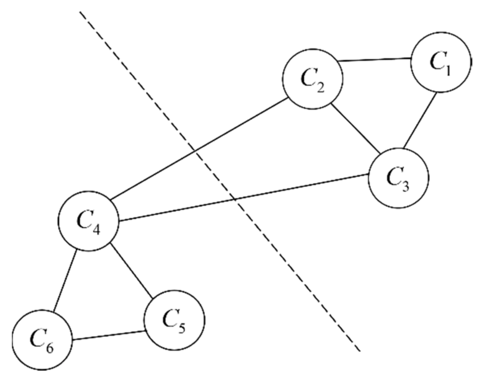
Compared with the traditional K-means clustering, spectral clustering (SC) [15] is more adaptable to data, which has a more ideal clustering effect, and it is easy to implement, so it has been widely used. SC is based on graph theory, and its core idea is to treat each sample in the data set as a vertex in the space, and these vertices can be connected by edges. The edge weight is given by quantifying the similarity between variables. The higher the similarity, the greater the weight and the closer the distance between the variables. For a graph , it is described by the set of points and the set of edges, namely m, as shown in Figure 1.
The goal of SC is to maximize the sum of weights within subgraphs and minimize the sum of weights between subgraphs via graph cutting.
In order to quantify the similarity of gas well development indicators, vectors and are set, and the Pearson correlation coefficient between them is
where is the average value of vector , and is the average of vector .
Pearson’s correlation coefficient of gas well development index is calculated. Then, the spatial distance between gas layers is calculated to form the distance matrix , and the two matrices are linearly weighted as the similarity measurement matrix .
where is a Pearson matrix, and are the weights, and . Different clustering results can be obtained by adjusting the weights.
2.3. Convolutional Neural Network
The convolutional neural network (CNN) [16] is a kind of feedforward neural network, which has been successfully applied in the classification task with the time series data and the image data by its powerful feature extraction and recognition ability. Its basic structure consists of the input layer, convolution layer, pooling layer, fully connected layer (FC), and output layer. The convolution layer and pooling layer are specially designed data processing layers, which are used to filter input data and extract useful information. Pooling layer screens features, extracts the most representative features, reduces the dimensions of the features, and makes the features robust to noises [17]. The fully connected layer summarizes the learned features and maps them into two-dimensional feature output.
In convolutional neural networks, the biggest advantage that distinguishes them from other neural networks are local receptive fields and weight sharing. Via these two methods, the invariance of the network to the displacement, scaling, and distortion of the input are realized. Local receptive fields can extract local and primary features. Weight sharing can make the network have fewer free parameters, reduce the complexity of the network model, reduce the overfitting, and improve the generalization ability. Moreover, the BN layer standardizes the activation of each batch of convolutional layers and improves the performance and stability of deep networks. The transformation applied by batch normalization keeps the mean activation close to 0 and the activation standard deviation close to 1 [7]. The RELU function is used as the activation function to define the output of the BN layer. The nonlinear features can be obtained via the activation function to enhance the feature expression ability of the model. Therefore, the convergence process of convolutional neural networks can be accelerated, and the recognition accuracy can be improved.
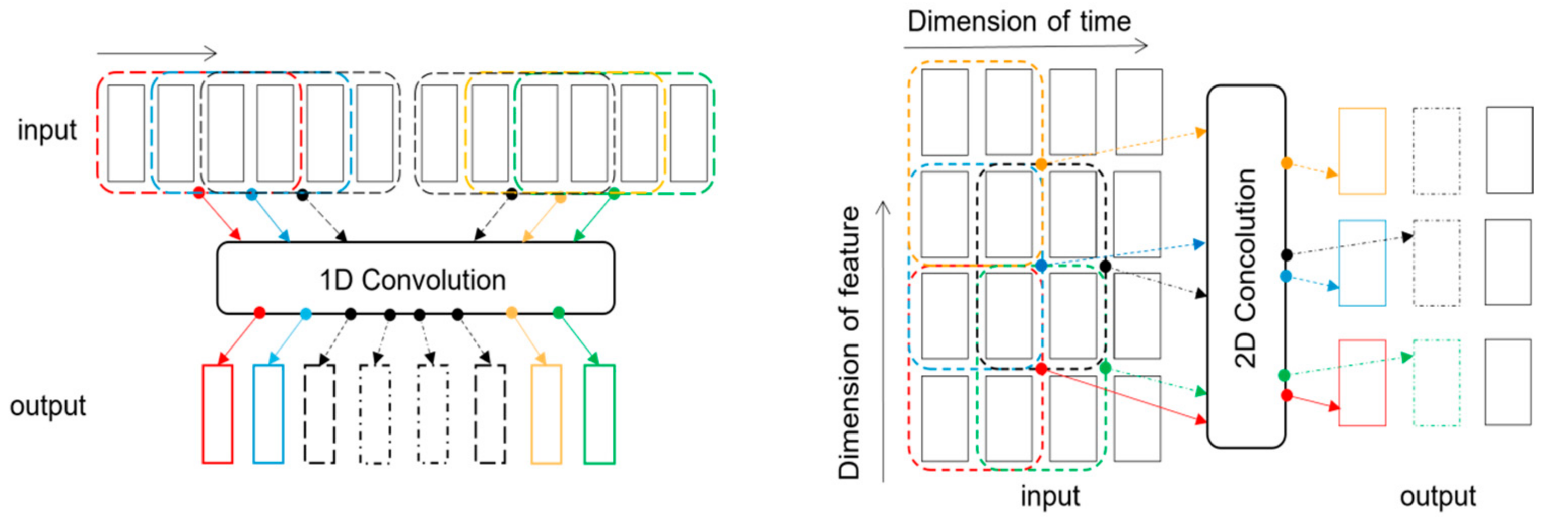
There are two main forms of CNN models, which can be divided into a one-dimensional convolutional neural network (1D-CNN) and a two-dimensional convolutional neural network (2D-CNN) according to the different moving directions of the convolutional kernel in CNN. Compared with the unidirectional movement mode of the former convolution kernel, the bidirectional movement mode of the 2D-CNN convolution kernel can better extract the features so as to improve the prediction accuracy of the classification. Therefore, the input form of 1D-CNN is improved; that is, the time series data in the one-dimensional form are transformed into the image data in the two-dimensional form, and the 2D-CNN model is obtained. Due to the different dimensions of input variables, the corresponding operation modes of the convolution layer and pooling layer are also different. The following part describes the convolution operation and pooling operation of the convolution layer and pooling layer from 1D-CNN and 2D-CNN, respectively.
2.3.1. Convolution Layer
One-dimensional convolutional neural networks can be well applied to process the basic features of specific data of different time periods and sequence types, so they have great application space in the field of natural language processing, such as speech recognition and speech synthesis. The connection mode between neurons in the 1D-CNN model is a local connection, which changes the full connection mode of the traditional BP neural network into the local connection mode of the convolutional neural network and has the feature of shared weight. The convolution kernel is introduced into the one-dimensional convolutional neural network, and the matrix features are extracted via the convolution operation of the convolution kernel and input variables. The output value is composed of multiple feature surfaces, each value of the feature face represents a neuron, and the value of each neuron in the feature surface is calculated by the convolution kernel.
However, the two-dimensional convolutional neural network is considered to be the most widely used and technologically mature convolutional neural network at present, mainly applied in computer vision and image processing. Different from the horizontal sliding mode of the convolution kernel in the 1D-CNN model, the 2D-CNN model is divided into two dimensions for convolution operation. The movement direction of the convolution kernel is to extract the horizontal gas well development features first and then extract the vertical time features. This bidirectional movement method can more completely extract the development features that affect the prediction of gas well types. Thus, the classification accuracy of gas well type prediction can be improved. The convolution operations of the convolution layer of the 1D-CNN and 2D-CNN models are shown in Figure 2.
If the input variable is time series data in one-dimensional form, the data are passed into the convolution layer. It will be convolved with the convolution kernels across the width and height of the input volume. Then, the feature map is produced by calculating the product between the entries of the kernel and the input, and the output of the -th neuron in the convolution layer in 1D-CNN is obtained as follows:
where represents the shared weight of convolution kernel among neurons, denotes the number of convolution kernels, represents the offset of the -th convolution check in the hidden layer, and is the activation function.
If the input variable is two-dimensional image data, it will also be convolved with the convolution kernel in terms of the width and height of the input volume. The difference is that the convolution kernel and input data structure of the 1D-CNN model in Equation (11) need to be improved to transform one-dimensional data into two-dimensional data. Assuming the dimension of the convolution kernel of the 1D-CNN model and the dimension of the convolution kernel of the 2D-CNN model, the formula for calculating the convolution layer of the 2D-CNN model is
where represents the output value of the -th neuron of the -th feature surface, represents the weights corresponding to row and column in the -th convolution kernel, and is the offset value of the -th convolution check in the convolutional layer.
2.3.2. Max-Pooling Layer
In order to extract significant features from the gas well development time series and retain more information, a pooling operation is performed after the convolution layer, which is a process of secondary extraction of data features. The pooling layer is mainly operated by the pooling function, which is a form of downward sampling, also known as the subsampling layer in a neural network. Similarly, the 1D-CNN model is a unidirectional pooling operation while the 2D-CNN model is a bidirectional pooling operation. The gas well development features of the feature dimension are extracted first, and then the time features of the time dimension are extracted. The pooling operation of 1D-CNN and 2D-CNN model pooling is shown in Figure 3.
There are two common pooling operations: mean pooling and maximum pooling. Mean pooling takes the mean value of neurons in the perception domain as the output value, while maximum pooling takes the maximum value of neurons in the perception domain as the output. In practice, the maximum pooling function is generally used to take the maximum value of the feature region as the value of the new abstract region, thus reducing the size of the data space. The number of parameters and the amount of computation will also be reduced, reducing the number and complexity of full connections and avoiding overfitting to a certain extent [18]. The mathematical expression of the maximum pooling function is shown as Equation (7):
where is the output value of the -th neuron on the -th feature surface. is the output value after the pooling of the -th neuron on the -th feature surface. is the width of the pooled window.
3. Results
3.1. Data Source
Based on the previous investigation, the original sample data of a tight sandstone gas reservoir in Sichuan Province were collected, with a total of 29 development indicators, which are mainly divided into the geological factors (14) and engineering factors (15). The geological factors are the internal characteristics of the gas reservoir itself, while the engineering factors are the external characteristics affecting the evaluation of gas well types of tight gas reservoirs. Geological factors affecting the evaluation of gas well types in tight gas reservoirs include uncontrollable factors such as porosity, permeability, initial gas saturation, and reservoir thickness, while engineering factors affecting the evaluation of gas wells include controllable factors such as casing inner diameter, tubing inner diameter, tubing outer diameter, and perforation thickness. Therefore, the prediction accuracy of gas production by adjusting the scope of engineering factors in this article can be improved, and a scientifically reasonable gas well evaluation is conducted. The specific indicators of geological factors and engineering factors effecting the evaluation of gas wells are shown in Table 1.
3.2. Selection of Main Control Factors
In order to improve the classification accuracy of the model and reduce the calculation time of the model, the original sample data should be pre-processed before evaluating the gas well type. The main methods are the variance filtering method, correlation coefficient method, and XGBoost algorithm.
Firstly, the feature with a variance of 0 is eliminated. When the variance of a group of data is 0, it means that there is basically no difference in the value of this group of data, so it is not suitable for data analysis and should be eliminated. According to this principle, among the 15 original sample data, the variance of the development indicators of fracturing and horizontal section length is 0, so these two indicators are eliminated.
Secondly, the Pearson correlation coefficient method is used to eliminate the features with a correlation coefficient greater than 0.8. The correlation coefficient reflects the degree and direction of correlation between the two factors, ranging from −1 to 1. If the absolute correlation coefficient of two features is bigger, the correlation between two features is stronger. The classification effect of the model can be improved by deleting features with high correlation. The correlation coefficient method is used to calculate the correlation coefficient between the two indicators and draw the corresponding thermodynamic diagram of the two indicators (see Figure 4). Since the empirical formulas corresponding to the gas deviation factor, gas volume coefficient, the absolute density of formation water, and rock compressibility coefficient are highly correlated, these four indicators should be eliminated. Finally, seven indicators deleted by the correlation coefficient method are reservoir thickness, reservoir depth, gas deviation factor, gas volume coefficient, the absolute density of formation water, and rock compressibility coefficient.
Finally, the XGBoost algorithm in feature selection is used to calculate the importance of features. The XGBoost model is constructed by taking the characteristics obtained by the variance filtering method and correlation coefficient method as independent variables and the open flow rate as dependent variables to calculate the characteristic importance of gas well development indicators (see Figure 5). We take 0.04 as the critical value of feature importance and retain the indicators whose importance is greater than 0.04.
The final retained gas well development indicators are effective porosity, effective fracture half-length, gas relative density, casing depth, total fracturing sand volume, original formation temperature, initial gas saturation, skin factor, fracturing fluid flowback rate, formation water salinity, permeability, and perforation thickness. At the same time, in combination with the background knowledge of gas reservoir development, considering that the initial formation pressure will affect the evaluation of gas well types, the index of initial formation pressure is retained as the influencing factor of classification evaluation.
3.3. Evaluation of Gas Well Types
Since the spectral clustering algorithm is an unsupervised learning algorithm, 15 gas well development indicators such as initial formation pressure, original formation temperature, effective porosity, and open flow rate are used as the input of the spectral clustering algorithm, and then the clustering results of gas well types are obtained according to the following five steps. In addition, according to the productivity of gas wells, gas wells are divided into three types: inferior wells, medium-productive wells, and high-productive wells. This can be seen in Figure 6.
STEP1: Determine the number of clusters , input the gas well development data of dimension , and construct the similarity matrix .
STEP2: Calculate the degree matrix . The degree matrix is a diagonal matrix, where the diagonal elements are the sum of the elements in the row.
STEP3: Construct the Laplace matrix and standardize it.
STEP4: Take the first three minimum eigenvalues of and the corresponding eigenvector, normalize the eigenvector, and construct a new matrix .
STEP5: K-means clustering is applied to the row vector of matrix , which corresponds to the original data to obtain the partition C1, C2, C3 of three clusters. Then, take the open flow capacity as the x-axis, the flowback rate of fracturing fluid as the y-axis, and the prime stratum temperature as the z-axis to draw a three-dimensional effect map of spectral clustering so as to show the classification effect of inferior wells, medium-productive wells, and high-productive wells, such as Figure 7.
4. Application
4.1. Model Thinking
In the research on prediction of gas well types in tight gas reservoirs, although the basic theory of traditional machine learning algorithm has been relatively perfect and the method is simple and feasible, there are some problems in the prediction of gas well types using multidimensional gas well development data, such as low prediction accuracy, complex basic theoretical formula, and long algorithm running time. As a commonly used model for processing multidimensional data, deep learning can just overcome these shortcomings. It also provides a new idea for gas well type prediction of multidimensional gas well development data. Due to the low computational depth of the 1D-CNN model, the prediction accuracy of the classification model needs to be improved. Therefore, in order to improve the prediction effect of the classification model, the 2D-CNN model is applied to the classification prediction of gas well types so as to realize the productivity evaluation of tight sandstone gas reservoirs.
The construction idea of the prediction model of gas well types based on 2D-CNN is as follows: firstly, the variance filtering method, correlation coefficient method, and XGBoost algorithm are used to select the features of dimension reduction for the original gas well sample data of a tight sandstone gas reservoir, and then the spectral clustering method is used to classify to determine the three types of gas wells, namely the low-quality well, the medium well, and the high-yield well. Then, the new gas well development index after feature selection is used as the input of the 2D-CNN model via the convolution operation of the convolution layer and the secondary dimension reduction operation of the pooling layer. Finally, the predicted gas well types will be output so as to solve the multidimensional prediction problem of gas well types.
4.2. Model Building Steps
In order to solve the problem of multi-class prediction of multidimensional gas well development data, a new gas well type prediction model based on the 2D-CNN depth learning algorithm is proposed. The prediction process of the model is mainly divided into the following three steps: feature selection of original data, classification of gas well types, and building a 2D-CNN model to predict gas well types. The specific structure of the gas well type prediction model is shown in Figure 8.
- Feature selection of original data
By collecting the original sample data of a gas well in the tight gas reservoir, the original gas well development index and gas well type are determined. Firstly, the feature with a variance of 0 is deleted by the variance filtering method. Secondly, the correlation coefficient method is used to delete the features with a strong correlation. Finally, the XGBoost algorithm is used to sort the original gas well development indicators according to their importance, and new development indicators with feature importance greater than 0.04 are retained to reduce the dimensions of the original data once so as to ensure the effectiveness and accuracy of the subsequent modeling process. At the same time, considering that the initial formation pressure will affect the gas production of gas wells in tight sandstone gas reservoirs, the development index of gas wells with initial formation pressure is retained.
- Classification of gas well types
The spectral clustering algorithm is used to classify the original gas well types. First, according to the productivity of gas wells, the number of clusters is determined to be 3 so as to build a similarity matrix. Secondly, the degree matrix is calculated, and then the Laplace matrix is constructed and standardized. Thirdly, the first three minimum eigenvalues and corresponding eigenvectors are taken, the eigenvectors are normalized, and a new matrix is built. Finally, K-means clustering is applied to the row vectors of the new matrix, corresponding to the original data, and the classification results of three gas well types are obtained.
- Building a 2D-CNN model to predict gas well types
The vector of gas well development indicators after feature selection is expanded, and the vector of new development indicators is matrix processed. The convolution kernel is introduced into the 2D-CNN model, and the new development index matrix is used as the input of the 2D-CNN depth learning model. The characteristics of the gas well development index are extracted via the convolution kernel, and then the classified prediction results of the gas well types are finally output via the secondary dimension reduction of the pooling layer and the calculation of the full connecting layer.
5. Discussion
5.1. Evaluation Performance of The Model
In the field of deep learning, the accuracy, precision, recall, and F1 score [19] are used to evaluate the gas well type, which can objectively and scientifically evaluate the overall performance of the 2D-CNN model. Among them, the accuracy rate is the most intuitive evaluation indicator, but it is not suitable for classification problems with unbalanced categories. Its range is [0, 1]. The higher the value, the stronger the model’s ability to distinguish negative samples. The recall rate represents the ability of the classifier to find all positive samples, with the range of [0, 1]. The higher the number, the stronger the model’s ability to recognize positive samples. The F1 score is a comprehensive expression of both. The range is [0, 1]. The higher the value, the more robust the model [20].
where represents the number of positive samples and correct predictions, represents the number of negative samples and correct predictions, represents the number of positive samples and prediction errors, and represents the number of negative samples and prediction errors.
where is the cross-entropy loss function, and is the output value of the fully connected layer. is the real gas well type obtained by spectral clustering, indicating a high-production well, medium-productive well, and inferior well, respectively. is the value after the regression of function.
In addition, in order to prove the effectiveness of the 2D-CNN model classification, the classification performance is also illustrated via the confusion matrix. Among them, the confusion matrix is an error matrix used to indicate whether the test results belong to the real category.
5.2. Parameter Setting and Prediction Process of 2D-CNN Model
The 2D-CNN model adopts the supervised learning training method, and the training process is divided into forward training and reverse training. Firstly, determining the structure of the two-dimensional convolutional neural network, that is, setting the parameters of each layer in the initial network structure, including the size of the convolution kernel, the size of the pooled kernel, step size, activation function, etc. Then, the two-dimensional characteristic matrix after the structure reconstruction is used as the input of the model, and forward training is carried out. The real and predicted gas well types in the training samples of the model are compared using evaluation indicators to obtain the accuracy and the loss value of the model. Finally, backpropagation is carried out, and the weight matrix is updated continuously using the optimization algorithm to obtain optimal accuracy.
The prediction model of gas well type based on 2D-CNN is mainly composed of two layers of convolution, two pools, and two full connecting layers. In front of the first layer of the two-dimensional convolution layer, there is also a full connection layer whose activation function is Relu, which can add nonlinearity to the deep learning network [21]. For the first convolution layer, the number of convolution kernels is 4, the size of convolution kernels is 2 × 2, and the step size is 2 × 2. In order to prevent gradient loss during model training, a batch normalization layer is usually added behind the convolution layer. The maximum pooling layer follows: the size of pooling kernels is 2 × 2, and the step size is 1 × 1. Next is the second convolution layer. The number of convolution kernels is 2, the size of convolution kernels is 4 × 4, and the step size is 2 × 2. For the second pooled layer, the size of the pooled kernel is 1 × 1, and the above filling methods are all full filling (same). To prevent the model from overfitting, a dropout layer is added, and the p value is set to 0.5; 50% of the information is discarded. Finally, two full connection layers are connected to output the classification results of three gas well types.
When the 2D-CNN model is trained, the input variable is a 15-dimensional gas well development index, and the output is a one-dimensional gas well type. Overall, 186 sample data sets are divided into training sets and testing machines according to a ratio of 7:3. In the training process, the number of iterations is set to 100, the size of the training batch to 4, and the learning rate to 0.001. The activation function in the full connection layer uses the Relu function, and the output layer uses the softmax function and cross-entropy loss function. The optimization algorithm is the Adam algorithm. The parameters of the model are continuously adjusted via gradient descent, and finally, the optimal model parameters are obtained. Among them, the parameters for initializing the model, including convolution kernel size, pooling kernel size, step size, activation function, number of convolution layers, and number of features, are set empirically. The specific structures and parameters of the convoluted layer and pooling layer of the 2D-CNN prediction model are shown in Table 2.
The 2D-CNN model is used to predict the types of gas wells. The prediction model is mainly composed of the input layer, convolution layer, pooling layer, and full connecting layer. The prediction process of the model is shown in Figure 9. The specific process of the multidimensional gas well type prediction model based on 2D-CNN is as follows:
- The variance filtering method and the correlation coefficient method are used to select the preliminary features, and then the XGBoost algorithm is used to determine the new gas well development indicators whose feature importance is greater than 0.04. Then, the input data are divided into a training set and a test set, and one_hot code is used to digitize the gas well type of the test set.
- The training set trains the neural network, extracts information via the convolution layer of the 2D-CNN model, learns the characteristics of gas well development, and uses the BPTT algorithm to backpropagate the training error and continuously update the model parameters.
- The Softmax function is used to obtain the classification probability of three types of gas wells. In order to avoid over fitting of the model, the parameters of the model are constantly adjusted through gradient descent to obtain the optimal parameters of the prediction model.
- Judge whether the network epoch reaches the preset 100 times. If yes, run the next step; otherwise repeat step 2.
- The test set verifies the performance of the trained model, calculates the evaluation indexes, and outputs the prediction results of gas well types.
5.3. Predictive Results of Gas Layers Using 2D-CNN Model
The 2D-CNN model is used in this article to predict the type of gas well, and the inputs are the gas well development indicators after feature selection. After the operation of the convolution layer, pooling layer, and full connecting layer in the convolution neural network, the probability of each sample corresponding to the type of gas well is obtained via the softmax function. The category with higher probability is taken as the gas well type, and finally, the prediction result of the multi-category gas well type is output. The loss value and accuracy of the training set and test set are used to measure the effect of multi-class prediction. The change curve of loss value and accuracy of the prediction model is shown in Figure 10.
The 2D-CNN model is used to classify gas well types. When the number of iterations reaches 100, the curve of loss value and accuracy rate tends to be stable, the accuracy rate of test set reaches 0.99, and the loss value is 0.03, which indicates that the 2D-CNN model shows a good prediction effect in the multi-class prediction of gas well types. The confusion matrix corresponding to the sample number of gas well type classification results obtained from the 2D-CNN prediction model is shown in Figure 11.
The average accuracy of the 2D-CNN multi-category prediction model is 0.99, the average recall rate is 0.99, and the average F1 score is 0.99, as can be seen in Table 3. It can be seen that the model has a strong ability to distinguish between negative samples and positive samples, and the model is relatively robust.
5.4. Comparison with Other Classification Prediction Algorithms
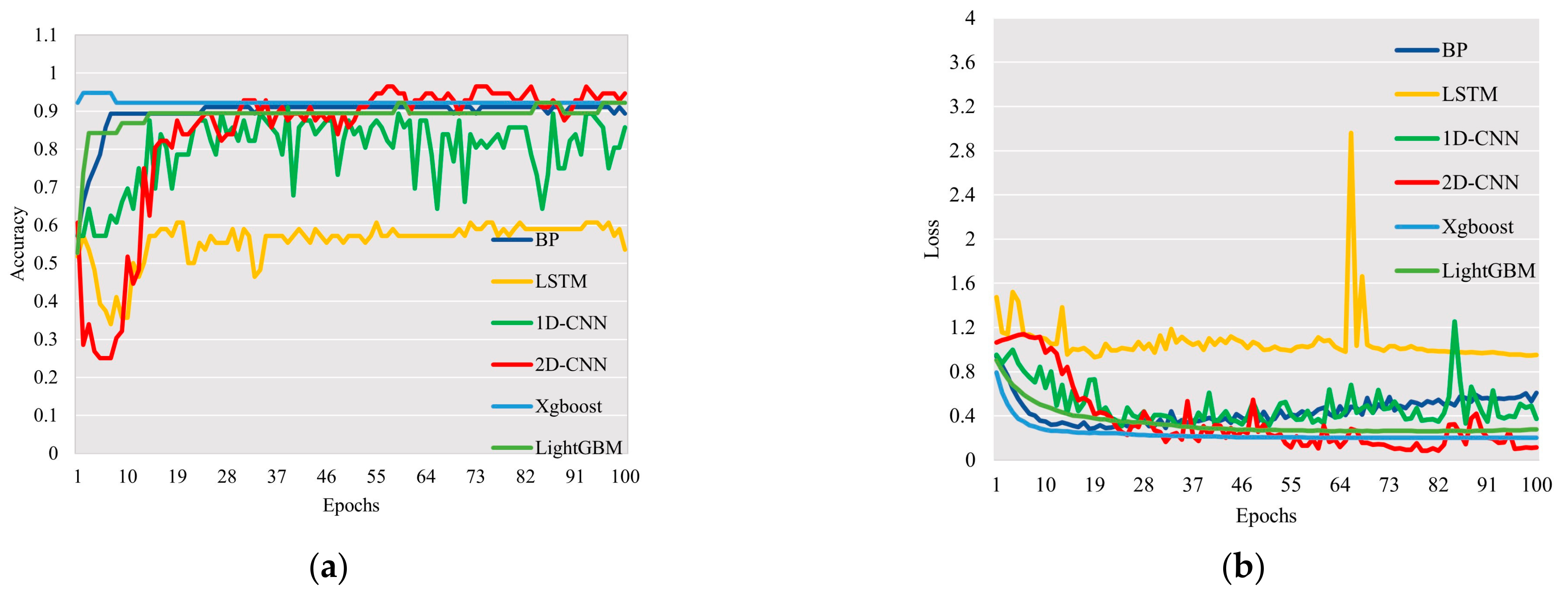
In order to further verify the effectiveness of the multi-class prediction model based on 2D-CNN gas well type, the author compares it with the BP neural network model, XGBoost model, LightGBM (Light Gradient Boosting Machine) model, LSTM model, and 1D-CNN model. The keras module of Python software version 3.7.0 is used to modify the input layer of the model and adjust the parameters of the convolution neural network without changing the basic structure of the model so that it is suitable for the multi-class problem of gas well type prediction. Different models are used to predict the types of gas wells, and the accuracy, loss value, accuracy, recall rate, and F1 value are used as evaluation indicators to measure the prediction effect of the model. As the number of iterations increases, the comparison of accuracy and loss values of different models is shown in Figure 12, and the comparison of evaluation indicators of different models is shown in Table 4.
As the loss value of the 1D-CNN model is significantly lower than that of the BP neural network model and LSTM model and slightly higher than the XGBoost model and LightGBM model, the accuracy of the 2D-CNN model is significantly higher than that of the BP neural network model, XGBoost model, LightGBM model and LSTM model, which indicates that the convolution kernel in convolution neural network can better learn the characteristics of gas well development indicators, extract more significant indicators for prediction, and thus improve the accuracy of gas well type prediction results. According to the experimental results in Table 4, the accuracy rate of the gas well type prediction model built by the author based on the 2D-CNN depth learning method is 0.99, the average accuracy rate is 0.99, the average recall rate is 0.99, and the average F1 value is 0.99, which is better than the prediction effect of the BP neural network model, XGBoost model, LightGBM model, LSTM model, and 1D-CNN model. The minimum accuracy rate on the test set is 0.03.
6. Conclusions
A prediction model based on the 2D-CNN deep learning algorithm is applied in this article, which solves the multi-class problem of gas well type prediction. The prediction results have a strong influence on the evaluation of gas well type. Based on the results of this study, the following conclusions are drawn, and relevant suggestions are provided:
- The spectral clustering algorithm is used to classify various gas well types in tight sandstone gas reservoirs, and three gas well types are obtained. Then, the variance filtering method, correlation coefficient method, and XGBoost algorithm are used to select the characteristics of gas well development indicators and determine new gas well development indicators that affect gas well types. A reasonable selection of development indicators is conducive to improving the multi-class prediction effect of gas well types.
- The double-layer 2D-CNN depth learning method is applied to the multi-class prediction of gas well types. The accuracy of the model is 0.99, and the loss value is 0.03, which is superior to the prediction effect of the BP neural network, XGBoost model, LightGBM model, LSTM model, and 1D-CNN model. Because the 2D-CNN model has a deeper calculation depth, which improves the prediction accuracy of the model, the 2D-CNN model is applicable to the research of gas well type prediction.
- According to the multi-class problem of gas well types, a deep learning model based on 2D-CNN model is proposed. The prediction of gas well types with small sample size has good accuracy and effectiveness, and the accuracy will be significantly improved in the prediction problem with large sample size. Therefore, this method provides a new idea for the prediction research of gas well types with large sample size.
Author Contributions
Conceptualization, C.Z. and Y.J.; methodology, Y.Q.; software, B.W.; validation, W.Z. and S.H.; investigation, C.Z.; resources, Y.J.; data curation, C.Z.; writing—original draft preparation, Y.Q.; writing—review and editing, C.Z. All authors have read and agreed to the published version of the manuscript.
Funding
This research was funded by the Open Fund of State Key Laboratory of Shale Oil and Gas Enrichment Mechanisms and Effective Development.
Data Availability Statement
Data are contained within the article.
Conflicts of Interest
Author Ying Jia was employed by the company Sinopec. The remaining authors declare that the research was conducted in the absence of any commercial or financial relationships that could be construed as a potential conflict of interest. Sinopec had no role in the design of the study; in the collection, analyses, or interpretation of data; in the writing of the manuscript, or in the decision to publish the results.
References
- Kulga, B.; Artun, E.; Ertekin, T. Development of a data-driven forecasting tool for hydraulically fractured, horizontal wells in tight-gas sands. Comput. Geosci. 2017, 103, 99–110. [Google Scholar] [CrossRef]
- Ostojic, J.; Rezaee, R.; Bahrami, H. Production performance of hydraulic fractures in tight gas sands, a numerical simulation approach. J. Pet. Sci. Eng. 2012, 88–89, 75–81. [Google Scholar] [CrossRef]
- Piyush, P.; Kumar, V. Well Testing in Tight Gas Reservoir: Today’s Challenge and Future’s Opportunity. In Proceedings of the the SPE Oil and Gas India Conference and Exhibition, Society of Petroleum Engineers, Mumbai, India, 20–22 January 2010. [Google Scholar] [CrossRef]
- Law, B.; Curtis, J. Introduction to unconventional petroleum systems. AAPG Bull. 2002, 86, 1851–1852. [Google Scholar]
- Qin, W. Research on Financial Risk Forecast Model of Listed Companies Based on Convolutional Neural Network. Sci. Program. 2022, 2022, 3652931. [Google Scholar] [CrossRef]
- Ghulam, A.; Ali, F.; Sikander, R.; Ahmad, A.; Ahmed, A.; Patil, S. ACP-2DCNN: Deep learningbased model for improving prediction of anticancer peptides using two-dimensional convolutional neural network. Chemom. Intel-Ligent Lab. Syst. 2022, 226, 104589. [Google Scholar] [CrossRef]
- Zhao, J.; Mao, X.; Chen, L. Speech emotion recognition using deep 1D & 2D CNN LSTM networks. Biomed. Signal Process. Control 2018, 47, 312–323. [Google Scholar] [CrossRef]
- Pan, S.; Yang, B.; Wang, S.; Guo, Z.; Wang, L.; Liu, J.; Wu, S. Oil well production prediction based on CNN-LSTM model with self-attention mechanism. Energy 2023, 284, 128701. [Google Scholar] [CrossRef]
- Chen, Z.; Yu, W.; Liang, J.-T.; Wang, S.; Liang, H.-C. Application of statistical machine learning clustering algorithms to improve EUR predictions using decline curve analysis in shale-gas reservoirs. J. Pet. Sci. Eng. 2021, 208, 109216. [Google Scholar] [CrossRef]
- Wanjun, H.; Wenhe, X.; Yongjie, L.; Jiang, J.; Gao, L.I.; Yijian, C. An intelligent identification method of safety risk while drilling in gas drilling. Pet. Explor. Dev. 2022, 49, 428–437. [Google Scholar]
- Zhu, L.; Zhou, X.; Zhang, C. Rapid identification of high-quality marine shale gas reservoirs based on the oversampling method and random forest algorithm. Artif. Intell. Geosci. 2021, 2, 76–81. [Google Scholar] [CrossRef]
- Tyagi, P.; Sharma, A.; Semwal, R.; Tiwary, U.S.; Varadwaj, P.K. XGBoost odor prediction model: Finding the structure-odor relationship of odorant molecules using the extreme gradient boosting algorithm. J. Biomol. Struct. Dyn. 2023, 1–12. [Google Scholar] [CrossRef]
- Sun, M.; Yang, J.; Yang, C.; Wang, W.; Wang, X.; Li, H. Research on prediction of PPV in open-pit mine used RUN-XGBoost model. Heliyon 2024, 10, e28246. [Google Scholar] [CrossRef]
- Pan, Q.; Zhang, C.; Wei, X.; Wan, A.; Wei, Z. Assessment of MV XLPE cable aging state based on PSO-XGBoost algorithm. Electr. Power Syst. Res. 2023, 221, 109427. [Google Scholar] [CrossRef]
- Yang, M.; Liu, L.; Cui, Y.; Su, X. Ultra-Short-Term Multistep Prediction of Wind Power Based on Representative Unit Method. Math. Probl. Eng. 2018, 2018, 1936565. [Google Scholar] [CrossRef]
- Lee, K.B.; Cheon, S.; Kim, C.O. A Convolutional Neural Network for Fault Classification and Diagnosis in Semiconductor Manufacturing Processes. IEEE Trans. Semicond. Manuf. 2017, 30, 135–142. [Google Scholar] [CrossRef]
- Li, T.; Hua, M.; Wu, X. A Hybrid CNN-LSTM Model for Forecasting Particulate Matter (PM2.5). IEEE Access 2020, 8, 26933–26940. [Google Scholar] [CrossRef]
- Boureau, Y.L.; Le Roux, N.; Bach, F.; Ponce, J.; LeCun, Y. Ask the locals: Multi-way local pooling for image recognition. In Proceedings of the 2011 IEEE International Conference on Computer Vision, Barcelona, Spain, 6–13 November 2011; pp. 2651–2658. [Google Scholar]
- Imrana, Y.; Xiang, Y.; Ali, L.; Abdul-Rauf, Z. A bidirectional LSTM deep learning approach for intrusion detection. Expert Syst. Appl. 2021, 185, 115524. [Google Scholar] [CrossRef]
- Liu, J.; Zhang, Y.; Han, J.; He, J.; Sun, J.; Zhou, T. Intelligent Hazard-Risk Prediction Model for Train Control Systems. IEEE Trans. Intell. Transp. Syst. 2020, 21, 4693–4704. [Google Scholar] [CrossRef]
- Kuppusamy, S.; Thangavel, R. Deep Non-linear and Unbiased Deep Decisive Pooling Learning–Based Opinion Mining of Customer Review. Cogn. Comput. 2023, 15, 765–777. [Google Scholar] [CrossRef]
Figure 1.
Spectral clustering. The dashed line refers to the optimal split line.

Figure 2.
Diagrams of 1D convolution and 2D convolution: the first represents the 1D convolution with a kernel of size 4 and stride 1, and the second represents the 2D convolution with a kernel of size 2 × 2 and stride 1 × 1. The gray arrow at the top of the left figure indicates that the convolution kernel slides in one direction.

Figure 3.
Diagrams of 1D and 2D pooling: the first represents 1D max pooling with a kernel of size 3 and stride 3, and the second represents 2D max pooling with a kernel of size 2 × 2 and stride 2 × 2.
Figure 3.
Diagrams of 1D and 2D pooling: the first represents 1D max pooling with a kernel of size 3 and stride 3, and the second represents 2D max pooling with a kernel of size 2 × 2 and stride 2 × 2.

Figure 4.
Thermodynamic diagram of correlation coefficient between indicators.

Figure 5.
Characteristics and Importance of Gas Well Development Indexes. The red dotted line is the critical value of feature importance. (The critical value is obtained by machine learning algorithm and expert experience method).
Figure 5.
Characteristics and Importance of Gas Well Development Indexes. The red dotted line is the critical value of feature importance. (The critical value is obtained by machine learning algorithm and expert experience method).

Figure 6.
Spectral clustering flowchart.

Figure 7.
Three-dimensional classification rendering of spectral clustering.

Figure 8.
Specific process for predicting gas well types using 2D-CNN model.

Figure 9.
Flow chart of gas well type prediction of 2D-CNN model.

Figure 10.
Loss and accuracy of the 2D-CNN prediction model in the training set and test set. (a) The accuracy of the 2D-CNN model on the training set and test set, (b) The loss value of the 2D-CNN model on the training set and test set.
Figure 10.
Loss and accuracy of the 2D-CNN prediction model in the training set and test set. (a) The accuracy of the 2D-CNN model on the training set and test set, (b) The loss value of the 2D-CNN model on the training set and test set.

Figure 11.
Confusion matrix of gas well type: The elements on the diagonal line represent the number of samples with the same predicted gas well type as the true gas well type. The darker the color of the confusion matrix, the more samples representing the type of gas well.
Figure 11.
Confusion matrix of gas well type: The elements on the diagonal line represent the number of samples with the same predicted gas well type as the true gas well type. The darker the color of the confusion matrix, the more samples representing the type of gas well.

Figure 12.
Accuracy and loss value of different models. (a) The accuracy of different models. (b) The loss value of different models.
Figure 12.
Accuracy and loss value of different models. (a) The accuracy of different models. (b) The loss value of different models.


Table 1.
Original sample data (geological and engineering factors).
| Number | Geological Factors | Engineering Factors |
|---|---|---|
| 1 | The middle of the interval (m) | Well type |
| 2 | Initial formation pressure (MPa) | Casing inner diameter (mm) |
| 3 | Original formation temperature (°C) | Tubing outer diameter (mm) |
| 4 | Effective porosity (%) | Tubing depth (m) |
| 5 | Permeability (10−3 μm2) | Thickness of perforation (m) |
| 6 | Initial gas saturation (%) | Fracturing fluid flowback rate (%) |
| 7 | Gas relative density | Total amount of sand added in fracturing (m3) |
| 8 | Salinity of formation water (mg/L) | Casing depth (m) |
| 9 | Shaliness (%) | Cumulative days of production |
| 10 | Skin factor | |
| 11 | Effective fracture half-length (m) |
Table 2.
Specific structure and parameter setting of convoluted layer and pooling layer of 2D-CNN prediction model.
Table 2.
Specific structure and parameter setting of convoluted layer and pooling layer of 2D-CNN prediction model.
| Layers | Layer Type | Parameter | Output Size |
|---|---|---|---|
| 1 | input layer | - | (None, 16) |
| 2 | dense | the activation function is relu | (None, 256) |
| 3 | reshape | - | (None, 16, 16, 1) |
| 4 | conv2D | four convolution kernels with the size of 2 2, step size is 2 2, the filling method is same | (None, 8, 8, 4) |
| 5 | batch_normalization | - | (None, 8, 8, 4) |
| 6 | max_pooling2D | pooling kernel size is 2 2, step size is 1 1, the filling method is same | (None, 8, 8, 4) |
| 7 | conv2D_1 | two convolution kernels with the size of 4 4, step size is 2 2, the filling method is same | (None, 4, 4, 2) |
| 8 | batch_normalization_1 | - | (None, 4, 4, 2) |
| 9 | max_pooling2D_1 | Pooling kernel size is 1 1, the filling method is same | (None, 4, 4, 2) |
| 10 | dropout | p = 0.5 | (None, 4, 4, 2) |
| 11 | flatten | - | (None, 32) |
| 12 | dense_1 | the activation function is relu | (None, 16) |
| 13 | dense_2 | the activation function is softmax | (None, 3) |
Table 3.
The precise value, recall value, and F1 score of the gas well type predicted by the 2D-CNN model.
Table 3.
The precise value, recall value, and F1 score of the gas well type predicted by the 2D-CNN model.
| Type of Gas Well | Precision | Recall | F1 Score |
|---|---|---|---|
| High productive wells | 1.00 | 0.98 | 0.99 |
| Inferior wells | 1.00 | 1.00 | 1.00 |
| Medium productive wells | 0.96 | 1.00 | 0.98 |
| Average value | 0.99 | 0.99 | 0.99 |
Table 4.
Comparison of evaluation indicators of different models.
| Evaluating Indicator | BP | XGBoost | LightGBM | LSTM | 1D-CNN | 2D-CNN |
|---|---|---|---|---|---|---|
| Accuracy | 0.89 | 0.92 | 0.92 | 0.61 | 0.86 | 0.99 |
| Value of loss | 0.61 | 0.20 | 0.28 | 0.97 | 0.37 | 0.03 |
| Average precision | 0.87 | 0.93 | 0.92 | 0.39 | 0.83 | 0.99 |
| Average recall | 0.94 | 0.89 | 0.91 | 0.53 | 0.83 | 0.99 |
| Average F1 score | 0.89 | 0.91 | 0.91 | 0.29 | 1.14 | 0.99 |
Note: The evaluating indicator of the best prediction model is indicated in boldface.
Disclaimer/Publisher’s Note: The statements, opinions and data contained in all publications are solely those of the individual author(s) and contributor(s) and not of MDPI and/or the editor(s). MDPI and/or the editor(s) disclaim responsibility for any injury to people or property resulting from any ideas, methods, instructions or products referred to in the content. |
© 2024 by the authors. Licensee MDPI, Basel, Switzerland. This article is an open access article distributed under the terms and conditions of the Creative Commons Attribution (CC BY) license (https://creativecommons.org/licenses/by/4.0/).
Share and Cite
MDPI and ACS Style
Zhao, C.; Jia, Y.; Qu, Y.; Zheng, W.; Hou, S.; Wang, B. Forecasting Gas Well Classification Based on a Two-Dimensional Convolutional Neural Network Deep Learning Model. Processes 2024, 12, 878. https://doi.org/10.3390/pr12050878
AMA Style
Zhao C, Jia Y, Qu Y, Zheng W, Hou S, Wang B. Forecasting Gas Well Classification Based on a Two-Dimensional Convolutional Neural Network Deep Learning Model. Processes. 2024; 12(5):878. https://doi.org/10.3390/pr12050878
Chicago/Turabian StyleZhao, Chunlan, Ying Jia, Yao Qu, Wenjuan Zheng, Shaodan Hou, and Bing Wang. 2024. "Forecasting Gas Well Classification Based on a Two-Dimensional Convolutional Neural Network Deep Learning Model" Processes 12, no. 5: 878. https://doi.org/10.3390/pr12050878
Note that from the first issue of 2016, this journal uses article numbers instead of page numbers. See further details here.