

Control-Volume-Based Exergy Method of Truncated Busemann Inlets in Off-Design Conditions

1
School of Aeronautical Engineering, Taizhou University, Taizhou 318000, China
2
Aero Engine Academy of China, Aero Engine Corporation of China, Beijing 101300, China
*
Author to whom correspondence should be addressed.
Processes 2024, 12(3), 535; https://doi.org/10.3390/pr12030535
Submission received: 14 February 2024
/
Revised: 4 March 2024
/
Accepted: 4 March 2024
/
Published: 7 March 2024
(This article belongs to the Special Issue Advances in Numerical Analysis of Heat Transfer and Fluid Flow)
Abstract
:A scramjet engine consisting of several components is a highly coupled system that urgently needs a universal performance metric. Exergy is considered as a potential universal currency to assess the performance of scramjet engines. In this paper, a control-volume-based exergy method for the Reynolds-averaged Navier–Stokes solution of truncated and corrected Busemann inlets was proposed. An exergy postprocessing code was developed to achieve this method. Qualitative and quantitative analyses of exergies in the Busemann inlets were performed. A complete understanding of the evolution process of anergy and the location where anergy occurs in the inlet at various operation conditions was also obtained. The results show that the exergy destroyed in the Busemann inlet can be decomposed into shock wave anergy, viscous anergy and thermal anergy. Shock wave anergy accounts for less than 4% of the total exergy destroyed while thermal anergy and viscous anergy, in a roughly equivalent magnitude, contribute to almost all the remaining. The vast majority of inflow exergy is converted into boundary pressure work and thermal exergy. Some of the thermal exergy excluded by the computation of the total pressure recovery coefficient belongs to the available energy, as this partial energy will be further converted into useful work in combustion chambers.
1. Introduction
Hypersonic airbreathing vehicles are the most promising equipment to achieve reusable launch vehicles, hypersonic aircrafts and hypersonic cruise missiles, which can reduce transport costs, increase the dependability of transporting payloads to Earth orbits and improve the striking capacity. The scramjet engine is one of the key technologies for hypersonic airbreathing propulsion, as the forebody serves as an inlet to compress the coming air and the afterbody acts as a nozzle expansion surface [1]. To obtain a high propulsion performance, an excellent inlet should be characterized typically by being smaller in size and having an aerodynamic drag, providing efficient uniform compressed air flow, and maintaining a high performance over a wide Mach number range [2]. The three-dimensional inward-turning intakes based on the isentropic compression method are particularly notable for their good overall performance. The hypersonic truncated Busemann inlets introduced by Mölder and Szpiro [3] not only shorten the inlet length, but also ensure the acceptable starting performance. In recent years, Johnson performed an experimental investigation of the stream-traced truncated Busemann inlet at a subdesign Mach number [4]. The startability [5] and flow quality [6] of the modified wavecatcher Busemann-based intakes were studied by Zuo and Mölder. A multi-point optimum design of an axisymmetric intake for ascent flight were conducted by Fujio [7].
The performance parameters for evaluating the aerodynamic/propulsive performance of hypersonic inlets include the cycle static temperature, self-starting Mach number, inlet drag, total pressure recovery efficiency, kinetic energy efficiency, dimensionless entropy increase and adiabatic compression efficiency, etc. However, these parameters are confined by merely providing the performance values at a cross-section, such as the exit, and failing to provide information on which physical process causes the energy loss, where the loss is located and what amount the loss is. Van Wie pointed out that these parameters have their own advantages and disadvantages when used for evaluating inlet characteristics, and a single parameter is insufficient to completely specify the performance [2]. In addition, these parameters cannot be universally suitable in each component of scramjets, such as the total pressure recovery coefficient, which is not convenient for the analysis of the combustion chambers and overall performance of scramjets.
Exergy has been employed in the system-level analysis of hypersonic vehicles as a common metric by Moorhouse [8] and Riggins [9] and to analyze scramjet engines [10] and commercial aircrafts [11]. As opposed to the previous research on an engineering analytical approach to the exergy method, a high-fidelity computational-fluid-dynamics (CFD)-based approach to exergy analysis has been reported by some researchers. Arntz proposed an exergy-based formulation which brought a balance between the exergy supplied by the propulsion system and its (partial) destruction within a control volume in integral ways [12]. This theoretical formulation was employed to study the NASA Common Research Model (CRM) [13] and Boundary Layer Ingestion (BLI) [14]. Based on Arntz’s work, Aguirre proposed an exergy-based drag breakdown formulation [15] and applied it in wind-tunnel testing [16]. Gao adopted the concept of exergy and decomposed the aerodynamic drag on the wake plane of an RAE 2822 airfoil and an ONERA M6 wing [17]. Recently, Novotny implemented exergy-based drag and exergy sensitivity analyses in FUN3D and verified them in a Generic Hypersonic Vehicle [18] and several semi-analytical and drag-based test cases [19]. However, these numerical studies mainly focus on the aerodynamic drag or wake flow of aircrafts. Fewer reports have been found on the exergy-based numerical analysis of scramjet engines, especially for the highly coupled internal flow of scramjets, as well as on issues of the exergy loss decomposition in inlets.
This paper proposed a control-volume-based exergy method to evaluate Busemann inlets. The main idea of the exergy method is to qualitatively and quantitatively analyze the exergy destroyed in the inlet for a better understanding of the mechanism of the exergy destroyed and the location where the anergy occurs. Firstly, a truncated and corrected Busemann inlet was designed and numerical simulations of the inlet at four Mach numbers were conducted. Afterwards, the control-volume-based exergy method was presented and validated, and the flow field was analyzed by the exergy method with the numerical results. Thereafter, the comparison of the exergy performance indicator with commonly used total performance parameters was also performed to specify the characteristics of the exergy-based evaluation method.
2. Methods
The whole theoretical basis and numerical computation process are presented in this section. To begin with, the theoretical design method of Busemann inlets is introduced in Section 2.1. Then a control-volume-based exergy method is detailed in Section 2.2. Afterwards, numerical scheme of Busemann inlets and exergy post-processing technique are expounded in the subsequent section. Finally, equations of two total performance indicators used to evaluate Busemann inlets are listed.
2.1. Truncated and Corrected Busemann Inlet Design Methods
Busemann flow and conical flow with the assumptions of inviscid, axisymmetric and irrotational are governed by the Taylor–Maccoll Equation [20]. Taylor–Maccoll Equation is a non-linear second-order total differential equation, which is described in such spherical polar coordinates as:
where is the angle measured counterclockwise from the downstream direction and is radial flow velocity.
The equation can be decomposed into two first-order ordinary differential equations and solved using the fourth-order Runge–Kutta algorithm [20,21]. When a throat Mach number () and a freestream Mach number () and freestream parameters (, ) are given, as listed in Table 1, the velocity field between the throat and the freestream can be solved by iterating shock wave angle in Equation (1). The convergence condition of the equation is the wave angle as exit turns flat. After the velocity field was solved, streamline-tracing technique [22] was applied to generate the geometry information of Busemann inlet. The initial discrete points to trace are from a circle with a radius of 10 cm. A schematic diagram of an axial symmetry Busemann inlet generated by the theoretical design method is shown in Figure 1. To reduce the inlet length, the streamlines of the Busemann inlet was truncated at the leading edge with a surface angle () of 2.4°. An in-house code was developed to finish the theoretical design process. The comparison of the theoretical design data and numerical simulations of the designed inlet is presented in Section 3.2.
As the Busemann inlet designed from Taylor–Maccoll equation is valid for inviscid flow, boundary layer correction must be made for realistic viscous flow. As is known, the Reynolds number and the characteristic length affect the boundary layer growth. A viscous correction method [23], which is considered more accurate than plate boundary layer correction, was adopted to correct the boundary layer:
and are constant factors, which are first approximately determined by the displacement thickness of plate boundary layer correction method. Then, iterative correction using the numerical results are made to correct the predicted value with the constraints of core flow field maintained. In this paper, after several iterations, A is set to 0.015 and B is set to 0.0015.
2.2. Exergy-Based Approach
Following the methods proposed by Arntz [12] within a control volume surrounding the aero-propulsive system, the exergy balance equation can be written as:
where is the rate of exergy supplied by propulsion systems and is the rate of heat exergy supplied by conduction. is the energy height which can accumulate or restitute exergy. is mechanical exergy and represents thermal exergy. is the total exergy destroyed which is also defined as total anergy.
In this work, the control volume of Busemann inlet is defined as a space enclosed by three surfaces, as shown in Figure 2 with yellow dash line: the wall of inlet, inlet surface and outlet surface. The Busemann inlet is set to fly under cruise state, thus the flow is steady without any energy addition, neither thermal nor mechanical. Thus,
In the control volume analysis method, the Busemann inlet is usually considered stationary while the airflow is in motion. Thus, the initial mechanical exergy () mainly comes from the kinetic exergy of the freestream airflow. However, the mechanical exergy of airflow in other position consists of three terms [24]: streamwise kinetic exergy deposition rate (), transverse kinetic exergy deposition rate () and boundary pressure-work rate ():
where represents inlet and outlet surface, are components of vector , is normal vector of the surface , and are density and pressure of air and represents quantity at freestream condition.
Thermal exergy () of airflow consists of three terms. The first and second term are the rate of thermal energy and the rate of anergy contained in exergy [25]. The third term is the rate of isobaric surrounds work and it is an unavailable work due to the system interacting with the reference atmospheric pressure field at :
Assuming a perfect gas in the Busemann inlet, is the internal energy which is proportional to temperature () and is the mass specific entropy.
Total anergy () in the Busemann inlet can be decomposed into three terms: viscous anergy (), thermal anergy () and shock wave anergy ().
The viscous anergy is mainly produced by viscous dissipation and turbulence mixing in the control volume , especially in the boundary layer zone and shock wave interaction zone. The expression of is:
Dissipative function () is defined as , where is the effective (viscous and turbulence) stress tenor, which can be expressed by with Boussinesq’s hypothesis [26]. and are the molecular viscosity and the eddy viscosity. is the mean stain rate tensor.
Thermal anergy () is related to thermal mixing in the control volume, especially in the shock wave zone with high temperature.
where is the effective thermal conductivity.
Shock wave anergy () is related to shock waves and is expressed as:
To be noted, the calculation of shock wave anergy relies on the definition of the shock surfaces (), which enclose the entropy production in the control volume. The detection method for shock wave regions relies on the following dimensionless function proposed by Lovely and Haimes [27]:
where is speed of sound and is pressure gradient. The identification of shock wave region depends on the threshold value . The region where in the control volume of flow fields is selected to integrate the shock wave anergy. A datum value of 0.95 is chosen from existing experience [12].
2.3. Numerical Methods and Boundary Conditions
The Reynolds-average Navier Stokes (RANS) simulations were conducted to analyze half of Busemann inlets using commercial software ANSYS FLUENT 2020 R2. The fluid computing domain is shown in Figure 2, which is divided into two regions. One is inlet control volumes (yellow dash line) and the other is surroundings. The Busemann inlet cruising at 30 km height was designed with an incoming Mach number of 5 and exit Mach number of 3. The condition of the Busemann inlet was set as pressure far field with an incoming flow pressure of 1170 Pa, while the outlet was set as pressure outlet. The wall is no-slip adiabatic and the symmetry plane is symmetric. RNG turbulent model was applied to close governing equations. A Menter–Lecher near-wall treatment was used to provide high-resolution numerical predictions in the near-wall region. The viscosity is calculated according to the Sutherland law. The advection upstream splitting method (AUSM) was used to reconstruct the flux and second-order upwind scheme was adopted to discretize the spatial terms. The selection of the numerical method and turbulence model are validated in McCready [28] and Liu [29].
When the simulation is done, the basic physical quantities such as temperature, pressure, velocity vectors and its components, density and entropy are all obtained. Moreover, the gradients of these physical quantities are also available. Geometry information such as volume of each cell and area and direction of each face of cells can be obtained from the results of RANS solver as well. These physical and geometrical quantities are extracted and represent the input data for the exergy postprocessing code. FLUENT user-defined functions (UDFs) are applied to transform all the items related to exergy in Section 2.2 into code. UDFs are a user programming environment provided by FLUENT to enhance its capabilities. Figure 3 shows the procedure of exergy postprocessing code. The term on the left side of Equations (5), (6) and (8)–(10) can be derived with the physical and geometrical quantities according to the expressions of the right side of the equations. The integration operation listed in these equations can be calculated by summing up variables of the discrete cell in the fluid computing domain. When the exergy postprocessing code is finished, an output file containing all terms related to exergy is produced for users to further analyze.
2.4. Performance Indicators
Total pressure recovery coefficient and exergy destruction efficiency were adopted to evaluate the total performance of the Busemann inlets and comparisons of these two indicators were also made to point out the merits of exergy methods. Total pressure recovery coefficient () is commonly defined as the ratio of total pressure at the exit () to the total pressure at the freestream ():
Exergy destruction efficiency represents the percentage of the exergy destroyed in Busemann inlets () in the total incoming exergy (). The total exergy destroyed in the Busemann inlet was decomposed into three parts, as shown in Equation (7). The total incoming exergy in Busemann inlets is equal to the sum of the mechanical exergy and the thermal exergy of the airflow, as shown in Equations (5) and (6). Thus, the exergy destruction efficiency () can be written as follows:
3. Validations
When the geometry shape was designed by the theoretical design method, numerical simulations were conducted to validate the design method. During the numerical computation, the number and distribution of grids in the inlet should be chosen to ensure the accuracy of numerical simulations. Thus, grid dependency validation and comparisons of design data and numerical results are presented in Section 3.1 and Section 3.2, respectively. Moreover, before the exergy method was applied to evaluate the corrected Busemann inlet, the inviscid flow in a Busemann inlet was analyzed by the exergy method and the results are validated with the Gouy–Stodola theorem in Section 3.3.
3.1. Grid Dependency Validation
As shown in Figure 2, all parts of the computing domain were partitioned by structured hexahedral grids which were generated by the commercial software Pointwise V18.0R1. The typical normal-wall cell spacing is set to 5 microns to keep the y+ values below 1. Refinement on the edge was performed to smooth transitions around corners. The analysis of the exit Mach number and exit static pressure varies with different numbers of grids and was conducted to determine the suitable number of grids, as presented in Figure 4. It can be observed that the differences in the exit Mach number and static pressure between 3 million grids and 12 million grids are 0.016% and 0.034%, respectively. As the difference is much smaller than the errors of the numerical process, the number of grids chosen for the numerical simulations is in the middle range of about seven million.
3.2. Comparison of Design Data and Numerical Models
The comparison of the Mach number along the wall between the theoretical design methods and numerical results is illustrated in Figure 5. As can been seen, the numerical curve coincides well with the theoretical curve. After the last oblique shockwave, the Mach number drops rapidly below 3 and then remains at 2.74 in the numerical results, which cannot be shown in the theoretical results. It is because the Busemann inlet in the numerical analysis has an isolation section. Figure 6 shows the contour lines of the Mach number of the numerical results. The straight and clear contour lines gradually decrease from five to three, which completely conforms to the conical flow design methods.
3.3. Exergy Analysis of Inviscid Flow in Busemann Inlets
When the airflow in the Busemann inlets is inviscid, the only way for exergy destruction in the inlets is the irreversible process of discontinuous shock waves. The contours of the entropy production of shock waves are shown in Figure 7. Entropy production mainly occurs in the areas after the last oblique shock wave of the conical flow. The larger values of entropy production are mostly distributed around the axis of symmetry and near the wall. After the airflow is compressed by the last shockwave, the direction and magnitude of the airflow velocity near the symmetric axis and the wall are not completely equal, resulting in a large number of weak compressions of shock waves that cause exergy loss. This phenomenon in the contours of entropy production agrees well with the contours of the density gradient from the Euler flow solution of design conditions [30].
According to the Gouy–Stodola theorem, exergy destruction is equal to the entropy increase of the total system multiplied by the ambient temperature, . Thus, the rate of anergy (42.84 J∙s−1) in the designed Busemann inlet was obtained by the formula, as presented in Table 2.
On the other hand, the exergy destruction in the control volume can also be calculated by the difference between the total exergy of the inflow and outflow, as illustrated in Table 3. The exergy of the incoming flow is composed mainly of streamwise kinetic exergy and thermal exergy. When the airflow was compressed in the Busemann inlet, part of the incoming exergy was transformed into boundary pressure-work (4449.83 J∙s−1, 12.12%) and some was turned into thermal exergy (4972.74 J∙s−1, 13.54%), while the remaining main energy was still reserved in the high Mach number airflow as a form of kinetic exergy (25,274.78 J∙s−1, 68.81%). A very small amount of exergy turned into transverse kinetic exergy, as listed in Table 3. Thus, the difference between the exergy inflow and exergy outflow is 42.93 J∙s−1. This value is consistent with the anergy calculated from the Gouy–Stodola theorem with an error of 0.21%. That is, the data listed in Table 2 and Table 3 proved that the exergy method adopted and the calculation process are completely effective and correct. To be noted, the anergy produced by shock waves accounts for only 0.12% of the total incoming exergy.
4. Results and Discussion
After the numerical results of the inviscid Busemann inlet were mutually validated with the design values and the control-volume-based exergy method was confirmed by the Gouy–Stodola theorem, the corrected Busemann inlets in the off-design condition of Mach 4.5, 5.5 and 6 were analyzed further. Qualitative and quantitative analyses of the flow fields in the Busemann inlet using the exergy method were conducted. Moreover, several total performance indicators were compared to identify the characteristics of the control-volume-based exergy method.
4.1. Flow Field Exergy Loss Analysis
The contours of four different Mach numbers in Busemann inlets are shown in Figure 8. The thickness of the boundary layer gradually increases from the entrance of the inlet and the Mach number contours become curved relative to that of the inviscid flow. As the incoming Mach number gradually increases, the apex of the conical shock moves backwards towards the throat. It is worth noting that the base of the conical shock aligned with the shoulder when the inlet was an on-design case, while in other speed cases, the phenomena of the boundary layer interacting with the shoulder-generated shocks, the conical shock and its reflected shocks are more obvious, leading to a more complicated flow field. These trends are consistent with the results obtained in [30]. As would be expected, the intensity of impinging the shock waves and reflected shock waves increases with the Mach numbers.
Two obvious zones can be seen from the distribution of total entropy production in inlets, as shown in Figure 9: the main flow area and near-the-wall area. Observing from the inlet to the outlet direction, there is initially nearly no anergy generated in the central region of the main flow until it encounters the first oblique shock wave, resulting in a strong exergy loss increasing with the shock wave strength. When the airflow enters the isentropic compression region, the exergy loss is significantly reduced. Afterwards, the airflow passes through the conical shock and turns, approaching parallel to the axis. However, when the base of the conical shock is not aligned with the shoulder, the shock waves are reflected between the walls and symmetric axis, causing lots of shock wave entropy production. Meanwhile, the viscous anergy caused by the airflow shear effect and the thermal anergy caused by the temperature gradient within the airflow are also produced in the mainstream. Moreover, in the area near the wall, a substantial amount of viscous anergy and thermal anergy is generated within the velocity boundary layer and the temperature boundary layer. The irreversible energy loss gradually increases with the boundary layer along the inlet to the outlet direction. In addition, the amount of entropy production generated in the main flow after conical shock gradually increases with the Mach number, without any deviation due to the influence of the design Mach number.
Contours of entropy production caused by shock waves, viscous interactions and thermal mixing, respectively, are displayed in Figure 10, Figure 11 and Figure 12. The entropy production of shock waves is mainly caused by the interaction between shock waves and the boundary layer, incident shock waves, conical shock waves and its reflected shock waves, as shown in Figure 10. A certain degree of compression is also produced near the intersection of conical shock waves. Among them, the interaction between the shock wave and boundary layer takes the largest proportion. As the thickness of the boundary layer gradually increases, the airflow is further compressed by the wall and causes more shock wave entropy production. The inverse pressure gradient of the shock waves in turn induces the deformation, separation and turbulent pulsation of the boundary layer.
When the free stream Mach number is 4.5, the conical shock wave hits the inlet side and reflects, as shown in Figure 10a. The airflow passing through the reflected shock expands and accelerates at the shoulder, resulting in the disappearance of shock wave entropy production near the shoulder. Meanwhile, the reflected shock wave intersects on the axis of symmetry and is further reflected within the isolation section, thus generating more entropy production. When the Mach numbers are 5.5 and 6, as in Figure 10c,d, the shock wave gradually moves towards the exit and the entropy production disappearing area where the expansion wave occurs near the shoulder becomes more obvious. Moreover, as the conical shock wave is reflected by the wall of isolators, the boundary layer of the isolators is disturbed, which causes the discontinuation of entropy production near the wall. By contrast, the shock wave hits the shoulder at the design Mach number in Figure 10b and the expansion wave area at the corner is the smallest. In addition, the entropy generation area in the isolator is continuous and keeps to a minimum number.
Thermal entropy production in the inlet mainly occurs at the intersection of conical shock waves and the boundary layer of isolators, as observed in Figure 11. When the Mach number is lower than or equal to the design Mach number (Figure 11a,b), it is obvious that the thermal entropy production increases with the boundary layer thickness and the intensity of the shock waves and their reflected shock wave. This phenomenon is consistent with the formula that a key factor influencing thermal entropy production is the value of the temperature gradient in the airflow (Equation (9)). When the Mach number is greater than the design value (Ma = 5.5 or 6), the thermal entropy production contours become complex, as shown in Figure 11c,d. In addition to a substantial amount of entropy production generated at the intersection of the conical shock wave, the reflection of the conical shock wave at the isolator jointed with the expansion wave occurring at the shoulder caused severe turbulence pulsation, deformation and flow separation in the boundary layer, resulting in an intense heat exchange. Moreover, the main flow area could not remain spatially uniform due to sudden changes in the thickness of the boundary layer, leading to the emission of shock waves from the boundary layer towards the main flow. This shock wave follows the expansion wave and the reflected conical shock waves aforementioned that simultaneously affect the temperature gradient in the main flow and generate a considerable amount of entropy generation.
The distribution of the viscous entropy production contours is generally similar to that of the thermal entropy production contours, as a large velocity gradient in hypersonic airflows is always accompanied by a large temperature gradient. However, two differences can be found between Figure 11 and Figure 12. Firstly, the viscous entropy generation not only exists at the intersection of conical shock waves, but there is also a circle of viscous dissipation around the intersection. Furthermore, the viscous dissipation gradually decreases from the intersection center to the wall direction. This phenomenon indicates that the temperature gradient mainly occurs within the shock wave at the intersection of the conical shock waves, while viscous shear has large values in the shock wave and its surroundings. Secondly, the high viscous entropy production area in the isolator is shorter in axis length compared to the high thermal entropy production area, which implies that the descent speed of the velocity gradient is faster than that of the temperature gradient. In addition, both thermal entropy production and viscous entropy production are much higher in magnitude compared to shock entropy production.
4.2. Exergy Distribution Quantitative Analysis
The amount of loss and storage of exergy in the inlet was quantitatively analyzed in this section. The total exergy at the entrance and exit of the control volume can be calculated by adding mechanical exergy and thermal exergy according to Equations (5) and (6), and then the loss of exergy in the control volume was obtained by subtracting the total exergy at the exit from that at the entrance. On the other hand, the total loss of exergy can also be obtained by summing all the anergy production (shock wave anergy, thermal anergy and viscous anergy) in the control volume according to Equation (7). Theoretically, the exergy losses calculated by these two methods should be completely equal. Figure 13 shows that the total loss of exergy in the inlet obtained by the first method is almost equal to the sum of the three losses obtained by the second method, except for a small amount of numerical dissipation with its maximum value accounting for 1.85% of the total anergy. This in turn proves that the computing method in this work is completely accurate.
The amount of each kind of anergy in the inlet increases with the Mach number, as shown in Figure 13. Moreover, the design point of Mach 5 has little effect on the growth rate of the ratio of anergy to the Mach number. Loss caused by heat exchange and viscous shear accounts for the majority of the total anergy and they have a roughly equivalent magnitude. In other words, large velocity gradients and temperature gradients lead to most of the anergy, according to Equations (8) and (9), and the severe velocity gradients and temperature gradients mainly occur in the boundary layers and around intense shock waves (Figure 11 and Figure 12). A large number of kinetic exergies convert into the energy of random molecular motion when the supersonic airflow decelerates due to shock compression or viscous blockage. Therefore, high velocity gradients are always accompanied by high temperature gradients. The loss caused by shock waves is relatively small, especially when the Mach number is below the design point. That means the entropy change inside shock waves is a small amount and has a minor effect on the loss of exergy. The magnitude of the numerical dissipation error is relatively stable and its proportion of the total anergy decreases with the increase in Mach number. Regarding the aspect of numerical dissipation, Arntz employed an empirical correction method to allocate 95% of the numerical dissipation to viscous anergy and the remaining 5% to thermal anergy in the aerodynamic analysis of the NASA common research model [13]. Large eddy simulation (LES) or direct numerical simulation (DNS) solvers in conjunction with a higher precision exergy postprocessing code can be employed to improve numerical accuracy.
The decomposition of the exergy at the entrance and exit of the control volume according to Equations (5) and (6) is shown in Figure 14. It can be observed that the inflow exergy increases with the Mach number, as the incoming streamwise kinetic exergy shown below the coordinate axis accounts for all the inflow exergy. Afterwards, the vast majority of the inflow exergy is converted into boundary pressure work (>40%) and thermal exergy stored in the high-temperature airflow (approximately 46%). The proportion of boundary pressure work decreases from 43.6% to 41.2% as the Mach number increases from 4.5 to 6. A very small portion of the inflow exergy is converted into transverse kinetic energy which is probably due to the turbulent shear flow. All the remaining exergy is destroyed in the manners mentioned in Figure 13 with an exergy efficiency of about 90%.
4.3. Total Performance Parameter Analysis
Commonly used total performance parameters and indicators related to exergy are analyzed in this section. The total pressure Recovery coefficient is usually taken to evaluate the loss of work potential in the process when the high-speed airflow passes through the inlets. As shown in Figure 15, the total pressure recovery coefficient drops from 67.3% to 60.6% as the Mach number increases, which corresponds to a rise from 9.6% to 11.6% of exergy destruction efficiency. It can be deduced from the values that some of the lost energy calculated in the total pressure recovery coefficient way still belongs to the available energy. This is mainly because thermal exergy in the high-temperature airflow at the outlet is treated as a loss in the calculation process of the total pressure recovery coefficient, while in fact, this part of thermal exergy enters the combustion chamber and will further convert into useful work.
The total pressure recovery coefficient (left) near the wall is very low, almost close to 0. Correspondingly, a large amount of entropy production (right) is generated at the same place, as seen in Figure 16. Moreover, the total pressure recovery coefficient gradually rises and then falls along the radial direction towards the center parts, and the entropy production drops and then rises with the same pace. This indicates that the airflow with a maximum total pressure recovery coefficient and maximum exergy efficiency are not located at the center, but approximately in the middle area along the radial direction. The airflow near the axis loses exergy as the airflows are unequal in their direction and magnitude of radial velocity, as mentioned in Section 3.2, while the airflow near the wall loses exergy by the interaction between the shock wave and boundary layer, as mentioned in Section 4.1, thus resulting in the high performance of airflows in the middle area. In addition, the entropy production of the entire cross-section of the outlets increases as the Mach number rises, which leads to an ascension of the total exergy destruction efficiency, as shown Figure 15. As a whole, the Busemann inlet with a circular cross-section and no off-center has a very uniform airflow at the outlet along the circumference.
Thermal anergy and viscous anergy are the main losses of exergy in inlets. Figure 17 shows that thermal anergy rises from 411.8 J∙s−1 to 877.28 J∙s−1 and viscous rises from 479.7 J∙s−1 to 744.17 J∙s−1 as the Mach number increases from 4.5 to 6. An intersection point was observed between these two curves when the Mach number was between 5 and 5.5. The thermal anergy is lower than the viscous anergy when the Mach number is below the intersection point. However, after the intersection point, the thermal anergy rapidly increases and is higher than the viscous anergy. It is probable that the convective heat transfer coefficient increases significantly and heat mixing in the inlet becomes more intense when the Mach number is above the design point, whereas the viscosity coefficient varies less with the airflow speed and temperature. As the shock is almost negligible, it implies that the optimization of the minimum total exergy destroyed can be made to find the particular Mach number when the sum of thermal anergy and viscous anergy is minimum.
The curves of the static pressure compression ratio and uniformity index are displayed in Figure 18. A higher static pressure compression ratio represents higher pressure at the exit, which helps to prevent the back pressure from the combustion chamber that may cause the inlet unstart. The air flow at the design point has the best uniformity index (98.8%), but with the lowest static pressure compression ratio (14.6). The increased outlet static pressure comes at the price of the nonuniformity of the flow field.
The exit Mach number rises from 2.23 to 3.22 and the static temperature ratio rises from 2.56 to 2.80 as the flight Mach number increases, as shown in Figure 19. A higher static temperature ratio usually means a higher thermodynamic efficiency if it does not exceed the maximum allowable compression temperature (1440 K–1670 K) which may cause unequilibrated dissociation and loss of exergy. However, the increased exit Mach number implies a shorter time for the airflow to stay in the combustion chamber, which may lead to a decrease in the combustion efficiency. Thus, is it necessary to determine a reasonable flight Mach number to ensure an optimal tradeoff combination of various performance parameters.
5. Conclusions
Exergy is considered as a potential universal indicator to design and assess a highly coupled internal flow of a scramjet in a system-level framework. In this paper, a control-volume-based exergy performance evaluation method was proposed for a Reynolds-averaged Navier–Stokes flow solution of truncated and corrected Busemann inlets. It is supposed to be the first time that exergy has been used to evaluate scramjet inlets in a CFD form. The striking characteristic of the control-volume-based exergy method is that it is clear to figure out which physical process causes the energy loss, where the loss is located and what amount the loss is. An exergy postprocessing code was also developed to carry out the evaluation process.
To begin with, a Busemann inlet was designed from the Taylor–Maccoll equation and the geometry was extracted using the streamline-tracing technique. Truncation and boundary layer correction were conducted to generate an acceptable Buseman inlet. The theoretical design method of the Busemann inlets and numerical scheme were then validated. The exergy method within a control volume of Busemann inlets was first verified by the Gouy–Stodola theorem. Then, the exergy analysis of the Busemann inlets at four Mach numbers in CFD-RANS solutions qualitatively and quantitatively was carried out. The main findings include the following:
- (1)
- Compared to other traditional performance indicators such as the total pressure recovery coefficient, only providing an overall performance value, the exergy method can interpret the amount and the evolution process of each amount of exergy destroyed in the inlet. In the Busemann inlet, the exergy destroyed can be decomposed into shock wave anergy, viscous anergy and thermal anergy. Shock wave anergy accounts for less than 4% of the total exergy destroyed, while thermal anergy and viscous anergy have a roughly equivalent magnitude and contribute to almost all the remaining anergy. The vast majority of the inflow exergy is converted into boundary pressure work and thermal exergy.
- (2)
- The total pressure recovery coefficient, total anergy and static temperature ratio of the Busemann inlets increase nonlinearly with the Mach number without any deviation due to the influence of the design point. However, the Busemann inlet on-design has the maximum pressure uniformity at the exit.
- (3)
- The exergy efficiency of the Busemann inlets is higher than the total pressure recovery coefficient since some of the thermal exergy is treated as a loss in the calculation of the total pressure recovery coefficient, but further enters the combustion chamber and is converted into useful work. An intersection point was found between the curves of the viscous anergy and thermal anergy when the Mach number was between 5.0 and 5.5. It implies that the minimum total exergy destroyed at a particular Mach number can be observed if the optimization of the total anergy in the inlet was carried out.
Control-volume-based exergy can also be extended to other components of scramjet engines, such as nozzles and isolators. However, if the combustion process is calculated, the chemical exergy must be taken into account in the exergy balance equation, and this should be explored in future research.
Author Contributions
Conceptualization, M.Z.; Methodology, M.Z., S.Z. and Z.L.; Software, M.Z. and S.Z.; Validation, S.Z.; Formal analysis, M.Z.; Investigation, S.Z.; Data curation, Z.L. and Z.C.; Writing—original draft, M.Z.; Writing—review & editing, Y.L.; Visualization, Z.L. and Z.C.; Supervision, Y.L.; Project administration, Y.L. All authors have read and agreed to the published version of the manuscript.
Funding
This research was supported by Zhejiang Provincial Natural Science Foundation of China under Grant No. LTGY24E060001.
Data Availability Statement
Data are contained within the article.
Conflicts of Interest
The authors declare no conflict of interest.
References
- Heiser, W.H.; Pratt, D.T. Hypersonic Airbreathing Propulsion; American Institute of Aeronautics and Astronautics: Washington, DC, USA, 1994; pp. 22–26. [Google Scholar]
- Curran, E.T.; Murthy, S.N. Scramjet Propulsion; American Institute of Aeronautics and Astronautics: Washington, DC, USA, 2001; pp. 447–511. [Google Scholar]
- Molder, S.; Szpiro, E.J. Busemann inlet for hypersonic speeds. J. Spacecr. Rockets 1966, 3, 1303–1304. [Google Scholar] [CrossRef]
- Johnson, E.; Jenquin, C.; McCready, J.; Narayanaswamy, V.; Edwards, J. Experimental investigations of the hypersonic stream-traced performance inlet at subdesign Mach number. AIAA J. 2023, 61, 23–36. [Google Scholar] [CrossRef]
- Zuo, F.Y.; Mölder, S. Startability of truncated hypersonic wavecatcher intake. Acta Astronaut. 2022, 198, 531–540. [Google Scholar] [CrossRef]
- Zuo, F.Y.; Mölder, S. Flow quality in an M-Busemann wavecatcher intake. Aerosp. Sci. Technol. 2022, 121, 107376. [Google Scholar] [CrossRef]
- Fujio, C.; Ogawa, H. Physical insights into multi-point global optimum design of scramjet intakes for ascent flight. Acta Astronaut. 2022, 194, 59–75. [Google Scholar] [CrossRef]
- Moorhouse, D.J. Proposed system-level multidisciplinary analysis technique based on exergy methods. J. Aircr. 2003, 40, 11–15. [Google Scholar] [CrossRef]
- Riggins, D.W.; Taylor, T.; Moorhouse, D.J. Methodology for performance analysis of aerospace vehicles using the laws of thermodynamics. J. Aircr. 2006, 43, 953–963. [Google Scholar] [CrossRef]
- Riggins, D.W.; Moorhouse, D.J.; Camberos, J.A. Characterization of aerospace vehicle performance and mission analysis using thermodynamic availability. J. Aircr. 2010, 47, 904–916. [Google Scholar] [CrossRef]
- Vargas, J.V.; Bejan, A. Integrative thermodynamic optimization of the environmental control system of an aircraft. Int. J. Heat Mass Transf. 2001, 44, 3907–3917. [Google Scholar] [CrossRef]
- Arntz, A.; Atinault, O.; Merlen, A. Exergy-based formulation for aircraft aeropropulsive performance assessment: Theoretical development. AIAA J. 2015, 53, 1627–1639. [Google Scholar] [CrossRef]
- Arntz, A.; Hue, D. Exergy-based performance assessment of the NASA common research model. AIAA J. 2016, 54, 88–100. [Google Scholar] [CrossRef]
- Arntz, A.; Atinault, O.; Destarac, D.; Merlen, A. Exergy-based aircraft aeropropulsive performance assessment: CFD application to boundary layer ingestion. In Proceedings of the 32nd AIAA Applied Aerodynamics Conference, Atlanta, GA, USA, 16–20 June 2014. [Google Scholar]
- Aguirre, M.A.; Duplaa, S. Exergetic drag characteristic curves. AIAA J. 2019, 57, 2746–2757. [Google Scholar] [CrossRef]
- Aguirre, M.A.; Duplaa, S.; Carbonneau, X.; Turnbull, A. Velocity decomposition method for exergy-based drag prediction. AIAA J. 2020, 58, 4686–4701. [Google Scholar] [CrossRef]
- Gao, A.; Zou, S.; Shi, Y.; Wu, J. Energy-based drag breakdown in compressible flow by wake-plane integrals. AIAA J. 2019, 57, 3231–3238. [Google Scholar] [CrossRef]
- Novotny, N.; Rumpfkeil, M.P.; Nielsen, E.J.; Diskin, B. Exergy-based Sensitivity Analysis of the Generic Hypersonic Vehicle using FUN3D. In Proceedings of the AIAA SCITECH 2023 Forum, National Harbor, MD, USA, 23–27 January 2023. [Google Scholar]
- Novotny, N.; Rumpfkeil, M.P.; Camberos, J.A. Implementation and Verification of an Exergy Functional in FUN3D. In Proceedings of the AIAA SCITECH 2023 Forum, National Harbor, MD, USA, 23–27 January 2023. [Google Scholar]
- Van, W.D.; Molder, S. Applications of Busemann inlet designs for flight at hypersonic speeds. In Proceedings of the Aerospace Design Conference, Irvine, CA, USA, 16–19 February 1992. [Google Scholar]
- Andreas, K.F.; Ali, G. Viscous Effects and Truncation Effects in Axisymmetric Busemann Scramjet Intakes. AIAA J. 2016, 54, 1881–1891. [Google Scholar]
- Billig, F.S.; Kothari, A.P. Streamline tracing: Technique for designing hypersonic vehicles. J. Propuls. Power 2000, 16, 465–471. [Google Scholar] [CrossRef]
- Drayna, T.; Nompelis, I.; Candler, G. Hypersonic inward turning inlets: Design and optimization. In Proceedings of the 44th AIAA Aerospace Sciences Meeting and Exhibit, Reno, NV, USA, 9–12 January 2006. [Google Scholar]
- Drela, M. Power Balance in Aerodynamic Flows. AIAA J. 2009, 47, 1761–1771. [Google Scholar] [CrossRef]
- Camberos, J.A.; Doty, J.H. Fundamentals of Exergy Analysis. In Exergy Analysis and Design Optimization for Aerospace Vehicles and Systems; Moorhouse, D.J., Camberos, J.A., Eds.; Progress in Astronautics and Aeronautics; AIAA: Reston, VI, USA, 2011; Volume 238, pp. 9–76. [Google Scholar]
- White, F.M. Fluid Mechanics, 7th ed.; McGraw-Hill Companies: New York, NY, USA, 2021; pp. 229–290. [Google Scholar]
- Lovely, D.; Haimes, R. Shock detection from computational fluid dynamics results. In Proceedings of the 14th Computational fluid Dynamics Conference, Norfolk, VA, USA, 1–5 November 1999. [Google Scholar]
- Mccready, J.; Hoppe, C.; Johnson, E.; Edwards, J.R.; Narayanaswamy, V. Mach 4 Performance of a Hypersonic Streamtraced Inlet–Part 2: Computational Results. In Proceedings of the AIAA SciTech 2022 Forum, San Diego, CA, USA, 3–7 January 2022. [Google Scholar]
- Liu, Y.; Liu, J.T.; Li, X.L.; Li, Z.H.; Li, G.H.; Zhou, L.X. Large eddy simulation of particle hydrodynamic characteristics in a dense gas-particle bubbling fluidized bed. Powder Technol. 2024, 433, 119285. [Google Scholar] [CrossRef]
- Ramasubramanian, V.; Starkey, R.; Lewis, M. An Euler numerical study of Busemann and quasi-Busemann hypersonic inlets at on-and off-design speeds. In Proceedings of the 46th AIAA Aerospace Sciences Meeting and Exhibit, Reno, NV, USA, 7–10 January 2008. [Google Scholar]
Figure 1.
Schematic diagram of an axial symmetry Busemann inlet.
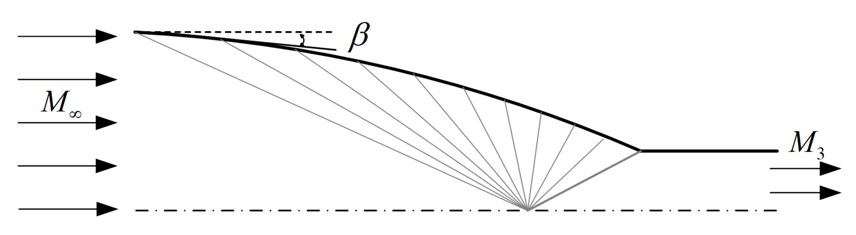
Figure 2.
Computing domain and structure mesh of a Busemann inlet.
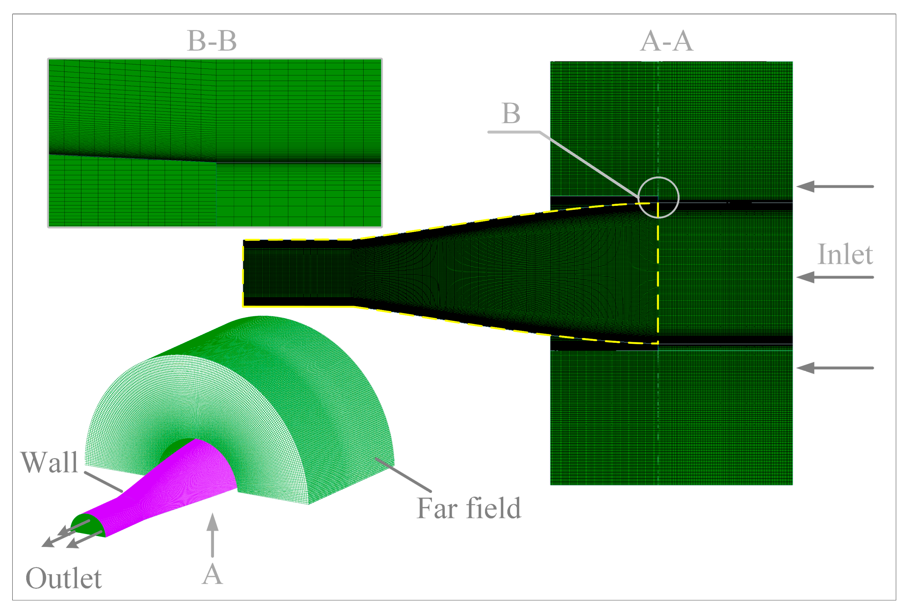
Figure 3.
Procedure of exergy postprocessing code with FLUENT UDFs.

Figure 4.
Grid independence verification.
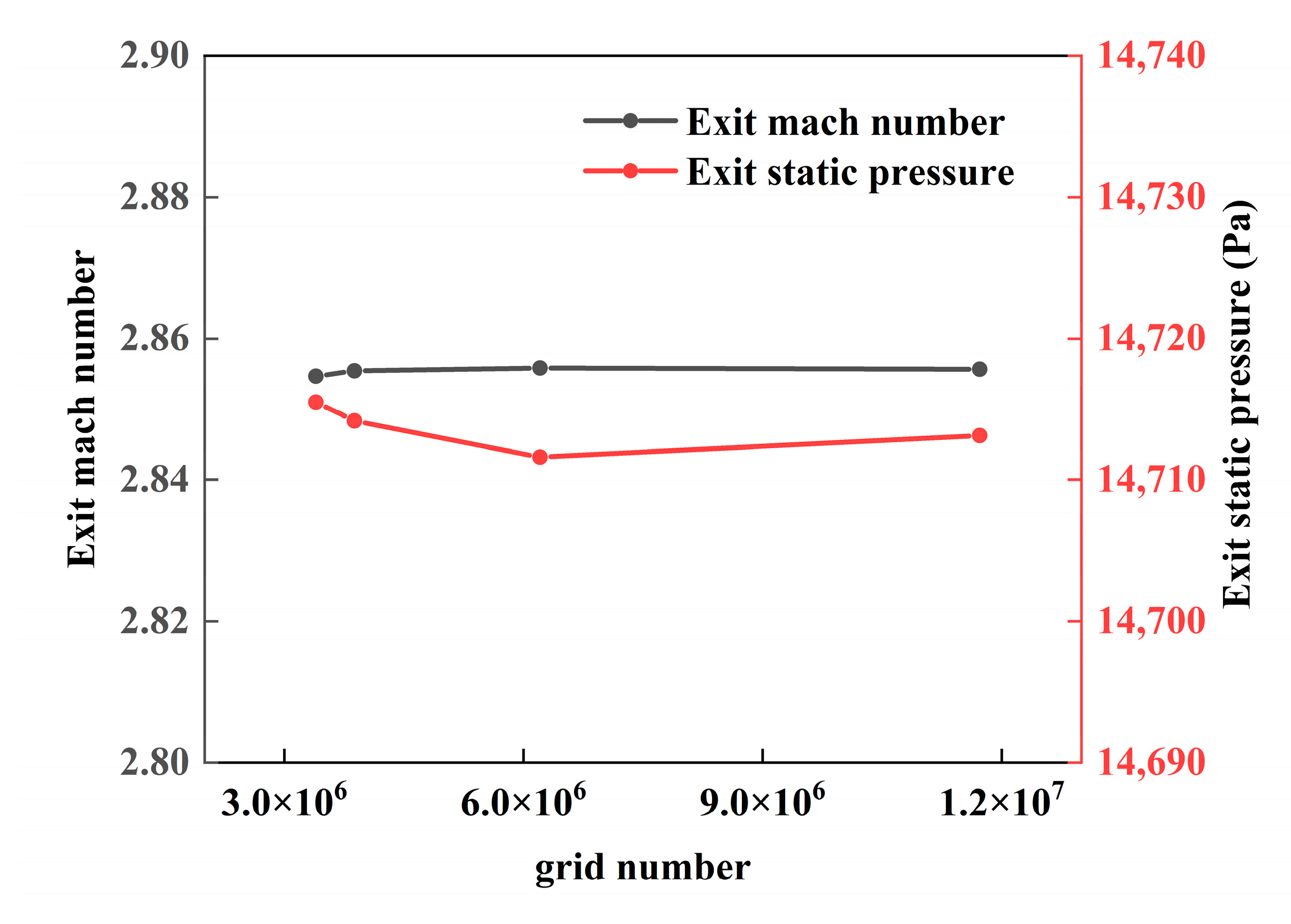
Figure 5.
Curves of distribution of Mach number along the wall.

Figure 6.
Mach number contours of inviscid flow in Busemann inlets.
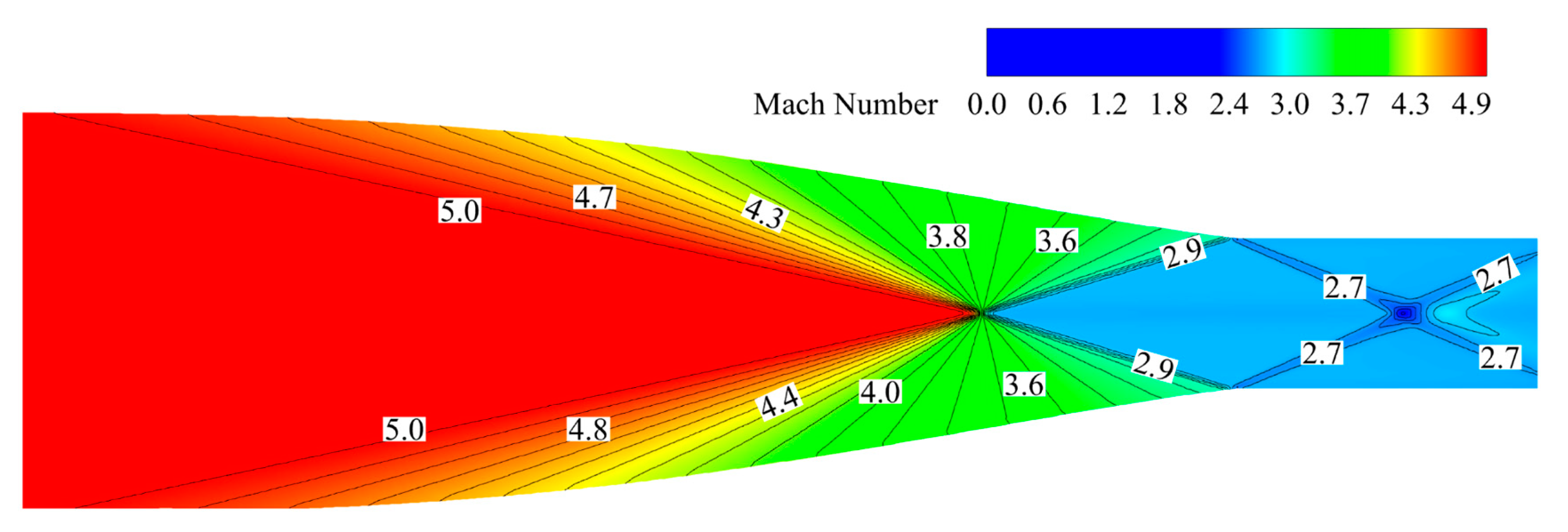
Figure 7.
Contours of entropy production of shock waves.

Figure 8.
Contours of Mach numbers.
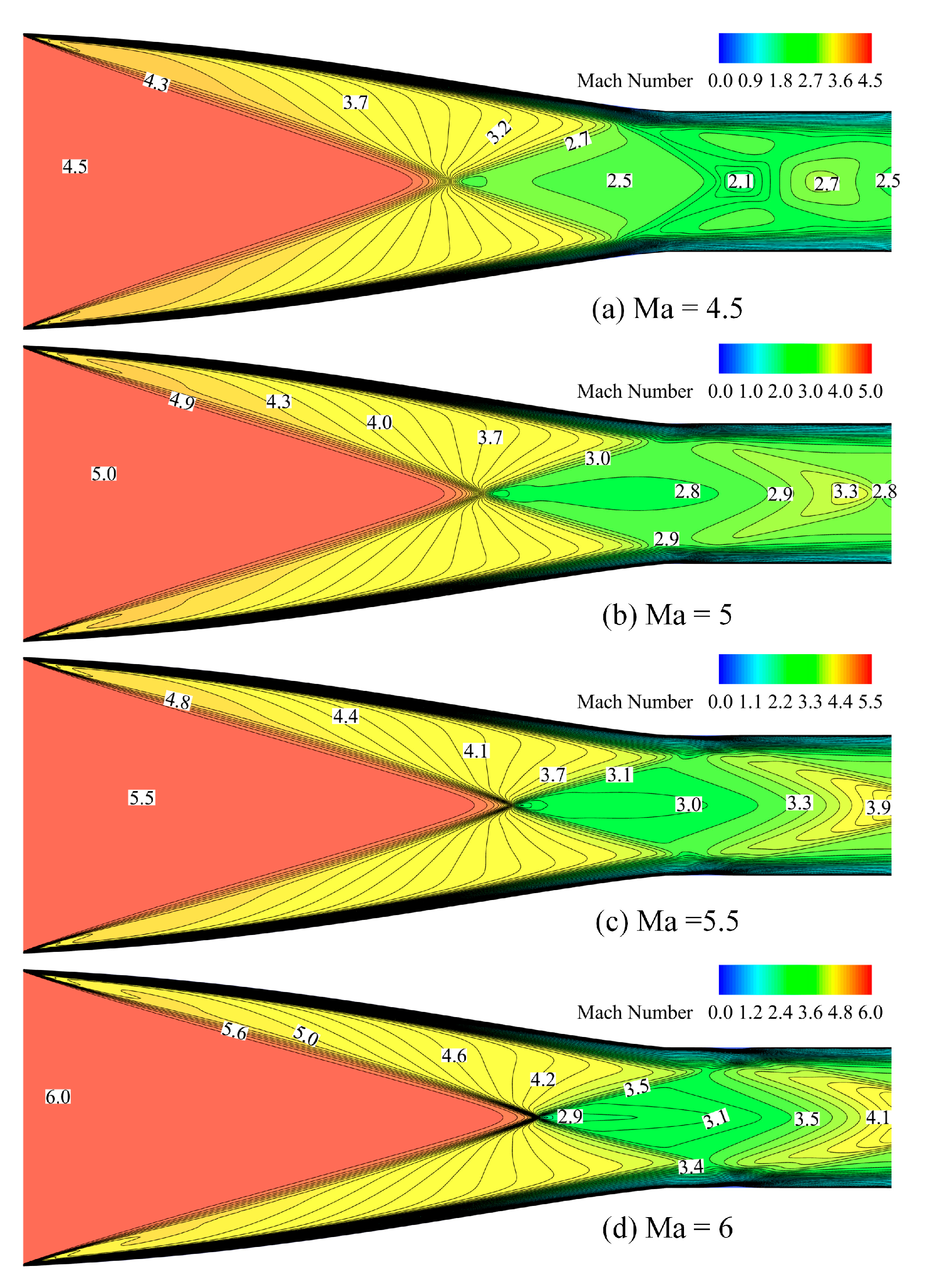
Figure 9.
Contours of total entropy production.
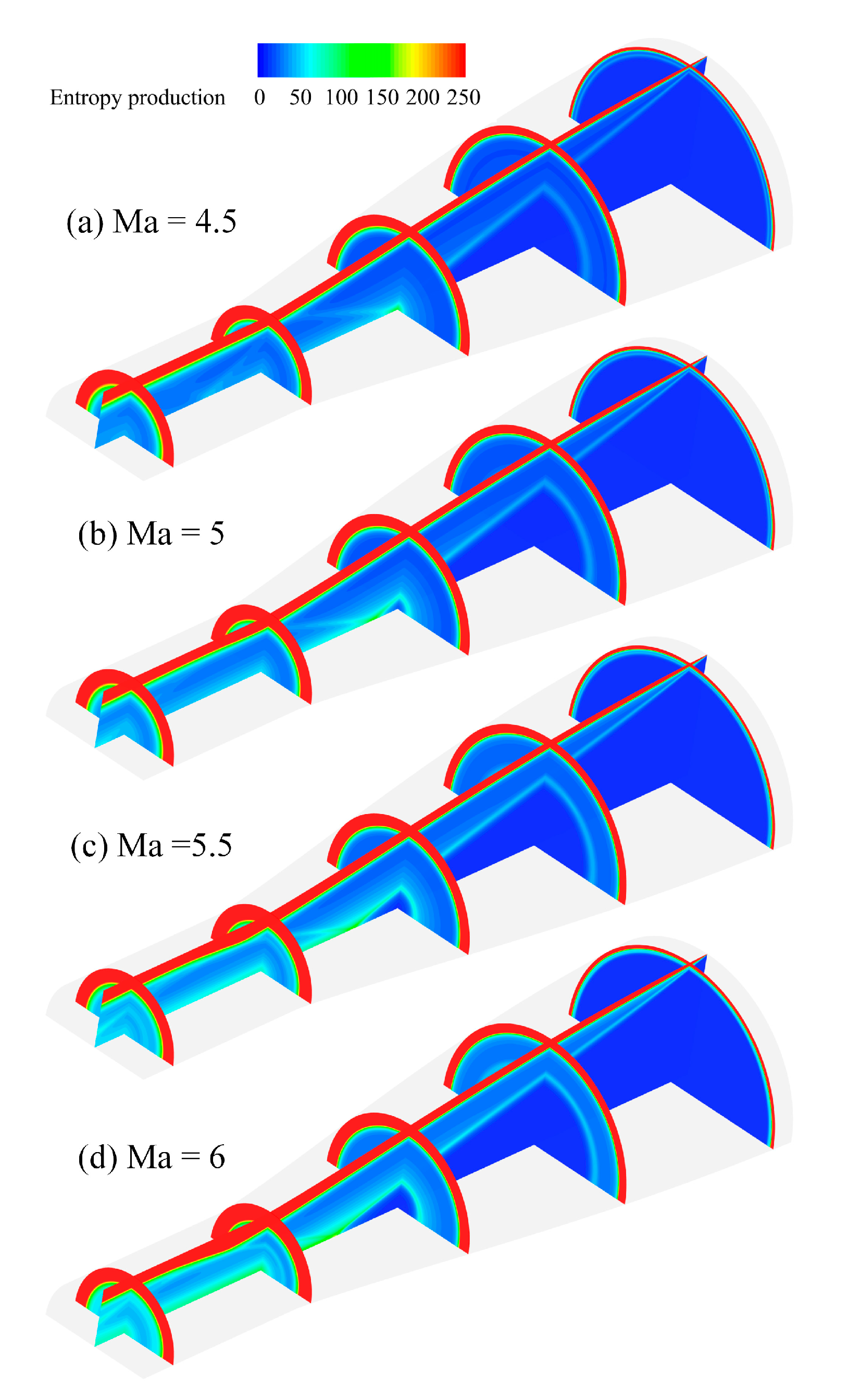
Figure 10.
Contours of shock waves’ entropy production.
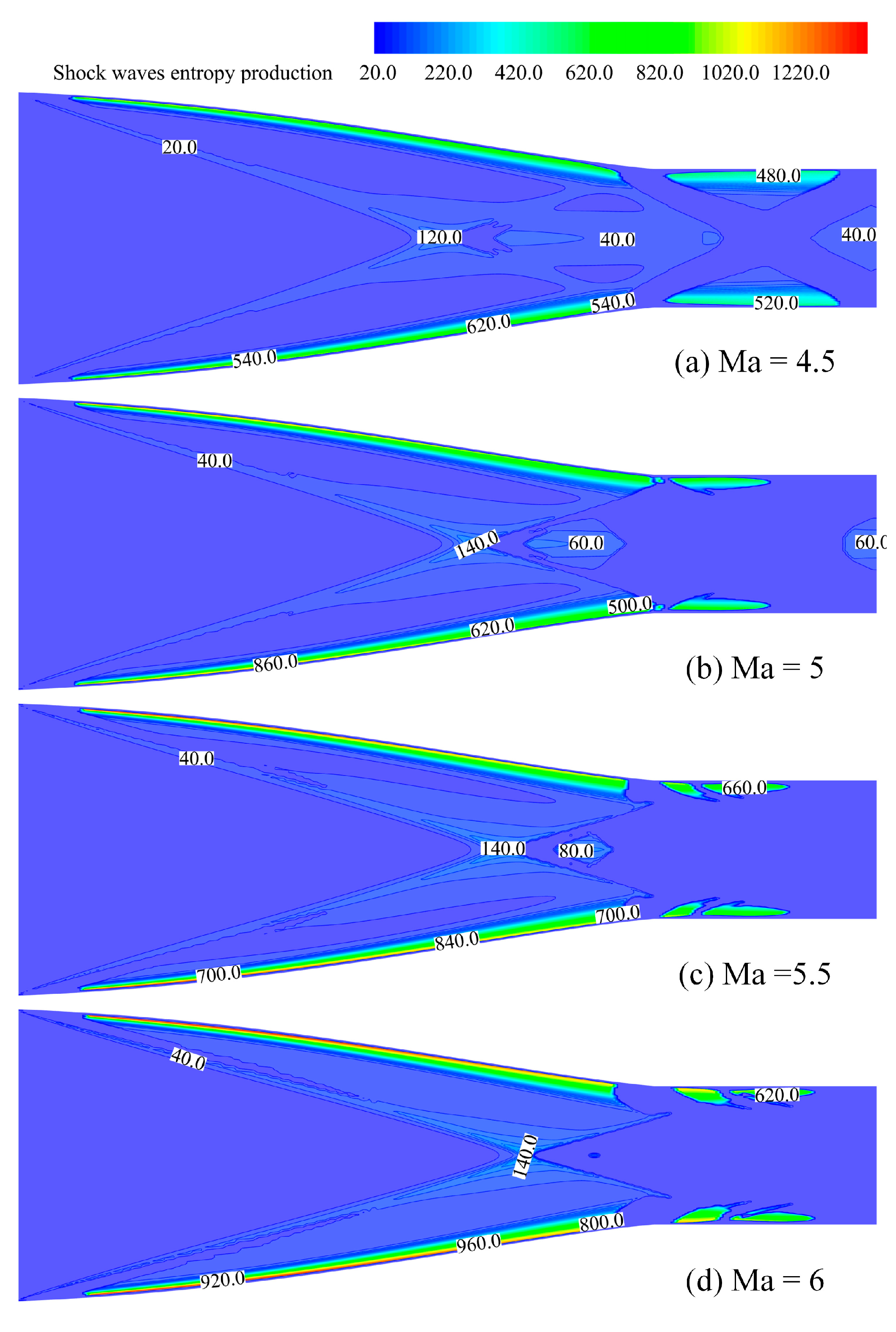
Figure 11.
Contours of thermal entropy production.
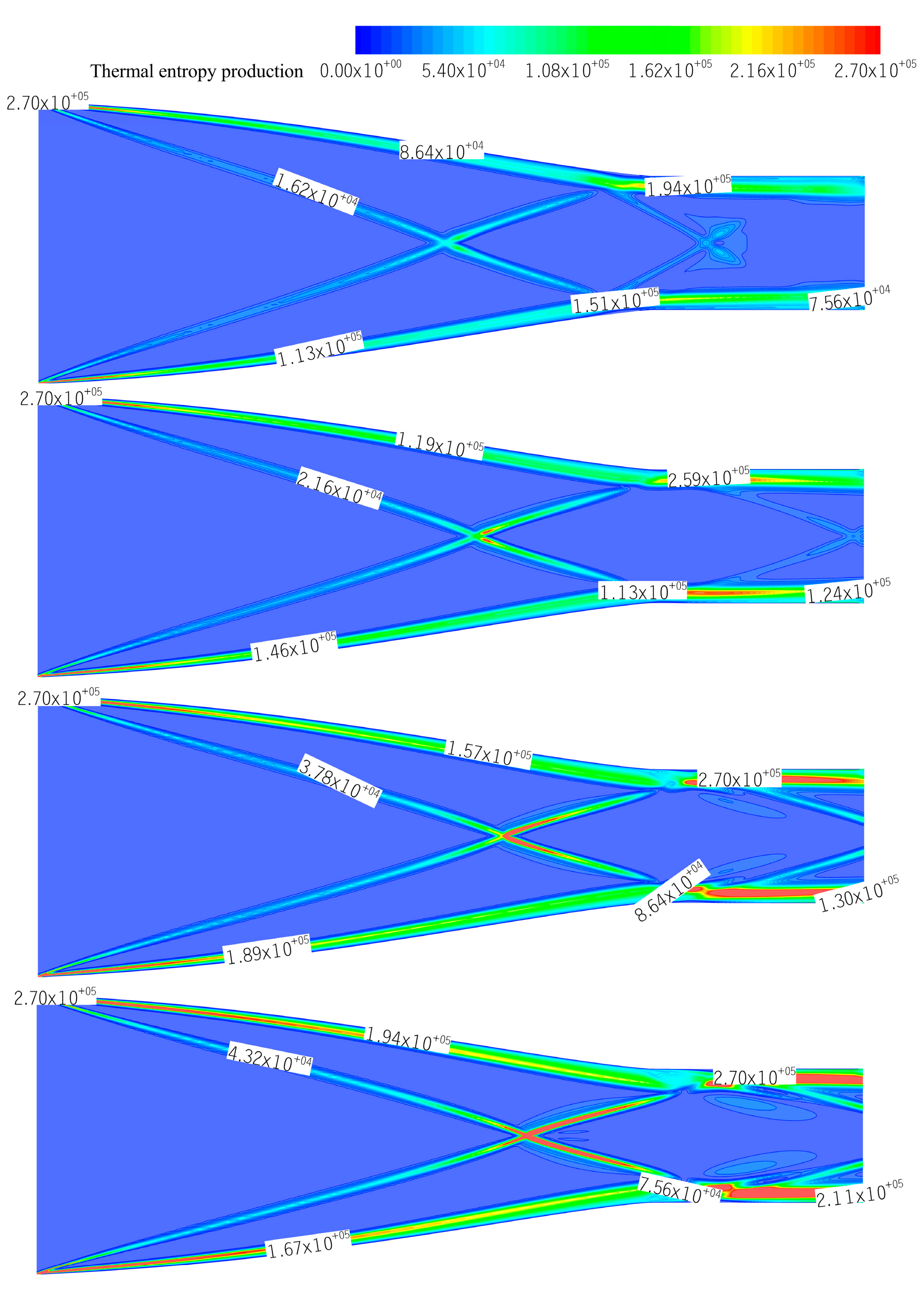
Figure 12.
Contours of viscous entropy production at four Mach number.
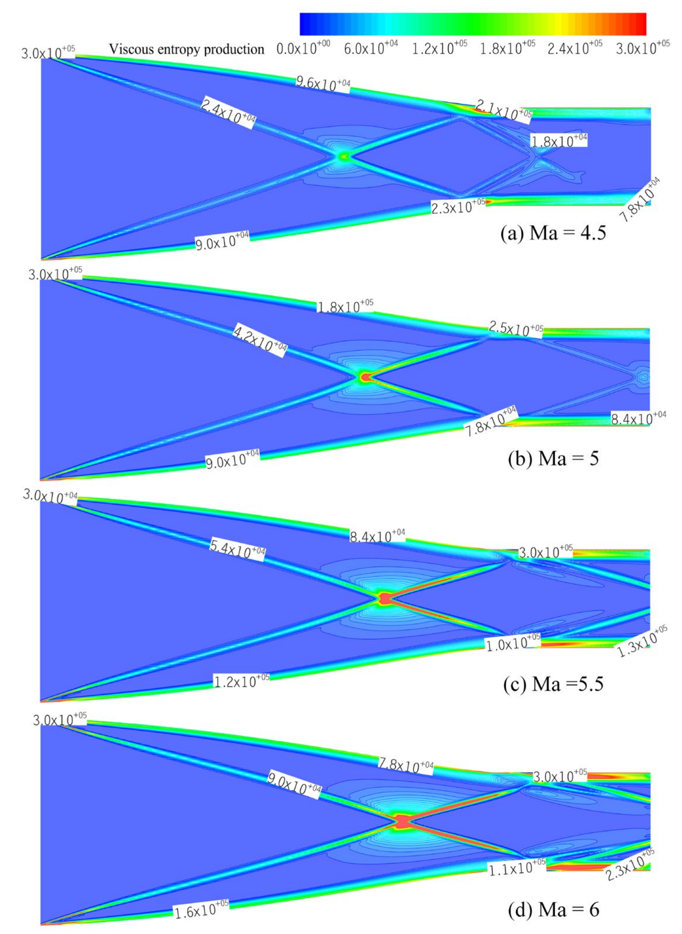
Figure 13.
Exergy destroyed decomposition in control volume of inlets.
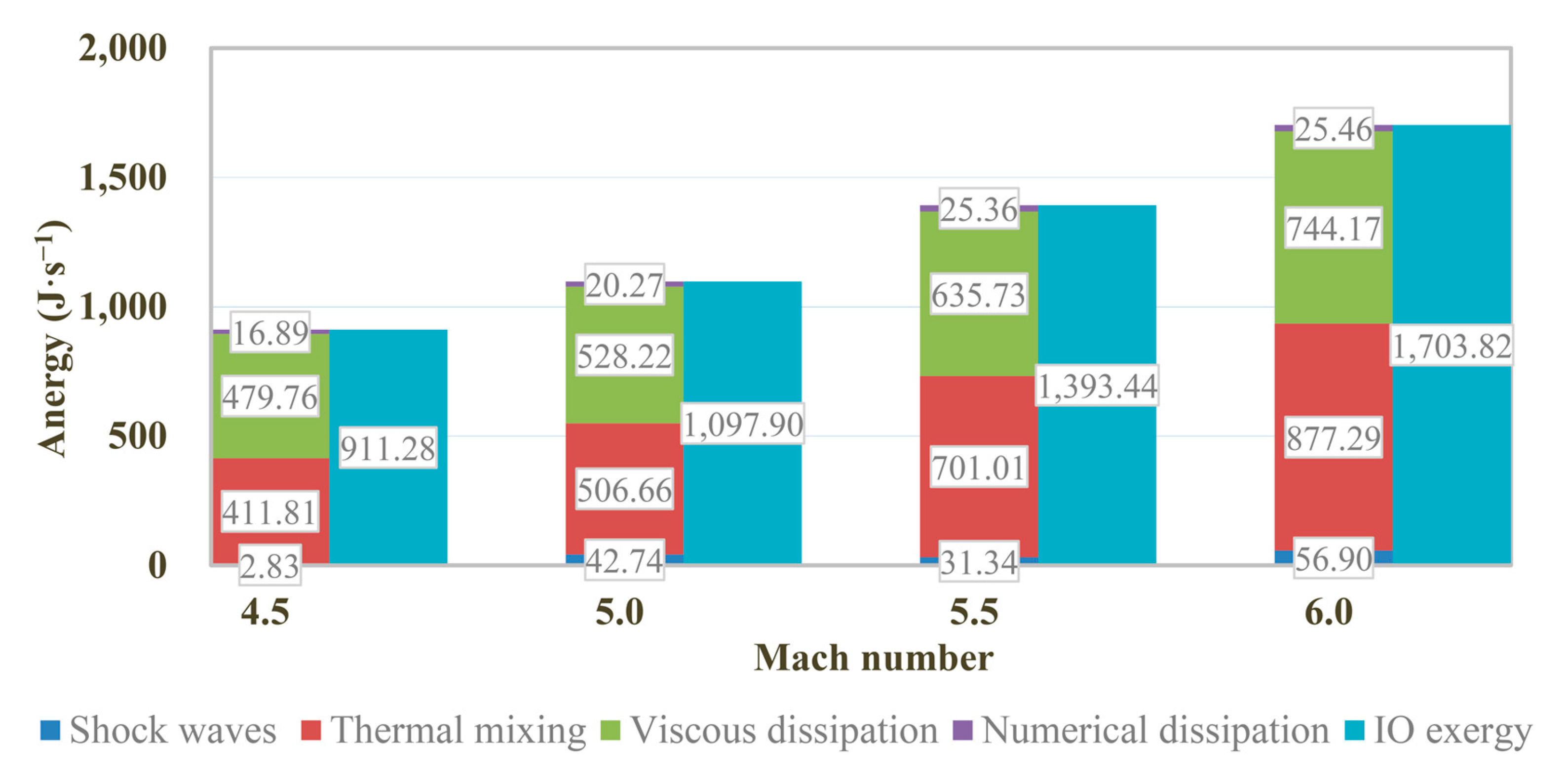
Figure 14.
Exergy stored in the entrance and exit of the control volume.

Figure 15.
Total pressure recovery coefficient and exergy destroyed efficiency versus flight Mach number.
Figure 15.
Total pressure recovery coefficient and exergy destroyed efficiency versus flight Mach number.
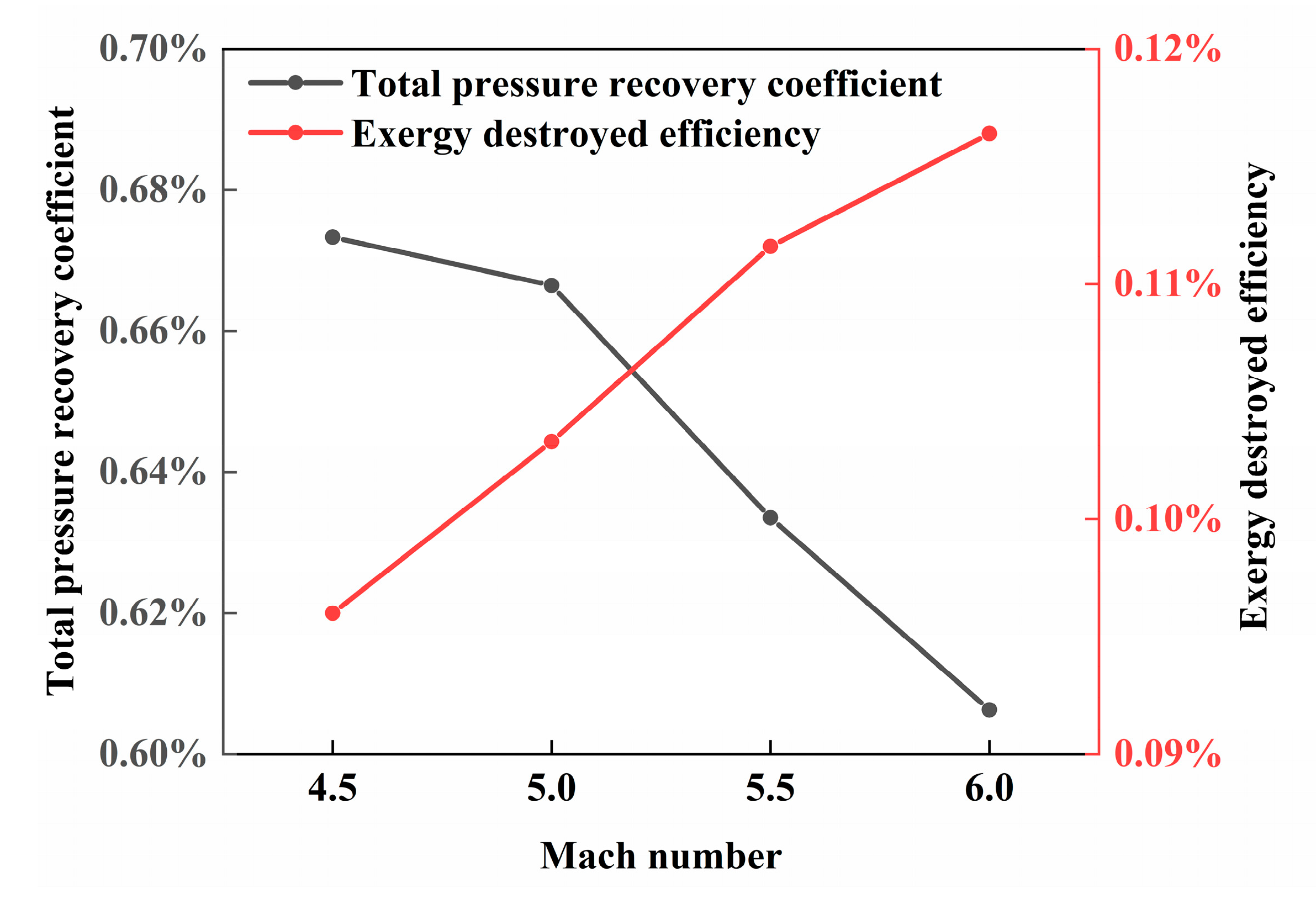
Figure 16.
Contours of total pressure recovery coefficient and entropy production at the cross section of outlets.
Figure 16.
Contours of total pressure recovery coefficient and entropy production at the cross section of outlets.

Figure 17.
Viscous anergy and thermal anergy versus flight Mach number.
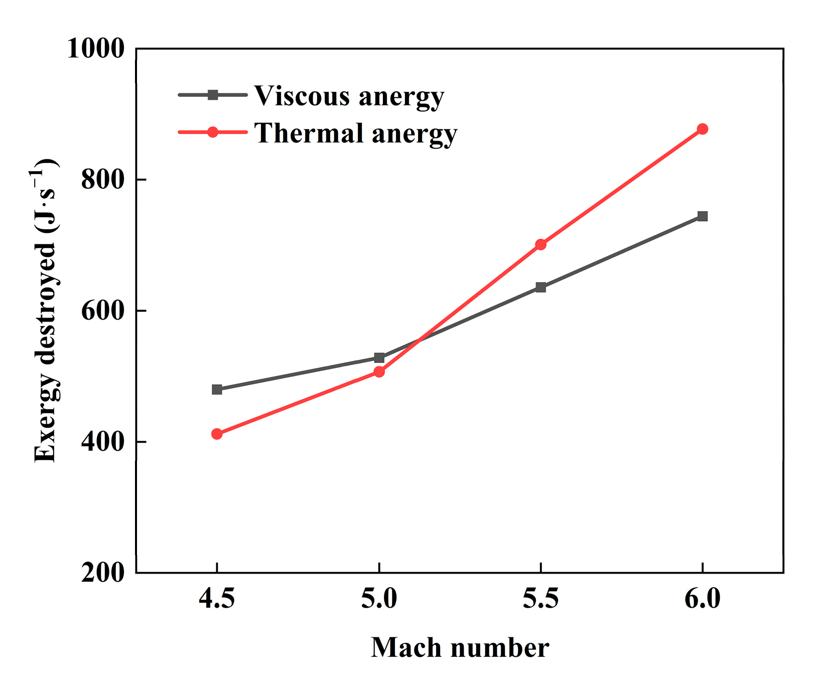
Figure 18.
Static pressure compression ratio and uniformity index versus flight Mach number.
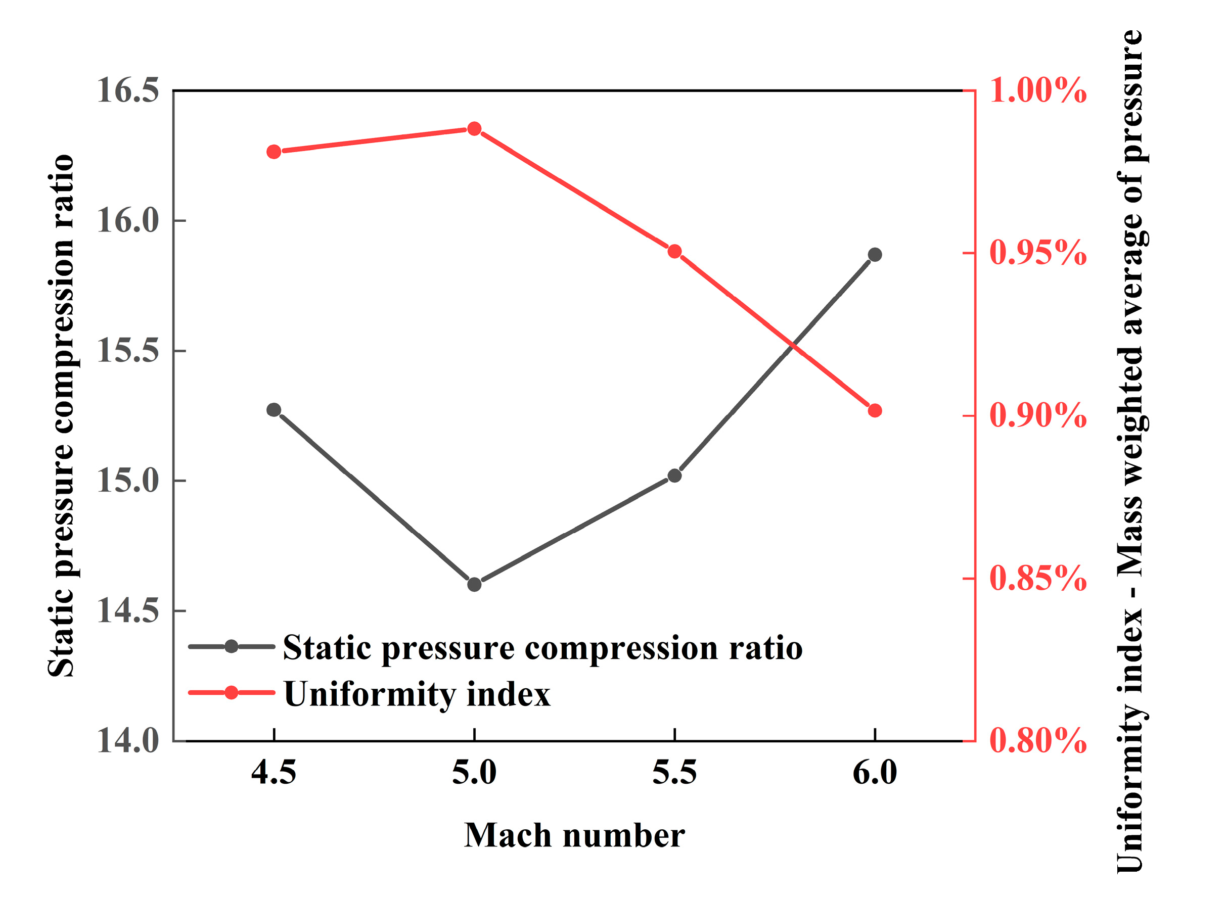
Figure 19.
Exit Mach number and static temperature ratio versus flight Mach number.


Table 1.
Physical and design parameters of Busemann inlets.
| Parameter | Symbol | Value | Unit |
|---|---|---|---|
| Freestream Mach number | 5 | − | |
| Throat Mach number | 3 | − | |
| Shape of exit | − | circle | − |
| Radius of exit | 10 | cm | |
| Ratio of specific heat | 1.4 | − | |
| Freestream pressure | 1170 | Pa | |
| Freestream temperature | 226.65 | K |
Table 2.
Comparison of anergy calculated from entropy production and balance equations.
| Entropy Production Rate (J∙K−1) | Anergy Calculated from Entropy (J∙s−1) | Anergy Calculated from Balance Equations (J∙s−1) | Errors |
|---|---|---|---|
| 0.189 | 42.84 | 42.93 | 0.21% |
Table 3.
Difference between the forms of exergy of the inflow and outflow.
| Parameters | Inflow | Outflow | Difference Value |
|---|---|---|---|
| Streamwise kinetic exergy deposition rate, (J∙s−1) | 34,742.70 | 25,274.78 | −9467.92 |
| Transverse kinetic exergy deposition rate, (J∙s−1) | 0.0 | 2.42 | 2.42 |
| Boundary pressure work rate, (J∙s−1) | 0.01 | 4449.84 | 4449.83 |
| Rate of thermal exergy, (J∙s−1) | 1986.71 | 6959.45 | 4972.74 |
| Total (J∙s−1) | 36,729.42 | 36,686.49 | 42.93 |
Disclaimer/Publisher’s Note: The statements, opinions and data contained in all publications are solely those of the individual author(s) and contributor(s) and not of MDPI and/or the editor(s). MDPI and/or the editor(s) disclaim responsibility for any injury to people or property resulting from any ideas, methods, instructions or products referred to in the content. |
© 2024 by the authors. Licensee MDPI, Basel, Switzerland. This article is an open access article distributed under the terms and conditions of the Creative Commons Attribution (CC BY) license (https://creativecommons.org/licenses/by/4.0/).
Share and Cite
MDPI and ACS Style
Zhu, M.; Zhou, S.; Liu, Y.; Li, Z.; Chen, Z. Control-Volume-Based Exergy Method of Truncated Busemann Inlets in Off-Design Conditions. Processes 2024, 12, 535. https://doi.org/10.3390/pr12030535
AMA Style
Zhu M, Zhou S, Liu Y, Li Z, Chen Z. Control-Volume-Based Exergy Method of Truncated Busemann Inlets in Off-Design Conditions. Processes. 2024; 12(3):535. https://doi.org/10.3390/pr12030535
Chicago/Turabian StyleZhu, Meijun, Shuai Zhou, Yang Liu, Zhehong Li, and Ziyun Chen. 2024. "Control-Volume-Based Exergy Method of Truncated Busemann Inlets in Off-Design Conditions" Processes 12, no. 3: 535. https://doi.org/10.3390/pr12030535
Note that from the first issue of 2016, this journal uses article numbers instead of page numbers. See further details here.