
The Splitter Blade Pump–Turbine in Pump Mode: The Hump Characteristic and Hysteresis Effect Flow Mechanism

1
Department of Energy and Power Engineering, Faculty of Metallurgy and Energy Engineering, Kunming University of Science and Technology, Kunming 650093, China
2
Department of Engineering Mechanics, Faculty of Civil Engineering and Mechanics, Kunming University of Science and Technology, Kunming 650500, China
*
Author to whom correspondence should be addressed.
Processes 2024, 12(2), 324; https://doi.org/10.3390/pr12020324
Submission received: 10 January 2024
/
Revised: 24 January 2024
/
Accepted: 31 January 2024
/
Published: 2 February 2024
Abstract
:This study focuses on the splitter blade pump–turbine as the research object to analyze the problems of hump characteristics and the hysteresis effect. We simulated the operation of the pump condition with small opening of the guide vane, analyzed the hydraulic loss by using the entropy production theory and entropy wall function, and investigated the study of internal flow transfer characteristics. In this paper, it was first verified that the maximum error of the energy loss calculated by the pressure method and the entropy production method was less than 6% for the working zone. From the quantified energy loss results, a significant instability feature was observed in the 0.65 QBEP–0.9 QBEP operating interval, accompanied by the phenomenon of the non-overlapping of the characteristic curves. The results show that the hump characteristic with hysteresis effect also exists in the splitter blade pump–turbine. The percentage of energy loss in the hump zone is in descending order of runner, guide vanes, spiral casing, and draft tube, but this changes again at low flow rates. By analyzing the high-entropy production region, it was found that the high-hydraulic-loss region is mainly distributed at the trailing edge of the long blade in the vane-less space, which is different from the traditional runner.
1. Introduction
Pumped storage units are characterized by a flexible start/stop, rapid response, and adaptation to rapid changes in system load through fast tracking, which results in rapid and frequent switching of the unit between pump and turbine modes, prolonging the operating time under extreme operating conditions [1]. Under the condition of a certain opening, the Q-H curve of the reversible pump–turbine with a low specific speed presents obvious hump characteristics, and the hysteresis effect occurs during the process of flow increase and decrease during operation (Figure 1). In the process of starting, stopping and regulating the flow of the pump, in the hump transition zone, an intense vibration will be produced, accompanied by a lot of noise, and the flow of the unit piping will be greatly oscillating. In serious cases, this will even cause the phenomenon of pump surge. Humping problems not only affect the safety, reliability and service life of the pump but also lead to operational failures of the unit [2]. The hysteresis effect also seriously affects the design of the hump safety margin, so it is necessary to actively explore the causes of the hump problem and hysteresis effect as well as optimization methods.
Factors such as rotational stall [3,4], backflow [5], secondary flow [6], cavitation [7,8,9], flow separation in the guide vane region [10], and geometrical parameters of the runner outlet [11] have an influence on the generation of hump characteristics. Numerous scholars have investigated the hump characterization of conventional reversible pump–turbines. Since the discovery of the hump characteristic by the Hydromechanics Laboratory of the Ecole Polytechnique Fédérale de Lausanne (EPFL) in 1998 when investigating the dynamic and static interference experiments between the guide vane and the runner [12], many researchers have found that the formation of the hump characteristic is closely related to the flow field [6,13]. Some scholars have found that chaotic internal flow conditions can cause the formation of hump zones [14]. Through the in-depth study of this finding, by means of simulation, some scholars [15,16] have pointed out that it is the change in flow separation intensity that causes chaotic internal flow conditions; Li [5] et al. believed that the main reason for the chaos of internal flow conditions is the backflow phenomenon at the entrance of the runner. On the experimental side, Guedes et al. [17] observed predominantly unsteady flow at the exit of the rotor through Particle Image Velocimetry (PIV) and Laser Doppler Velocimetry (LDV) tests, which presents inconsistent explanations in comparison with the results of the simulations. Another view is that the root reason for the hump zone is the rotational stall of the guide vanes [18,19,20], and other scholars have also found in their experiments that the rotational stall in the guide vane region is not the only root cause. Hump characteristics and hysteresis are also affected by the opening of the guide vane [21,22].
With the continuous deepening of research and innovation in methods, many scholars [23,24,25,26] have analyzed the internal flow and noticed that the formation of the hump zone and hysteresis phenomena is also correlated with the change in runner work and hydraulic loss. Under identical operating conditions, the hydraulic loss is different as a result of different discharge directions, different flow channel vortices and reflux states, and thus hysteresis effects.
In the past, when studying and analyzing the hydraulic loss of the pump–turbine, the overall performance of the pump–turbine is usually obtained using the differential pressure method, but it is difficult to determine the distribution and specific sources of hydraulic loss. More and more scholars have begun to link entropy production with hydraulic losses, and assess hydraulic losses relatively accurately by the type of distribution of entropy production. After Kock et al. [27] proposed the formula of the entropy production rate based on the Reynolds time-averaged equation and used it in the study of pipeline flow, the entropy theory has been gradually applied in the three-dimensional simulation of a pump turbine, vortex zone and other related fields of hydraulic machinery [28,29,30], and has made breakthrough progress. In the study of the hump phenomenon, some scholars have also adopted entropy theory to analyze the energy change [25,31,32], and considered that the high hydraulic loss of the hump area mainly originates from the return flow at the runner inlet, the high-speed circulation in the vane-less space, and the vortex in the guide vane. This shows that the entropy theory in thermodynamics can be used to analyze the instability characteristics of internal flow caused by the hydraulic instability of incompressible fluid in hydraulic machinery, which can achieve the purpose of accurately evaluating the hydraulic loss and precisely locating the loss position.
At present, the traditional reversible pump–turbines mostly adopt the form of a long blade runner. To improve the hydraulic performance of a pump–turbine, a new kind of runner, called a “split blade runner”, which uses long and short blades alternately in the circular direction, has attracted much attention in the world. Under high-head, high-flow operating conditions, pump–turbines with diverter vanes have superior hydraulic performance in this regard [33,34]. The use of long and short blade structures causes the rotor inlet leaf grid density to double, which can inhibit the occurrence of secondary flow inside the runner, improve the efficiency of the pump–turbine, especially the efficiency of the partial load, and significantly stifle the runner inlet de-fluxing and vortex phenomenon of the impeller channel. At present, the initial causes of the hump problem and hysteresis phenomenon of the conventional pump–turbine have been explored, but there is a lack of research on pump–turbines with splitter blades, and no scholars have elaborated on whether the hump characteristic and its accompanying hysteresis effect also exist, whether the causes of its formation are the same, and how it affects the stable running of the pump–turbine. Previously, the hysteresis phenomenon was not considered in the acceptance of a pumped-storage power plant. As a result, the analysis of the internal flow transmission characteristics and its correlation mechanism with energy loss is a key link to improve the hydraulic performance, reduce the pressure pulsation, and improve the stable running and efficiency of a pump–turbine. And it has become the key problem that needs to be solved urgently during the period of rapid development of the current pumped-storage energy.
In this paper, numerical simulations of a splitter blade pump–turbine are carried out to verify the hump characteristic and hysteresis effect. Firstly, by using the differential pressure method and the entropy theory to calculate the hydraulic losses caused by unsteady flow. Secondly, by exploring the variations in entropy production of the components in different directions. Lastly, the energy loss and its accompanying hysteresis effect leading to the hump characteristic are derived by analyzing the location of entropy production on the basis of the flow state.
This paper, firstly, introduces the entropy production theory and the entropy wall function; secondly, introduces the model building and its parameters, the selection of mesh and its division and the strategy of simulation; and, lastly, analyzes the results using the entropy theory and delineates other methods and conclusions.
The aim of this study is to find out the main components, the main locations and the main unsteady flow types of the reversible long- and short-vane pump turbine when it is running by pumping operation, so as to provide relevant references for the stable operation of the pump turbine as well as the setting of safety margins in the future.
2. Entropy Theory
2.1. Turbulent Entropy Production
In the formulation of the second law of thermodynamics, in a real system, there must be a power loss, resulting in entropy production. The hump characteristics and hysteresis effect of a pump–turbine are related to the energy losses of various components. In the internal flow of a pump–turbine, backflow, flow separation, vortex, rotational stall and other phenomena will lead to hydraulic loss, accompanied by an increase in entropy.
Equation (1) represents the local entropy generation rate [24]:
where represents the entropy production rate due to time-averaged movement; this can be expressed as follows [24]:
where represents the entropy production rate due to the velocity fluctuation; this can be expressed as Equation (3):
where μeff represents the effective dynamic viscosity of the fluid. This can be obtained from Equation (4):
When calculated using the RANS method, the components of the velocity fluctuation are not available, resulting in the entropy production rate due to velocity fluctuation also not being calculated. Kock [28] and Mathieu [35] showed that the local entropy production rate due to velocity fluctuation is related to ε or ω in the turbulence models; when the Reynolds number → ∞, there are relation (5) and (6) holds.
The local entropy rate of velocity fluctuation in the k-ε turbulence model can be expressed as
where ε is the turbulent dissipation rate.
The local entropy rate of velocity fluctuation in the k-ω turbulence model can be expressed as
Kock et al. [27] verified that this relationship is reasonable in turbulent heated channel flows.
2.2. Entropy Wall Function
Kock and Herwig [27,36] computed the local entropy generation rate using DNS and RANS. The results show that the entropy rate calculated by both methods is the same when the dimensionless distance y+ > 50. However, the velocity gradient is large and the wall entropy effect is strong in the wall region. Due to the severe underestimation of hydraulic losses caused by the poor resolution of the viscous substrate of the boundary layer, a method for solving the wall entropy production is by using the wall function. Remarkably, in their entropy wall functions, y+ is the only independent variable that can be regarded as not containing any computational result, and these entropy wall functions should not be confused with the wall functions of the flow solution.
In past calculations, wall effects have been ignored, or only the logarithmic region of the wall boundary layer has been considered, without considering the linear region adjacent to the boundary layer. As a result, hydraulic losses previously calculated using the entropy production theory were much lower than those calculated using the differential pressure method. Melzer changed the original form of the entropy wall function, and finally obtained the dimensionless entropy wall function in the mean flow state and turbulent state, as shown in Equations (7) and (8) [37]:
To obtain a dimensionless average of the wall entropy production , it is necessary to integrate the neighboring cells of the wall and then average through the characteristic lengths. For this study, we chose the first layer of the wall boundary layer mesh and the center of the mesh as the integration length and feature length.
The entropy production rate of the wall is shown in Equation (12):
From this, the main entropy production of the whole unit can be found:
where is the energy loss of the time-averaged movement, represents the energy loss of the velocity fluctuation, and denotes the energy loss of the wall effect.
Thus, the total energy loss can be obtained using Equation (16):
When the pump–turbine is in operation, the internal fluid is an incompressible fluid and the temperature of the flow is considered constant. Neglecting the hydraulic losses due to temperature changes, the localized volume hydraulic loss can be calculated by Equation (17):
When the pump–turbine is operating at pumping conditions, the hydraulic losses calculated by entropy production theory are transformed into hydraulic losses using Equation (18).
where hpro denotes the head loss; stands for the mass flow rate; and g is the acceleration of gravity.
3. Numerical Model and Schemes
3.1. Pump–Turbine Model
In this paper, a large-capacity, low-speed, high-head pump–turbine with a splitter blade was taken as the object of study. Table 1 lists the relevant parameters. The model machine was modeled in three dimensions using Solidworks 2020. The unit had a draft tube with an inlet hydraulic diameter of 562.5 mm, a spiral casing with an outlet diameter of 297 mm, a runner with a number of 5 long and 5 short blades each, 16 guide vanes and 16 stay vanes.
3.2. Numerical Schemes and Boundary Conditions
In this paper, a pump–turbine with splitter blade was modeled and numerically analyzed based on computational fluid dynamics. The Reynolds-averaged Navier–Stokes equations were calculated by the finite volume method. SST (shear stress transport) k–ω was chosen for the simulations. The SST k–ω model is most accurate in solving the flow near the wall. The low-Reynolds-number k–ω model is used for calculations in the boundary layer region near the wall, while the better-adapted high-Reynolds-number model k-ε is used for calculations in the free shear layer. It does not use the wall function, so it has better accuracy and stability in solving the flow in the near-wall zone. And it can accurately simulate the flow separation during the reverse pressure gradient, and more accurately simulate the complex flow field inside the pump–turbine. It has been verified that the SST k-ω model can accurately predict the hump of the pump turbine [30]. In this paper, the CFD of ansys fluent 2021 R1 was used to simulate the above model numerically. For the unsteady characteristics in head change, the velocity inlet and hydrostatic pressure outlet were used, the turbulence intensity at the inlet was set to 5%, and all the wall surfaces were defined to be smooth and non-slip. To obtain a more accurate hump characteristic curve and hysteresis phenomenon, the calculation results of the previous operating point were set as the initial boundary conditions of the next operating point during the simulation calculation. In the calculations, it was assumed that the full range of conditions had negligible temperature changes, there was no distortion of the calculations in the transition section due to flow changes, and that the liquid water in the flow channel was incompressible.
3.3. Grid Independence Validation
The computing domain consists of five parts: the draft tube, the runner, the guide vane, the stay vane and the spiral casing, as in Figure 2. We shared the topology of the components so that the interfaces of the components were set up as fluid interior surfaces. Considering the limited computational resources, the polyhedral mesh was finally selected. Because this form of mesh was chosen to reduce the number of meshes, the mesh quality was also superior to tetrahedral meshes overall. Since each grid cell has more faces, it is possible to make each cell have more neighboring cells, and such a grid form can effectively improve the accuracy of the gradient calculation. The minimum mesh size was selected as 2.5 mm and the maximum mesh size was set to 40 mm for the polyhedral mesh, as shown in Figure 3. To make the flow field data more accurate, the mesh close to the wall needed to be encrypted and refined; with the boundary layer added to all walls, the average value of y+ was less than 1.5. We achieved a convergence of the residuals for all parameters at the time of calculation of less than 10−3, and even at the minimum flow rate this criterion reached 10−2, and the difference between the monitored inlet and outlet flows was less than 0.5%.
To ensure the accuracy and precision of the calculation results, a validation of the independence of the grid is required to evaluate the energy, efficiency, and torque for the full operating conditions by adjusting the number of nodes. A total of three sets of grids were designed for this study, as shown in Table 2. The dimensionless energy coefficients EnD, torque coefficients TnD, and efficiency η were chosen as the reference for verification according to the International Standards Committee (IEC). From Figure 4, it can be observed that the energy, efficiency and torque errors were less than 5% for each operating point when the number of cells was greater than 11 million. For the design workspace, the maximum error was only 4.13% for the energy coefficient End and 6.08% for the efficiency η. Therefore, we considered the simulation calculations in this study to bereasonable and credible.
4. Analysis of Numerical Results
4.1. Characteristic Curve of Flow Head
It has been found that the hysteresis characteristics of a conventional pump–turbine are particularly pronounced at the smaller openings of the guide vane [31]. In this study, to obtain a more pronounced hump and hysteresis phenomenon of the splitter blade pump–turbine, the GVO was calculated with a setting of 23 mm for all operating points. To obtain the hysteresis characteristics of the Q-H curve, the simulation of dozens of operating points was used for the results of the previous operating point and for the next operating point of the initial boundary conditions for the calculation, considering that the hump area generally only appears when the pump working condition is small flow, and the conventional pump–turbine often appears in 0.6 QBEP–0.9 QBEP [7,21,24,38,39]. We designed the operating conditions, selected as 0.3QBEP–1.3QBEP. The method used was as follows: The flow rate of the optimal operating point (QBEP) was used as a benchmark. We simulated the calculations of the pump conditions and the operating flow rate in the 0.31 QBEP to 1.3 QBEP interval, respectively. We simulated the flow rate in the direction of the increase (Inc) and calculated the minimum flow rate from 0.31 QBEP to the start, and then gradually increased the flow rate and calculated the maximum flow rate of 1.3 QBEP. Finally, in the direction of flow decrease (Dec), the simulation was started from the point of maximum operating conditions, and then the flow was gradually reduced and calculated to a minimum flow of 0.31 QBEP. In the calculation process, each working point had the same parameters and boundary conditions, except the initial flow field state was different.
Figure 5 shows the flow-head characteristic curve obtained from the steady-state simulation calculations at 23 mm GVO for the splitter blade pump–turbine. We divided all work regions into a low-flow area (0.31 QBEP–0.63 QBEP), a hump area (0.63 QBEP–0.9 QBEP) and a high-flow area (0.9 QBEP–1.3 QBEP).
4.2. Calculation of Hydraulic Losses
For the energy loss calculation of the hydraulic machinery, the traditional way uses the pressure difference between the inlet and outlet of each component to calculate its energy loss. For the pump–turbine, Equation (19) was used to calculate the energy losses in the draft tube, guide/stay vanes, and spiral casing parts. The hydraulic loss in the runner is the difference between the total rotation input work and the work obtained by water pressurization, and can be calculated using Equation (20):
where h∆P represents the head loss calculated using the pressure method, pTot denotes the total pressure of the fluid particles, and Ws is the runner input work of the pump–turbine in the pumping mode.
In order to verify whether the energy loss calculated by the entropy production theory is correct, the total energy losses hpro calculated by the entropy production method for each operating point was compared with the total energy losses calculated by using the differential pressure method for h∆P. As shown in Figure 6, the maximum error between the hydraulic losses calculated by the pressure method and the entropy production method in the direction of increasing flow was 8.62%, which appeared in the low-flow working area, the error at the optimal working point was −1.51%, and the errors of the results of both calculation methods in the hump area and the high-flow working area are within 5%. As shown in Figure 7, the maximum error between the hydraulic loss, calculated by the differential pressure method, and the hydraulic loss, calculated using the entropy production method, was −11.3% in the direction of decreasing flow rate, which also occurred in the low-flow operating zone, with an error of 5.25% at the optimum operating point.
Through the error comparison analysis, it can be seen that the maximum error of the head loss occurred in the small-flow working area, and this value was also less than 6% near the optimal working condition point, which indicates that the head loss calculated by the entropy production method is in good agreement with the head loss calculated by the differential pressure method. The hydraulic losses calculated by the entropy generation method were proven to be reasonable and credible.
The hydraulic loss of the whole unit can be divided into the entropy production in the main flow area and the entropy production in the wall area by using the entropy production method. The wall entropy production is mainly caused by the large velocity gradient due to the shear stresses between the first layer of mesh nodes and the wall, which can be approximated as friction loss. Entropy production in the main flow region is caused by changes in velocity gradients due to flow separation, reflux, shocks, vortices, etc. The proportions of entropy production in the wall-region hydraulic loss (hpro,W) and the main-flow-region hydraulic loss (hpro,A) in both directions of flow increase and flow decrease are given in Figure 8.
There was no significant change in the entropy production in the wall zone with the change in flow in both the increasing and decreasing directions, while the hydraulic loss due to the entropy production in the main flow zone in the interval of 0.65 QBEP–0.9 QBEP in both directions showed an obviously unstable region. The comparative analysis showed that the hump characteristic was mainly caused by the hydraulic loss due to the unsteady flow in the main flow zone, and had little to do with the hydraulic loss due to wall friction.
The entropy production rate of each component of the unit for each working condition is shown in Figure 9, from which it can be seen that the entropy production rate of the draft tube was very small in the design working region, but in the case of the small flow rate, the entropy production rate of the draft tube started to increase gradually as the flow rate ratio decreased until it was close to the entropy production rate of the spiral casing. In the entropy production share of each component of the unit at each operating condition, the entropy produced by the runner and the guide vane always dominated.
In the analysis of the entropy production of the full working condition, it can be seen that the entropy production of the two components, the runner and the guide vane, was always dominant as the flow rate changed, and the hysteresis phenomenon occurred in the hump area. In summary, the pump–turbine with the splitter blade, in pump mode, also had a hump characteristic and was accompanied by a hysteresis effect. By calculating and analyzing the hydraulic loss, this phenomenon was mainly caused by the hydraulic loss due to the unsteady flow inside the runner and the guide vane, and the hydraulic loss in the wall area had little effect on it.
5. Detailed Distribution of Local Entropy Production Rate
To reveal the flow mechanism of the hump area and hysteresis characteristics of the splitter blade pump–turbine, it was necessary to further analyze the correlation mechanism between the hydraulic loss and flow change in each component under different working conditions, and to obtain the rule of change between the entropy production distribution of the unit and the hump characteristics. In the flow-head curve relationship of Figure 5, it is clearly found that in the flow rate 0.65 QBEP–0.9 QBEP interval, there was a hump zone, accompanied by a hysteresis phenomenon. According to the above analysis, the main reason for this phenomenon is the hydraulic loss of the main flow zone of each component. To investigate the causes of hump characteristics and hysteresis effects in the splitter blade pump–turbine, the local entropy production rate (LEPR) distribution of each component needs to be analyzed. During the analysis of the local entropy production, it was assumed that the change in the value of the wall entropy production in different flow directions had a negligible effect on the hysteresis effect.
5.1. LEPR Distribution in the Runner
Figure 10a–f represents the entropy production distributions for the 1.15 QBEP, 1.00 QBEP, 0.81 QBEP, 0.73 QBEP, 0.63 QBEP, and 0.38 QBEP working conditions. Due to the small-flow operation, the blade inlet impulse angle was larger, resulting in the blade inlet being prone to water impingement, de-fluxing and vortex shedding, and the energy loss being larger. Therefore, different unfolding surfaces at the blade inlet (cylindrical sections SP0.95, SP0.8 and SP0.5 with different interceptions at the leading edge of the long blade) were selected to analyze the entropy production distribution between the crown and the band of the impeller blade inlet in order to assess the hydraulic losses in the blade inlet and the flow channel.
At the working condition point 1.15 QBEP, the water flow pattern in the flow channel was more stable, the flow line was uniform and smooth, and the pressure in the rotor channel was symmetrically distributed in the circumferential direction, which gradually increased from the inlet to the outlet. From Figure 10a, it can be seen that the LEPR distribution of the three unfolded surfaces was mainly concentrated at the position of the inlet at the leading edge of the long blade, as shown in Region I and Region II in Figure 10. The two regions were locally enlarged, and the velocity vector diagrams were conducted to analyze the flow pattern, and it can be seen that Region I was generated by the flow separation leading to the low-speed disturbance, which caused the hydraulic loss, and Region II was the fluid with a large change in velocity gradient, which led to the high hydraulic loss and the formation of vortex-like streamlines at the local level. The distribution of the high LEPR in the two discharge directions was almost the same.
At operating point 1.00 QBEP, the region of high entropy production near the inlet decreased dramatically, but the region at the leading edge of the blade pressure remained. At 1.0 BEP, the impulse angle between the blade mounting angle and the inlet airflow angle was small; therefore, the flow separation was not severe and the hydraulic losses were minimized. The distribution of high LEPR area was also the same in both discharge directions.
In the direction of flow increase, at 0.81 QBEP, the impulse angle between the blade mounting angle and the inlet airflow angle increased due to the smaller flow rate, the flow separation phenomenon was intensified, and the water flow at the blade inlet position was impinged, causing the water flow to become unstable. As a result, the overall high LEPR area increased, and the main high LEPR area still occurred at the leading edge of the suction surface and produced a band-like LEPR area at Region III, which can be seen from the velocity vector diagram of this area, due to the presence of the return flow at the inlet of the runner, which generated an unstable, low-speed disturbed flow that spread backward, and, after passing through the leading edge of the short blades, it was again affected by the short blades, so that the disturbed flow passed on to the next foliation, resulting in hydrodynamic losses, and thus producing a band-like high-LEPR area. However, in the direction of flow decrease, there was no banded hydraulic loss area. By comparing the entropy production distribution in the two directions, it can be clearly seen that in the direction of flow increase, the total entropy production at this condition point was obviously different from that in the direction of flow decrease. This infers that the presence of backflow at the inlet of the leading edge of the runner long blades causes an unsteady flow pattern, which produces different hydraulic losses due to different distributions and intensities, giving rise to the hump characteristic and hysteresis effect.
In the direction of flow increase, 0.73QBEP, the water flow at the inlet entered the blades at a large deflection angle, due to the large gap between the two blades at the inlet of the splitter blade runner. The pressure at the inlet showed an uneven distribution in the circumferential direction, and there was a reflux and a stronger flow separation phenomenon in the hub area near the runner inlet. The high LEPR areas of Region IV and Region V were generated in the leaf channel, and it can be seen by analyzing the velocity vector map of this region that both regions were due to the low-speed turbulence, which caused an unstable flow condition, and consequently higher LEPR. And there was no large region of high entropy production in the direction of flow reduction. This directly affected the hump characteristics and hysteresis effect of the diverter vane pump–turbine.
It decreased continuously from 0.73QBEP to 0.63QBEP, and the high LEPR areas were mainly concentrated at the inlet of the runner, where the blade’s leading edge is located. When the operating conditions were at 0.38QBEP, the water flow in the blade inlet deflection angle was greater, the runner inlet near the hub area of the phenomenon of reflux, de-fluxing phenomenon was intensified; the impact loss became more and more intense, and, due to the role of the runner accelerating and twisting, in the case of the small flow of the conditions, the water flow in the runner had more areas of large gradients in flow velocity, leading to more chaotic flow and a greater spread of entropy production areas in bands. In the direction of flow increase, the region near the wall of the long and short blades, there also appeared a wide range of high hydraulic loss areas; this is due to the fact that away from the design working condition point, the fluid flow in the impeller channel was very irregular, resulting in the fluid and the blade impact and friction loss, and the fluid in the rotating parts being insufficiently developed, resulting in the hydraulic loss.
5.2. LEPR Distribution in the Guide/Stay Vanes
In the entropy production share diagram of each component in Figure 9, it can be seen that the entropy production share of the movable guide vane component was second only to that of the runner, and through the entropy loss results, it can be found that in the flow rate of the 0.6 QBEP–0.9QBEP interval, the hump characteristic and hysteresis effect obviously appeared in the splitter blade pump–turbine.
To analyze the flow pattern and LEPR distribution of the water flow inside the movable guide vanes and to investigate the development trend of the water flow inside the downstream components, Figure 11a–f shows the distribution of the LEPR for each operating point of the guide vanes/stay vanes and the spiral casing in different directions. The two flow conditions of 1.15QBEP and 1.00QBEP were analyzed first, as shown in Figure 11a,b. It can be seen that the high LEPR area was mainly located in the wake region of the guide vane and the flow channel between the guide vanes. We performed flow regime analysis of Region I, II, and III for high LEPR. At Region I, the friction influence of the guide vane wall produced the phenomenon of low-speed turbulence, resulting in large energy loss; at Region II, vortices were generated on the suction side of the guide vane due to small opening operating conditions, influenced by the leading edge of the vane. However, at the exit of the runner, there was a region of high LEPR. From the velocity vector diagram, it can be seen that the higher LEPR are was, distributed in the exit of the long blade, while the exit of the trailing edge of the short blade did not appear in the high LEPR area; this feature was different from the conventional pump–turbine blade runner, which suggests that the unsteady flow pattern may only occur in the exit of the trailing edge of the long blade. Although the distribution of LEPR was slightly different for each operating point in different directions within the design work area, the overall hydraulic losses were almost the same.
Figure 11c–e shows the LEPR distributions in different directions for the 0.81QEBP, 0.73QEBP, and 0.63QEBP operating points. All the operating points were located in the hump area and in the hysteresis loop, because with the pump–turbine in low-flow operation, the back of the guide vane fluid is prone to flow off the negative pressure phenomenon. And because the guide vane is a small-opening working condition with the fluid going into the guide vane channel, the guide vane inlet fluid incidence angle is larger, and the fluid flow through the guide vane will produce a large bending and rotating, thus increasing the fluid’s kinetic energy loss and vortex loss and resulting in a reduction in efficiency. From the figure, it can be seen that from the 0.81QEBP operating point to the 0.63QEBP operating point, the main high LEPR area developed from the foliation-free area of the runner and the guide vane to the gap between the guide vane and the stay vane, and not only did the area of the hydraulic loss increase, but the overall hydraulic loss also increased. After the flow became smaller, at the spiral case nose, there was an obvious high-LEPR area in Region IV. By analyzing the flow pattern near the spiral case nose, it was found that this is due to the water flow and spiral case nose inlet leading edge of the impingement resulting in flow chaos, and with the fixed guide vane trailing edge at the unstable flow of each other resulting in a larger hydraulic loss. And compared with the optimal working condition point, the entropy production in the wake region of the guide vane increased significantly, and two high-LEPR areas of region V and VI appeared. By analyzing the velocity vector diagram, Region V is a high-LEPR area due to the combination of the wake effect around the trailing edge of the guide vane and vortices generated by flow separation, significant flow separation occurs in Region VI, where severe momentum exchange occurs between the low-velocity region and the high-velocity secondary flow in the adjacent channel, resulting in transport effects, which leads to high hydraulic losses. In addition, as the flow rate increases, the vortices at the suction surface and the mismatch described above become more pronounced, and the chaotic flow characteristics will have a greater impact on the hydraulic losses. And the degree and location of flow separation in the two directions were significantly different, further forming separation vortices in some areas, clogging the channel and interfering with the normal flow of water through it. Consequently, the increase in velocity in neighboring channels leads to different degrees of momentum exchange, causing different hydraulic losses.
At the low-flow operating point 0.38 QEBP, the impulse angle of the incoming flow becomes larger, and the water flow impacts violently with the inlet of the guide vane, resulting in the vane-less space between the runner outlet and the guide vane as a high-LEPR zone. This is due to the intense evolution of the flow channel vortex and flow separation, and in the leading edge of the guide vane inlet position by the inlet surge, the water flow and the guide vane wall impingement, a variety of flow patterns once again interfere with each other, leading to the guide vane between the flow channel received by the serious blockage. As a result, momentum exchange increases, leading to an increase in the region that brings about high-LEPR area.
In conclusion, whether at the design operating point, the optimal operating point or at the far optimal operating point, the hydraulic loss between the guide vanes is mainly caused by the unsteady water flow at the outlet of the runner’s long blade and the flow separation, and the separation vortex that occurs in the channel of the guide vanes. And in different directions in the high-LEPR region, distribution is different, resulting in different energy losses, the splitter blade pump condition of the flow-head curve hump characteristics and the formation of the hysteresis effect.
5.3. LEPR Distribution in the Draft Tube
This is evident from the plot of entropy production share for each operating condition in Figure 9: the entropy production within the main flow zone in the draft tube remained almost unchanged for the high flow conditions 1.0QBEP and 1.15QBEP. In the hump zone, the LEPR was only slightly different in both directions, and the LEPR in the main flow zone of the draft tube increased with decreasing flow only for the small-flow conditions 0.63QBEP and 0.38QBEP and occupied a somewhat larger share. Thus, in both directions, the hydraulic losses in the draft tube have only a slight influence on the generation of hysteresis effects.
Three cross sections, A-A, B-B, and C-C, were selected in the straight conical section of the draft tube to observe the trend and distribution of LEPR in the three cross sections, as shown in Figure 12. As can be seen from the figure, the region of high LEPR at low flow conditions spread up to the C cross-section. Figure 12 shows the entropy production distribution of each cross-section at each working condition point in different directions. It can be concluded that none of the high-LEPR areas exist in the main flow area of the draft tube in the high-flow work area due to the relatively more stable flow. When the flow decreased to 0.81QBEP and 0.73QBEP, high-LEPR areas appeared in the A-A section in both directions, but there were higher-LEPR areas in the direction of increasing flow than in the direction of decreasing flow. This is because when the pump–turbine is operated at these operating points, backflow occurs in the wall area near the A-A section of the draft tube outlet, resulting in different energy losses in the two flow directions. As flows continue to decrease, backflow intensifies and the high-LEPR area expands further. A relatively high LEPR zone was also observed in the C-C section at the small-flow condition point 0.38QBEP.
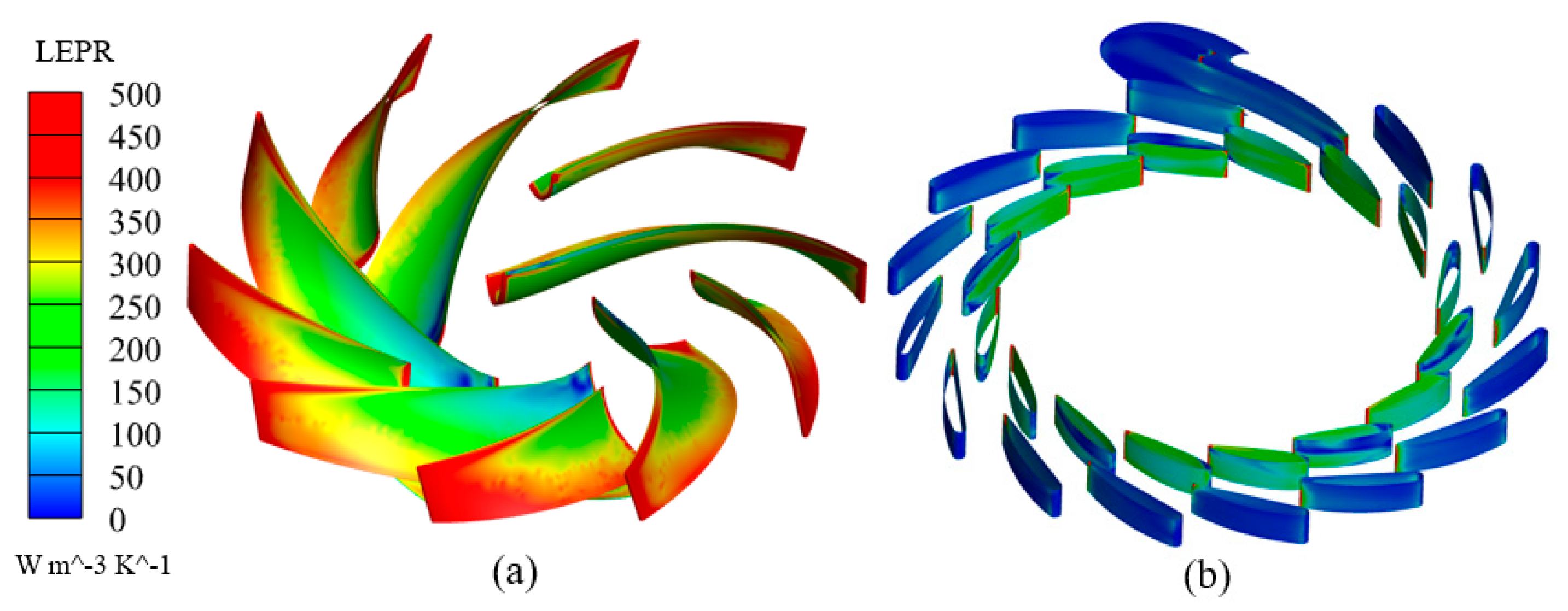
5.4. LEPR Distribution on the Wall
Since the flow within the pump–turbine is a viscous incompressible fluid, the viscous dissipation of the flow with the walls of the components during the flow process becomes part of the energy loss. When the fluid flows through the pump–turbine, it interacts with the guide vanes and runner blades, and its wall entropy production accounts for the largest proportion of the wall loss of the whole flow path; therefore, this study only investigated and analyzed the wall entropy production of the movable guide vanes and runner blades, and the results are shown in Figure 13. It was found that the wall entropy production at the blades in Figure 13a was mainly concentrated near the inlet of the leading edge of the blades and the pressure surface side of the trailing edge outlet, which is due to the large speed of rotation compared to the flow rate, resulting in energy loss due to the large shock loss generated after the fluid impacts the rotor blades. Meanwhile, the wall entropy production at the guide/stay vanes was mainly concentrated at the leading edge of the vanes and the pressure side of the vanes, and there was no high-entropy production region at the trailing edge (Figure 13b). This is due to the fact that when the fluid is spun out of the runner, it hits the pressure surface of the guide vanes again, and at the suction side and trailing edge of the vanes, and decoupling occurs, resulting in less energy loss as no fluid passes at the wall.
6. Conclusions
In this paper, for the hump characteristic and hysteresis effect of a splitter blade pump–turbine, based on the entropy production theory and entropy wall function theory, through numerical simulation, combined with the internal flow, the distribution of entropy production and the hydraulic loss of the high-, medium- and low-flow conditions in the direction of increasing flow rate and decreasing flow rate were investigated. The main conclusions of the study are as follows:
- As with the traditional pump–turbine, the pump–turbine with diverter vanes also has hump characteristics and hysteresis effects in the pumping condition.
- The hydraulic losses of the runner are mainly distributed in the leading and trailing edges of the long blades and the suction surface area, while the energy loss near the short blades is very low. This is mainly due to the energy loss caused by the high velocity gradient at the wall surface and the resulting flow disturbance.
- Compared with the traditional runner [40], the pumping condition of the vortex of the impeller in the pump–turbine with the splitter blade in was significantly reduced. It was found that in the pumping condition, the hydraulic loss at the outlet of the runner was concentrated in the vicinity of the trailing edge of the long blades, whereas there was no such phenomenon in the case of the short blades. This indicates that the use of a combination of splitter blades contributes to the energy performance of the pump–turbine.
In summary, the pump–turbine with splitter vane also has a hump characteristic and hysteresis effect in pumping conditions. On the other hand, the hysteresis phenomenon is caused by the difference in the distribution and intensity of unsteady flow patterns in the two flow directions. This depends on the working conditions. This will provide a relevant reference for the stable operation of pump–turbines and the design of safety margins in the future.
Author Contributions
Conceptualization, R.S.; methodology, X.Z.; formal analysis, R.S.; resources, Z.L. and T.G.; data curation, L.D.; writing—original draft, G.D.; supervision, Z.L.; funding acquisition, Z.L. and T.G. All authors have read and agreed to the published version of the manuscript.
Funding
This work was financially supported by the National Natural Science Foundation of China (NSFC) (Grant Nos. 52069010; 52369017) and the Ranking of the top of the list for science and technology projects of Yunnan Province (No.: 202204BW050001).
Data Availability Statement
Some or all data, models, or codes that support the findings of this study are available from the corresponding author upon reasonable request.
Acknowledgments
I would like to thank Zhimei Luo for his guidance during the research process, Deyou Li for answering my questions, and my fellow students for helping me with my studies.
Conflicts of Interest
The authors declare no conflict of interest.
Nomenclature
| H | head of pump–turbine [m] |
| Q | discharge [m3·s−1] |
| GVO | guide vane opening [mm] |
| EnD | energy factor |
| TnD | torque factor |
| QnD | discharge factor |
| T | temperature [K] |
| ρ | density [kg/m3] |
| u | velocity [m·s−1] |
| Fx | body force [N] |
| μ | hydrodynamic viscosity [Pa·s] |
| entropy production rate of time-averaged movement [kW m−3 K−1] | |
| entropy production rate of velocity fluctuation [kW m−3 K−1] | |
| β | Constant = 0.09 |
| μeff | effective dynamic viscosity [kg m−1 s−1] |
| μt | turbulent dynamic viscosity [kg m−1 s−1] |
| ε | turbulent dissipation rate [m2·s−3] |
| ω | turbulent eddy frequency [s−1] |
| k | turbulent energy [m2/s2] |
| y+ | Dimensionless distance |
| η | efficiency [%] |
| γ | relative error [%] |
| δij | Crowe dick symbol |
| Dec | the direction of decreasing discharge |
| Inc | the direction of increasing discharge |
| BEP | best efficiency point |
| h∆P | Head loss computed by differential pressure method |
| hpro | Head loss computed by entropy production method |
References
- Feng, C. Study on System Identification and Control Law under Complex Conditions of Pumped Law under Complex Conditions of Pumped. Ph.D. Thesis, Huazhong University of Science & Technology, Wuhan, China, May 2020. [Google Scholar]
- Lu, G.C. Investigations on the Influence of the Flow Separation in Guide Vane Channels on the Positive Slope on the Pump Performance Curve in a Pump-Turbine. Ph.D. Thesis, Tsinghua University, Beijing, China, June 2018. [Google Scholar]
- Jese, U.; Fortes-Patella, R.; Dular, M. Numerical study of Pump-turbine instabilities under pumping mode off-design conditions. In Proceedings of the ASME-JSME-KSME Joint Fluids Engineering Conference, Seoul, Republic of Korea, 26–31 July 2015. [Google Scholar] [CrossRef]
- Yang, J.; Pavesi, G.; Yuan, S.; Cavazzini, G.; Ardizzon, G. Experimental Characterization of a Pump-Turbine in Pump Mode at Hump Instability Region. J. Fluids Eng.-Trans. ASME 2015, 137, 051109. [Google Scholar] [CrossRef]
- Li, D.Y.; Han, L.; Wang, H.; Gong, R.; Wei, X.; Qin, D. Flow characteristics prediction in pump mode of a pump turbine using large eddy simulation. Proc. Inst. Mech. Eng. Part E J. Process Mech. Eng. 2017, 231, 961–977. [Google Scholar] [CrossRef]
- Braun, O.; Kueny, J.L.; Avellan, F. Numerical analysis of flow phenomena related to the unstable energy-discharge characteristic of a pump-turbine in pump mode. In Proceedings of the ASME Fluids Engineering Division Summer Conference, Houston, TX, USA, 19–23 June 2005; pp. 1075–1080. [Google Scholar] [CrossRef]
- Liu, J.; Liu, S.; Wu, Y.; Jiao, L.; Wang, L.; Sun, Y. Numerical investigation of the hump characteristic of a pump–turbine based on an improved cavitation model. Comput. Fluids 2012, 68, 105–111. [Google Scholar] [CrossRef]
- Lu, G.; Zuo, Z.; Sun, Y.; Liu, D.; Tsujimoto, Y.; Liu, S. Experimental evidence of cavitation influences on the positive slope on the pump performance curve of a low specific speed model pump-turbine. Renew. Energy 2017, 113, 1539–1550. [Google Scholar] [CrossRef]
- Li, D.; Zhu, Y.; Lin, S.; Gong, R.; Wang, H.; Luo, X. Cavitation effects on pressure fluctuation in pump-turbine hump region. J. Energy Storage 2022, 47, 103936. [Google Scholar] [CrossRef]
- Li, Q.; Wang, Y.; Liu, C.; Han, W. Study on Unsteady internal flow characteristics in hump zone of mixed flow pump turbine. J. Gansu Sci. 2017, 29, 54–58. [Google Scholar] [CrossRef]
- Qin, Y.L. Investigation on the Influence of Geometric Factors at Runner Outlet on the Hump Characteristics of a Pump-Turbine. Master’s Thesis, Harbin Institute of Technology, Harbin, China, June 2020. [Google Scholar] [CrossRef]
- Ciocan, G.; Desvignes, V.; Combes, J.; Parkinson, E.; Kueny, J. Experimental and numerical unsteady analysis of rotor-stator interaction in a pump-turbine. In Proceedings of the XIX IAHR International Symposium on Hydraulic Machinery and Cavitation, Singapore, 9–11 September 1998; pp. 210–219. [Google Scholar]
- Li, X.; Zhu, Z.; Li, Y.; Chen, X. Experimental and numerical investigations of head-flow curve instability of a single-stage centrifugal pump with volute casing. Proc. Inst. Mech. Eng. Part A J. Power Energy 2016, 230, 633–647. [Google Scholar] [CrossRef]
- Xiao, Y.; Yao, Y.; Wang, Z.; Zhang, J.; Luo, Y.; Zeng, C.; Zhu, W. Hydrodynamic mechanism analysis of the pump hump district for a pump-turbine. Eng. Comput. 2016, 33, 957–976. [Google Scholar] [CrossRef]
- Ye, W.X.; Ikuta, A.; Chen, Y.N.; Miyagawa, K.; Luo, X.W. Numerical simulation on role of the rotating stall on the hump characteristic in a mixed flow pump using modified partially averaged Navier-Stokes model. Renew. Energy 2020, 166, 91–107. [Google Scholar] [CrossRef]
- Ran, H.J.; Zhang, Y.; Luo, X.W.; Xu, H. Numerical simulation of the positive-slope performance curve of a reversible hydro-turbine in pumping mode. J. Hydroelectr. Eng. 2011, 30, 175–179. [Google Scholar] [CrossRef]
- Guedes, A.; Kueny, J.L.; Ciocan, G.D.; Avellan, F. Unsteady Rotor-Stator Analysis of A Hydraulic Pump-Turbine—CFD and Experimental Approach. In Proceedings of the 21st IAHR Symposium on Hydraulic Machinery and Systems, Lausanne, Switzerland, 9–12 September 2002. [Google Scholar]
- Shibata, A.; Hiramatsu, H.; Komaki, S.; Miyagawa, K.; Maeda, M.; Kamei, S.; Hazama, R.; Sano, T.; Iino, M. Study of flow instability in off design operation of a multistage centrifugal pump. J. Mech. Sci. Technol. 2016, 30, 493–498. [Google Scholar] [CrossRef]
- Wang, L.Q.; Liu, J.T.; Zhang, L.F.; Qin, D.Q.; Jiao, L. Low flow s fluctuation characteristics in pump-turbine s pump mode. J. Zhejiang Univ. Eng. Sci. 2011, 45, 1239–1243. [Google Scholar] [CrossRef]
- Sun, Y.K. Instability Characteristics and Instability Characteristics and Pump Performance Curves of a Low-Specific-Speed Pump-Turbine. Ph.D. Thesis, Tsinghua University, Beijing, China, May 2016. [Google Scholar]
- Chen, J.X. Experimental Investigation of Hysteresis Characteristics in the Hump and S-Shaped Region of a Pump-Turbine. Master’s Thesis, Harbin Institute of Technology, Harbin, China, September 2017. [Google Scholar]
- Li, D.Y.; Chang, H.; Zuo, Z.G.; Wang, H.J.; Li, Z.G.; Wei, X.Z. Experimental investigation of hysteresis on pump performance characteristics of a model pump-turbine with different guide vane openings. Renew. Energy 2020, 149, 652–663. [Google Scholar] [CrossRef]
- Li, D.Y.; Wang, H.J.; Chen, J.X.; Nielsen, T.K.; Qin, D.Q. Hysteresis Characteristic in the Hump Region of a Pump-Turbine Model. Energies 2016, 9, 620. [Google Scholar] [CrossRef]
- Li, D.Y.; Wang, H.J.; Qin, Y.L.; Han, L.; Wei, X.Z.; Qin, D.Q. Entropy production analysis of hysteresis characteristic of a pump-turbine model. Energy Convers. Manag. 2017, 149, 175–191. [Google Scholar] [CrossRef]
- Li, D.Y.; Gong, R.Z.; Wang, H.J.; Fu, W.W.; Wei, X.Z.; Liu, Z.S. Fluid flow analysis of drooping phenomena in pump mode for a given guide vane setting of a pump-turbine model. J. Zhejiang Univ. Sci. A 2015, 16, 851–863. [Google Scholar] [CrossRef]
- Tao, R.; Xiao, R.F.; Yang, W.; Liu, W.C. Hump characteristic of reversible pump-turbine in pump mode. J. Drain. Irrig. Mach. Eng. 2014, 32, 936. [Google Scholar] [CrossRef]
- Kock, F.; Herwig, H. Local entropy production in turbulent shear flows: A high-Reynolds number model with wall functions. Int. J. Heat Mass Transf. 2004, 7, 2205–2215. [Google Scholar] [CrossRef]
- Li, D.Y.; Gong, R.Z.; Wang, H.J.; Xiang, G.M.; Wei, X.Z.; Qin, D.Q. Entropy production analysis for hump characteristics of a pump turbine model. Chin. J. Mech. Eng. 2016, 29, 803–812. [Google Scholar] [CrossRef]
- Lu, J.L.; Wang, L.K.; Liao, W.L.; Zhao, Y.P.; Ji, Q.F. Entropy production analysis for vortex rope of a turbine model. J. Hydraul. Eng. 2019, 50, 233–241. [Google Scholar] [CrossRef]
- Zeng, H.J.; Li, Z.G.; Li, D.Y.; Li, Q.F. Relationship between flow pulsation and entropy production rate of pump turbine. J. Drain. Irrig. Mach. Eng. 2022, 40, 777–784. [Google Scholar]
- Li, D.Y. Investigation on Flow Mechanism and Transient Characteristics in Hump Region of A Pump-Turbine. Ph.D, Thesis, Harbin Institute of Technology, Harbin, China, June 2017. [Google Scholar]
- Li, D.K.; Gui, Z.H.; Yan, X.T.; Zheng, Y.; Kan, K. Hydraulic loss distribution of pump-turbine operated in pump mode based on entropy production method. South North Water Transf. Water Sci. Technol. 2023, 21, 390–397. [Google Scholar]
- Chen, H.Y. Application of Long-and Short-Blade Runner in Qingyuan Pumped Storage Power Station. Mech. Electr. Tech. Hydropower Stn. 2016, 39, 5–8. [Google Scholar] [CrossRef]
- Du, R.X.; Wang, Q.; Enomoto, Y.; Chen, H.Y. Application of Splitter Blades Runner Pump Turbine in Qingyuan Pump Storage Station. Hydropower Pumped Storage 2016, 2, 39–44. [Google Scholar] [CrossRef]
- Mathieu, J.; Scott, J. An Introduction to Turbulent Flow; Cambridge University Press: Cambridge, UK, 2000. [Google Scholar]
- Herwig, H.; Kock, F. Direct and indirect methods of calculating entropy generation rates in turbulent convective heat transfer problems. Heat Mass Transf. 2007, 43, 207–215. [Google Scholar] [CrossRef]
- Melzer, S.; Pesch, A.; Schepeler, S.; Kalkkuhl, T.; Skoda, R. Three-Dimensional Simulation of Highly Unsteady and Isothermal Flow in Centrifugal Pumps for the Local Loss Analysis Including a Wall Function for Entropy Production. J. Fluids Eng.-Trans. ASME 2020, 142, 111209. [Google Scholar] [CrossRef]
- Li, D.; Wang, H. Numerical simulation of hysteresis characteristic in the hump region of a pump-turbine model. Renew. Energy 2018, 115, 433–447. [Google Scholar] [CrossRef]
- Li, Z.; Liu, X.; Xu, L. A Review of Research on Hump Characteristics of High-head Pump-turbine. Hydropower Pumped Storage 2023, 9, 39–47. [Google Scholar] [CrossRef]
- Li, D.; Zuo, Z.; Wang, H.; Liu, S.; Wei, X.; Qin, D. Review of positive slopes on pump performance characteristics of pump-turbines. Renew. Sustain. Energy Rev. 2019, 112, 901–916. [Google Scholar] [CrossRef]
Figure 1.
Characteristic curve of flow head.

Figure 2.
Computational domain of pump–turbine model.

Figure 3.
Detailed of the pump–turbine grid (Red arrow represents the detailed presentation of the mesh).
Figure 3.
Detailed of the pump–turbine grid (Red arrow represents the detailed presentation of the mesh).
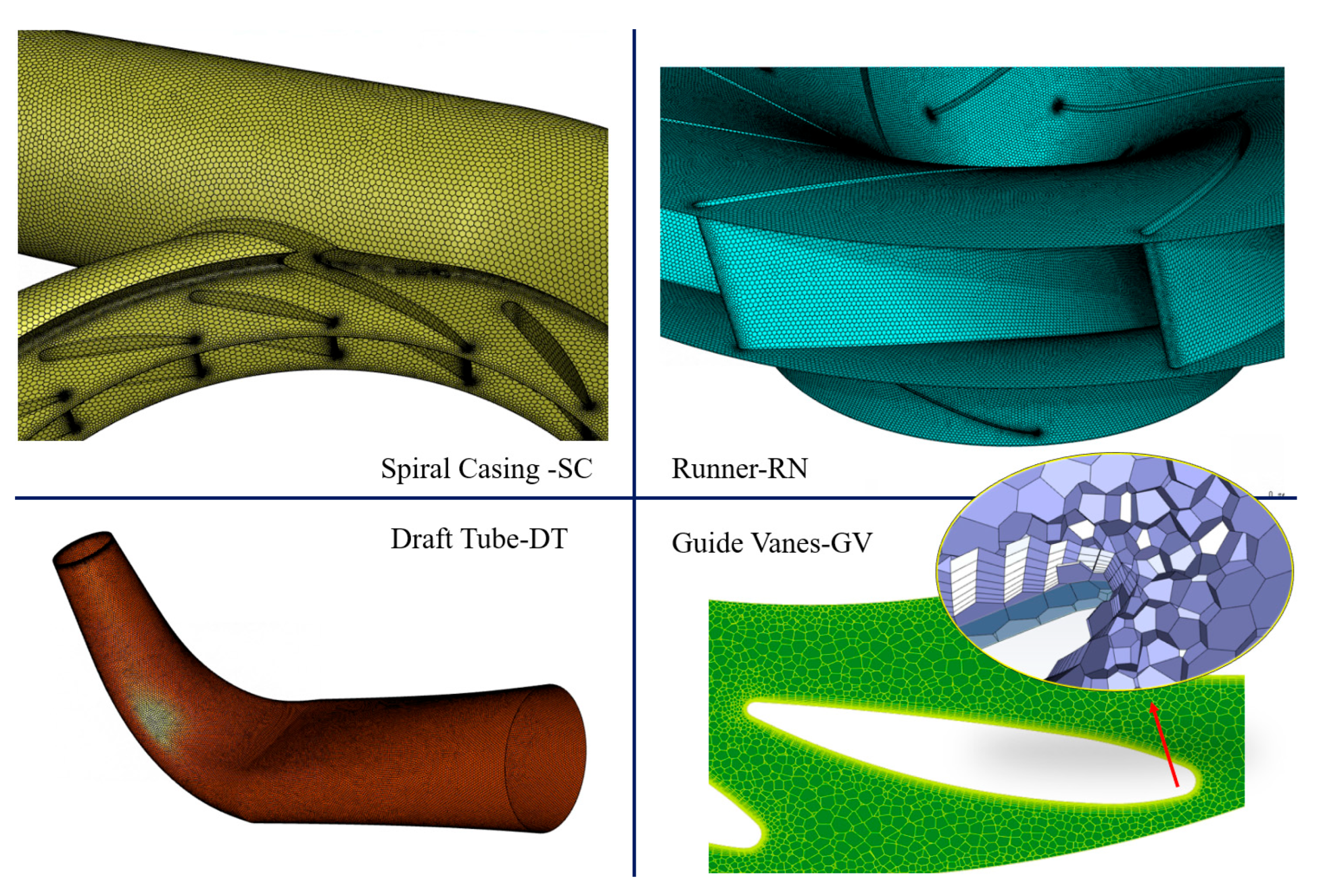
Figure 4.
Validation of grid independence.

Figure 5.
Flow-head curve for pump condition at 23 mm GVO.

Figure 6.
Comparison between head loss calculated using the two methods in the direction of increasing discharge.
Figure 6.
Comparison between head loss calculated using the two methods in the direction of increasing discharge.
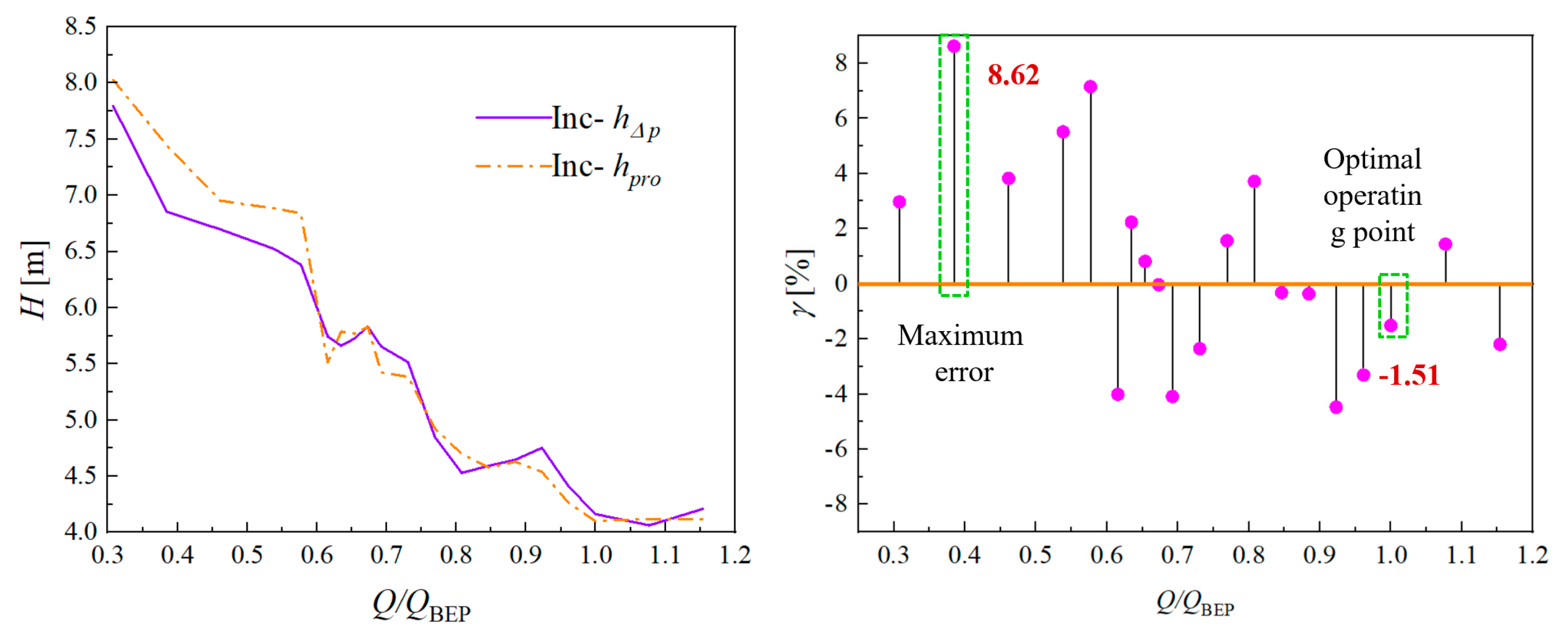
Figure 7.
Comparison between head loss calculated using the two methods in the direction of decreasing discharge.
Figure 7.
Comparison between head loss calculated using the two methods in the direction of decreasing discharge.

Figure 8.
Entropy production distribution.

Figure 9.
Entropy production distribution for different parts. (a) Direction of flow increase; (b) direction of flow decrease.
Figure 9.
Entropy production distribution for different parts. (a) Direction of flow increase; (b) direction of flow decrease.
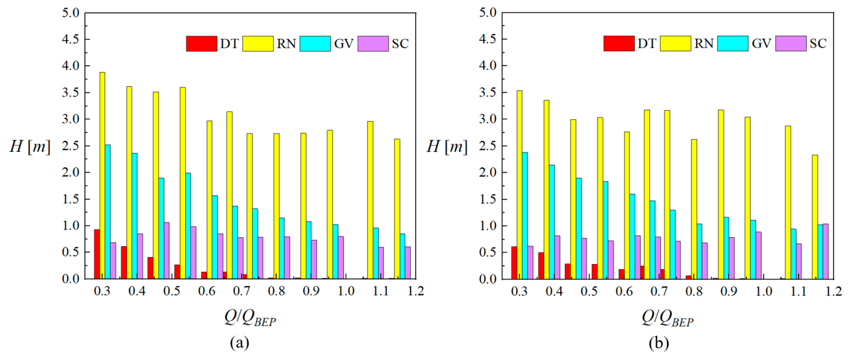
Figure 10.
LEPR distribution in the runner. (a) the LEPR distribution of 1.15 QBEP. (b) the LEPR distribution of 1.0 QBEP. (c) the LEPR distribution of 0.81 QBEP. (d) the LEPR distribution of 0.73 QBEP. (e) the LEPR distribution of 0.63 QBEP. (f) the LEPR distribution of 0.38 QBEP.
Figure 10.
LEPR distribution in the runner. (a) the LEPR distribution of 1.15 QBEP. (b) the LEPR distribution of 1.0 QBEP. (c) the LEPR distribution of 0.81 QBEP. (d) the LEPR distribution of 0.73 QBEP. (e) the LEPR distribution of 0.63 QBEP. (f) the LEPR distribution of 0.38 QBEP.
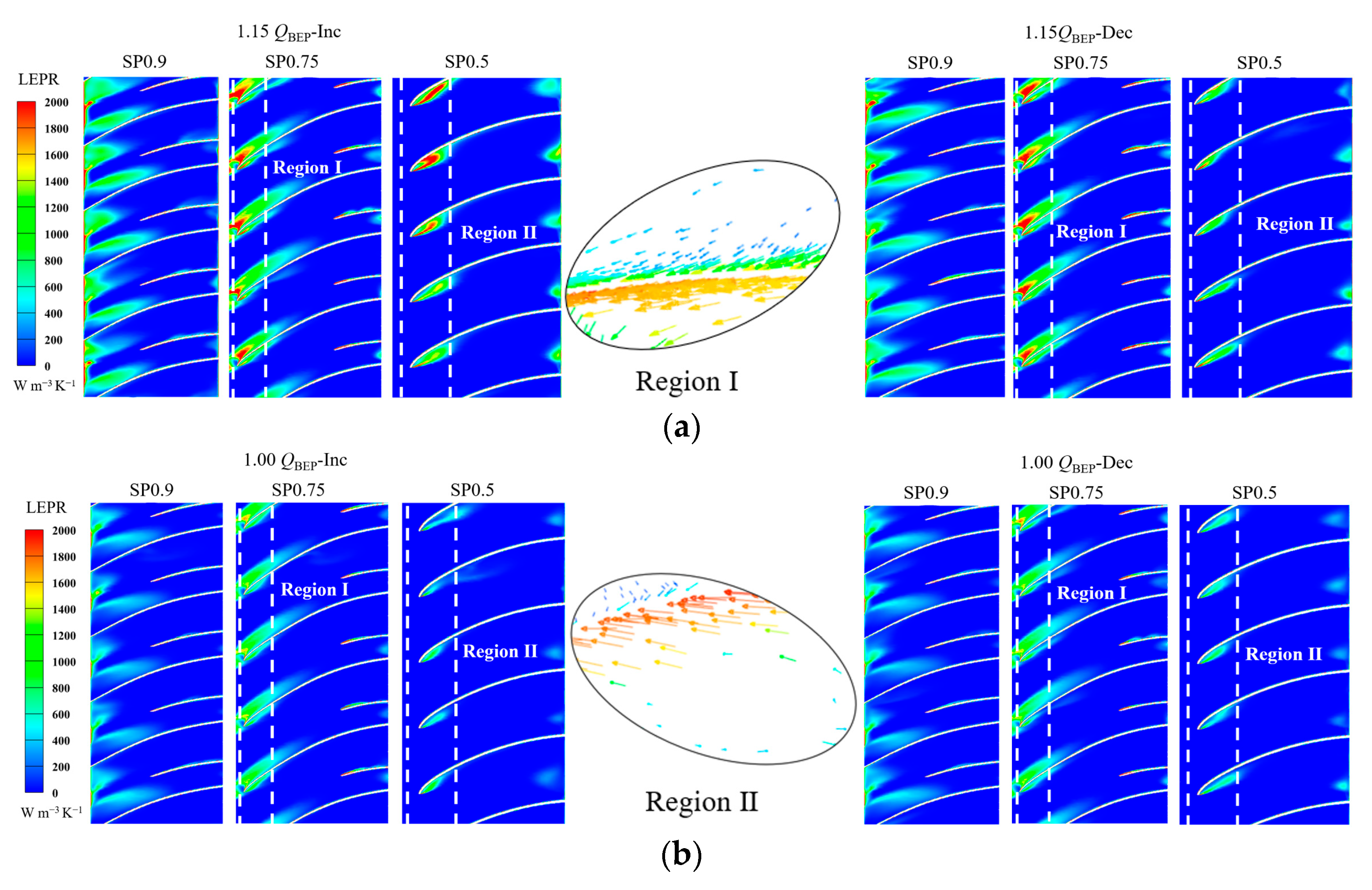

Figure 11.
LEPR distribution in the guide/stay vanes. (a) the LEPR distribution of 1.15 QBEP. (b) the LEPR distribution of 1.0 QBEP. (c) the LEPR distribution of 0.81 QBEP. (d) the LEPR distribution of 0.73 QBEP. (e) the LEPR distribution of 0.63 QBEP. (f) the LEPR distribution of 0.38 QBEP.
Figure 11.
LEPR distribution in the guide/stay vanes. (a) the LEPR distribution of 1.15 QBEP. (b) the LEPR distribution of 1.0 QBEP. (c) the LEPR distribution of 0.81 QBEP. (d) the LEPR distribution of 0.73 QBEP. (e) the LEPR distribution of 0.63 QBEP. (f) the LEPR distribution of 0.38 QBEP.


Figure 12.
Distribution of entropy production in each cross-section of straight conical section of draft tube in different working conditions.
Figure 12.
Distribution of entropy production in each cross-section of straight conical section of draft tube in different working conditions.

Figure 13.
Entropy production of splitter blades (a) and guide/stay vane wall (b).

Table 1.
Parameters of the pump–turbine.
| Parameter | Symbol | Value |
|---|---|---|
| Specific speed | nq | 31.633 |
| Runner blade number (long) | Zr1 | 5 |
| Runner blade number (short) | Zr2 | 5 |
| Guide vane number | Zg | 16 |
| Stay vane number | Zs | 16 |
| Runner outlet | D1m | 540.5 mm |
| Runner inlet | D2m | 287.5 mm |
| Guide vane height | B0 | 52 mm |
Table 2.
Details of grids.
| Component | Case1 | Case2 | Case3 |
|---|---|---|---|
| Draft tube | 499,451 | 931,463 | 1,107,572 |
| Runner | 2,576,221 | 3,636,685 | 5,997,393 |
| Guide vane | 887,352 | 1,357,038 | 1,840,524 |
| Stay vane and volute | 1,874,117 | 2,372,530 | 2,563,200 |
| Total | 5,837,141 | 8,297,716 | 11,508,689 |
Disclaimer/Publisher’s Note: The statements, opinions and data contained in all publications are solely those of the individual author(s) and contributor(s) and not of MDPI and/or the editor(s). MDPI and/or the editor(s) disclaim responsibility for any injury to people or property resulting from any ideas, methods, instructions or products referred to in the content. |
© 2024 by the authors. Licensee MDPI, Basel, Switzerland. This article is an open access article distributed under the terms and conditions of the Creative Commons Attribution (CC BY) license (https://creativecommons.org/licenses/by/4.0/).
Share and Cite
MDPI and ACS Style
Dong, G.; Luo, Z.; Guo, T.; Zhang, X.; Shan, R.; Dai, L. The Splitter Blade Pump–Turbine in Pump Mode: The Hump Characteristic and Hysteresis Effect Flow Mechanism. Processes 2024, 12, 324. https://doi.org/10.3390/pr12020324
AMA Style
Dong G, Luo Z, Guo T, Zhang X, Shan R, Dai L. The Splitter Blade Pump–Turbine in Pump Mode: The Hump Characteristic and Hysteresis Effect Flow Mechanism. Processes. 2024; 12(2):324. https://doi.org/10.3390/pr12020324
Chicago/Turabian StyleDong, Guanghe, Zhumei Luo, Tao Guo, Xiaoxu Zhang, Rong Shan, and Linsheng Dai. 2024. "The Splitter Blade Pump–Turbine in Pump Mode: The Hump Characteristic and Hysteresis Effect Flow Mechanism" Processes 12, no. 2: 324. https://doi.org/10.3390/pr12020324
Note that from the first issue of 2016, this journal uses article numbers instead of page numbers. See further details here.