
Benefits and Limitations of Artificial Neural Networks in Process Chromatography Design and Operation
Institute for Separation and Process Technology, Clausthal University of Technology, Leibnizstraße 15, D-38678 Clausthal-Zellerfeld, Germany
*
Author to whom correspondence should be addressed.
Processes 2023, 11(4), 1115; https://doi.org/10.3390/pr11041115
Submission received: 7 March 2023
/
Revised: 29 March 2023
/
Accepted: 3 April 2023
/
Published: 5 April 2023
(This article belongs to the Special Issue Towards Autonomous Operation of Biologics and Botanicals)
Abstract
:Due to the progressive digitalization of the industry, more and more data is available not only as digitally stored data but also as online data via standardized interfaces. This not only leads to further improvements in process modeling through more data but also opens up the possibility of linking process models with online data of the process plants. As a result, digital representations of the processes emerge, which are called Digital Twins. To further improve these Digital Twins, process models in general, and the challenging process design and development task itself, the new data availability is paired with recent advancements in the field of machine learning. This paper presents a case study of an ANN for the parameter estimation of a Steric Mass Action (SMA)-based mixed-mode chromatography model. The results are used to exemplify, discuss, and point out the effort/benefit balance of ANN. To set the results in a wider context, the results and use cases of other working groups are also considered by categorizing them and providing background information to further discuss the benefits, effort, and limitations of ANNs in the field of chromatography.
1. Introduction
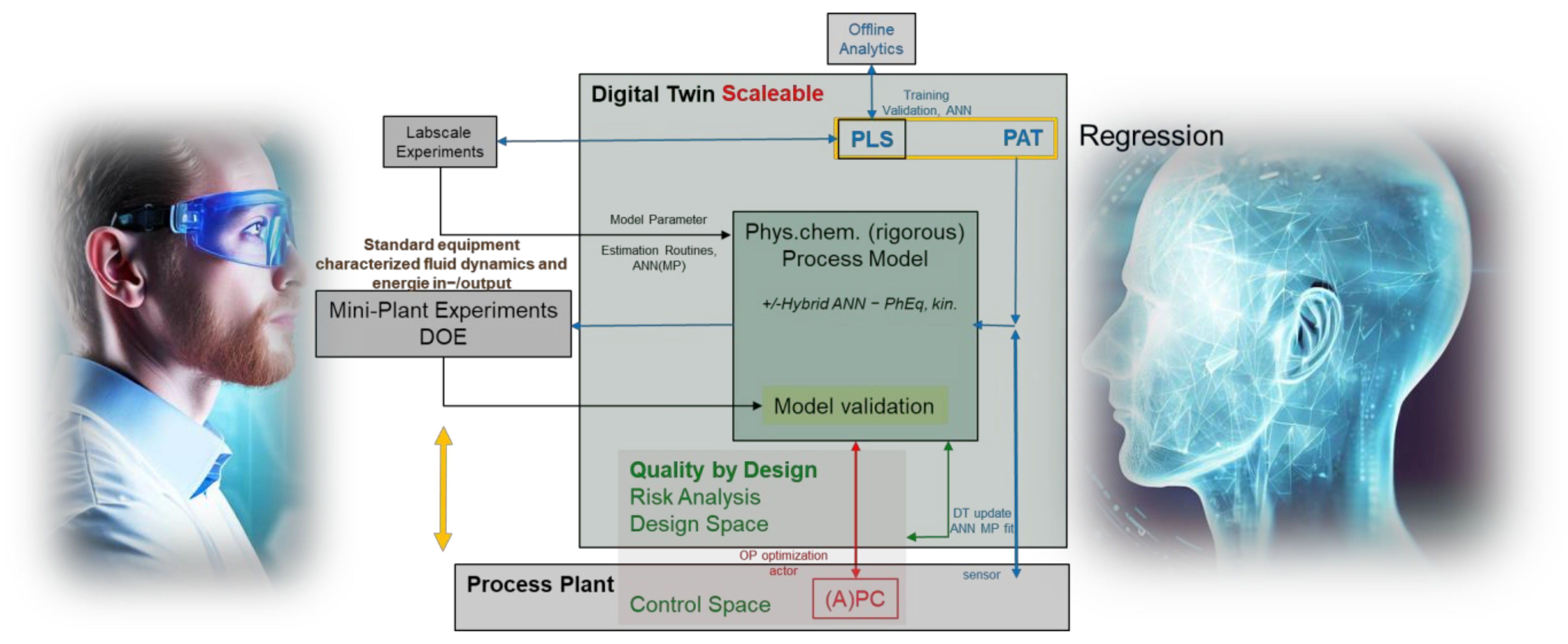
With the ongoing digitalization of the industry, the so-called Industry 4.0, previously inaccessible or barely accessible data are now available. Previously handwritten or printed process data is digitalized or accessible via standardized interfaces like OPC UA [1,2,3]. This digitalization also enables new opportunities in process development and optimization [3,4]. One concept is the implementation of Digital Twins of the process. These digital twins are digital copies of the process [5,6]. In the context of process engineering, these are sophisticated models of the processes, as shown in Figure 1. These do not only support process development in the early stages but also enable the tracking of the process itself and its deviations. This can be utilized to predict consequences and improve process performance and/or quality [7,8].
Digital twins need to be scalable to be useful in process development, manufacturing, and piloting. However, certain aspects, such as phase equilibrium behavior and mass transfer kinetics, do not change with scale, while others, like fluid dynamics and energy distribution, do. To create a predictive process model, it is important to separate these effects and determine the model parameters at the laboratory scale. Then only the fluid dynamics have to be changed at larger scales. In order to rely on any model-based decisions, these models must be validated experimentally with accuracy and precision. Such model validation is distinctly based on a statistical design of experiments (DoE) plan at mini plants. The scalable digital twin concept is shown in Figure 1 [9]. Artificial neural networks (ANN) can be used in a number of ways. They can serve as regressors for process analytical technology (PAT) sensor data or replace methods like the partial least squares (PLS) algorithm. ANN can also be used to determine model parameters instead of minimizing the sum of least square errors between experimental and simulated datasets. Additionally, ANNs can be used to adapt the digital twin’s process and model parameters to real-time operation data. Another application of ANN is in process models or as part of such models, e.g., hybrid models. A complete framework for total process design and operation has already been established [10,11,13].
Concerning process chromatography, over the years, many methods for modeling and optimization of process chromatography have been suggested and implemented [14,15,16,17,18,19,20]. Instead of only exploiting existing methods, new methods like the utilization of machine learning algorithms are explored. These range from common data analysis tools like the Partial Least Squares (PLS) algorithm to the utilization of artificial neural networks (ANN) [21,22,23,24], which are considered universal approximators [25].
For the sake of simplicity, this work focuses on artificial neural networks (ANNs). The ANNs can be utilized in all levels of Figure 2. In the context of process chromatography, current ANN approaches can be simplified into the following categories (Figure 3). Depending on the category, different types of solutions can be realized. On the other hand, different types of training and different perquisites and amounts of data samples are necessary for a successful implementation.
Figure 3a describes a general regressor, which is a type of ANN that maps inputs to outputs without considering any underlying mechanistic relationships. This type of ANN works best within its training area and may not be able to extrapolate data beyond its limits. The outputs are produced in a fraction of seconds [26,27,28,29,30,31,32,33,34,35].
Figure 3b describes an ANN that is still a general regressor but tries to identify model parameters from measurements. In this case, the ANN supplies parameters to the model. It is necessary to consider the model input, which affects the input of the ANN, in the training dataset. The outputs are also produced in fractions of a second [22,36,37,38,39,40,41].
Figure 3c describes an ANN that is part of the equation system of the model. The ANN receives input from the equation system and delivers results back to the equation system. In this case, the ANN is a function that can adapt to the problem, meaning it learns to be the missing equation(s) of the mechanistic model based on supported data. In other words, in the classical approach, only parameters of a function are adjusted to match the data, while in this approach, an entire function is evolved to match the reference data. Therefore, this is called a hybrid model in the context of this paper because the model itself consists of data-driven and mechanistic elements. In this scenario, the output of the model is primarily constrained in terms of speed and accuracy by the limitations of the equation system and the information contained within the available data [23,42,43].
Figure 3d depicts a so-called physics-informed neural network (PINN) that constitutes the model, or at least a significant portion of it. In this scenario, the ANN learns the underlying mechanistic equations, ranging from algebraic equations to partial differential equations, and can account for any unknown effects through the data supplied. The model output is generated quickly, within a fraction of a second, making it a valuable tool for real-time applications. This type is still in an early stage of research in the field of chromatography [44,45,46]. Further information about PINNS can be found in [47,48,49].
Before discussing the benefits and drawbacks of each approach, it is important to understand how the training in each of the approaches works in general. This is also essential for a better understanding of the effort and opportunities ANN offers. A simplified scheme is shown in Figure 4. During training, the ANN receives an input and a desired output. The current result is then compared to the desired result, and the error is calculated based on a user-defined formula. The training algorithm then tries to minimize this error by adjusting the ANN parameters accordingly via backpropagation [50,51]. This process is repeated until there is no more improvement over a specified number of training epochs or a certain threshold is met. To avoid overfitting or underfitting, several approaches are taken. At first, an ANN architecture has to be developed that is able to perform the mapping from inputs to outputs of the given data without overfitting. This is mostly influenced by the underlying complexity of the information in the data itself [50,51]. In practice, different amounts of layers and neurons and different activation functions are tested until a promising candidate emerges [31,37,44,52]. In chromatography, these architectures mostly follow the fully connected feed-forward scheme. Further performance-enhancing options are different loss functions and different training algorithms with different parameters. Additionally, techniques such as dropout or regularization are utilized to increase the generalization ability of ANNs. Thereby, generalization means the error of the ANN on unseen data [50,51]. This generalization ability is also greatly influenced by the amount of training data, as shown by Pirrung et al. [31]. In the end, the optimization of all those so-called hyperparameters leads to multiple networks being trained and evaluated during the whole ANN development process. Detailed information concerning ANNs in general and the training process can be found in Fausett [50] and Goodfellow at el. [51].
Figure 4a shows the case of the Figure 3a category regressor and the Figure 3b category regressor with the subsequent model. Information exists only in the data. In this case, an appropriate amount of data is required for training, and the training duration mainly depends on the network architecture and the amount and complexity of the data. This type of model may not be predictive outside the bounds of the training data. An example is a regressor for isotherm parameters or retention time.
Figure 4b shows the simplified training scheme of a physics-informed neural network (PINN) from Figure 3c. To train a PINN, physical principles are first formulated as mathematical equations, which are then incorporated into the loss function used in the training process. The physical constraints can range from simple algebraic equations to complex partial differential equations (PDE). The neural network then tries to optimize the loss function by minimizing the error between predicted and actual outcomes while satisfying the imposed physical constraints. The error can be calculated by using automatic differentiation [47,48,49], thus no human interaction is necessary. By doing so, the network learns the underlying physical principles governing the system being studied, leading to more accurate and reliable predictions. This type of model is predictive because it follows the rules of the underlying PDEs. On the other hand, the model has to be retrained if the initial conditions or boundary conditions are changed, as stated by Subraveti et al. [46].
Figure 4c shows most of the information is in the model equation system, and the missing information (e.g., the isotherm) is in the data. In this case, the ANN is part of the equation system, and the data is only needed for the non-mathematically described part of the model. The whole model has to be solved for each ANN training epoch, and the training is limited by the complexity of the missing data and the model itself [23,42,43]. This hybrid model learns the behavior that is not described in the model equation, and the ANN is modified so that the whole model fits the data. This is a form of fitting, but instead of modifying parameters, a whole function is modified. The model is only predictive within the range of the input data [23].
Most examples of ANNs as regressors, as shown in Figure 3a, are used for process optimization. First, an ANN is developed to predict certain values. Then a standard optimization algorithm is used to perform the optimization with the ANN’s inputs and outputs. Examples are Golubović et al. [28], Nagrath et al. [30], and Pirrung et al. [31].
Golubović et al. [28] used ANNs for retention factor optimization of mycophenolate mofetil (MFM) and its degradation products. The ANN predicted the retention factors based on buffer composition, flow rate, and column temperature. A purely experimental dataset of 33 samples based on the Central Composite Design (CCD) was used, which is able to detect linear and quadratic effects. The ANN outperformed standard Multilinear Regression (MLR) and enabled the reduction of the experiment duration from 6.2 min to 5.2 min. The drawbacks of this approach may be the limitations on the area and information of the CCD design space and the experimental effort. Designing and performing these experiments on a preparative chromatography scale may also not be possible. On the other hand, no process knowledge or process modeling is necessary for this approach. Even no ANN knowledge is necessary, as the network was optimized by trial and error.
Nagrath et al. [30] used, in contrast to Golubović et al. [28], simulated data instead of experimental data to overcome the experimental bottleneck, which becomes more relevant the more complex the task becomes. As stated by Nagrath et al. [30], a rising number of parameters has become a critical issue in optimization procedures solely based on mechanistic models as proposed by Narayanan et al. [53]. The reasons for that are local minima and the overall computation time. Therefore, the utilization of ANNs for target variable prediction for preparative chromatography optimization is proposed. In this approach for a three-component separation, the gradient slope, flow rate, feed load, and column length were varied in simulations, and their effect on the target variables—production rate, yield, and maximum concentration—was determined to create a training set. In addition, an extra dataset with softer conditions was created to avoid a bias of 0 productivity on the middle component because this overlaps with the left and right components. Additionally, this approach showed good optimization results and greatly benefited from the shorter computation times. On the other hand, prior knowledge is necessary, not only to model the process itself but also to generate suitable data for the ANN training, as shown by the extra dataset for the middle component. In addition, the ANN may be flexible for the trained system, but it has to be completely retrained for new systems and other numbers of components. Therefore, to make an informed decision between the ANN approach and the classical approach, it is crucial to take into account the extra effort needed for data design, generation, and ANN training.
The most complex variant of this approach was performed by Pirrung et al. [31], who utilized ANNs for downstream process optimization. The variable process part consisted of anion exchanger (AEX), cation exchanger (CEX), and hydrophobic interaction (HIC) columns in arbitrary combinations. The maximum number of columns was three. Each column could only be utilized once in a process setup to satisfy the orthogonality principle. The goal was to find an optimal process setup with optimal process parameters without the drawbacks of sequential optimization (suboptimal processes) and the benefits of global parallel process optimization, which yields the possibility of finding the optimal process but also a larger computational effort. Therefore, at first, an ANN-based global optimization was performed, followed by a mechanistic model-based search. The optimization goal was defined as maximizing the yield subject to a purity of greater than 99.9% by manipulating the initial and final salt concentrations and the two cut points for the product pooling and column setup. Similarly, for Nagrath [30], three networks were trained. For each column, a separate ANN with yield and all protein concentrations served as output, while initial and final salt concentrations and the two cut points for the product pooling served as input. The dataset consisted of 1000 samples, but Pirrung et al. showed [31] that the ANN accuracy reached a plateau at dataset sizes of 3000–5000 samples and concluded that a trade-off between accuracy and simulation effort has to be made. The decision for a smaller dataset showed the anticipated worse performance of the ANN global search. This was compensated by the following mechanistic model based on local search. The total optimization time was reduced from 24.7 h to 7.5 h, including dataset generation and ANN training, with a mechanistic model simulation time of 3 s for a single column. Nevertheless, the aforementioned inaccuracies of the ANNs led to an additional evaluation step. Therefore, the authors proposed to always implement a plausibility check. Additionally, accumulating ANN errors may render this method ineffective with an increasing number of neural networks.
Examples for ANNs who act as regressors as depicted in Figure 3b are given by Wang et al. [39,40], Xu et al. [37], and Mouellef et al. [22,36]. In all approaches, the ANNs are used as fast solvers for inverse problems. In other words, they determine mechanistic model parameters from chromatogram simulations of hopefully dedicated experimentally distinct validated models, which is not done in most cases [9]. While Wang et al. [39], Mouellef et al. [22], and Xu et al. [37] only investigated adsorption parameters (Wang: SMA, Mouellef: competitive Langmuir, Xu: competitive Bi-Langmuir), Wang et al. [40] considered maximal loading and salt gradient length in a root cause investigation, and Mouellef et al. [36] considered fluid dynamics and adsorption parameters. However, in later works [22,40], a much smaller parameter area was covered, as only the deviations from a predefined process were to be tracked. On the other hand, references [22,37,39] considered a wide parameter area to realize a parameter estimator for arbitrary three-component mixtures for a fixed column under predefined process conditions. The development procedure of all approaches was nearly the same. Therefore, not every approach is explained in detail. All approaches used simulations for dataset generation. The main reason was the size of the dataset and the associated experimental effort. The used training datasets ranged from 235 [40] simulations to 38,100 simulations [37]. The first step was to design a suitable parameter range based on expert knowledge and sensitivity analysis. Inside that range, the simulations were performed with uniformly distributed parameter variations. After the simulations, the input layer of the ANN had to be designed. A chromatogram itself is a time series of concentrations (or their corresponding UV values) over a range of several minutes to hours, with resolutions that still have to track the peaks’ main characteristics. Accordingly, a single chromatogram consists of a huge number of sample points, with most of its values being constant, as shown in Figure 5.
Thus, Wang et al. [39,40] and Mouellef et al. [22,36] decided to reduce the data amount and complexity by reducing the chromatogram to the necessary information to achieve shorter ANN training durations and reduce the necessary amount of training data, while Xu et al. [37] used the whole chromatogram. Wang et al. [39,40] modified Gauß, fitted the noisy data, normalized it, and cut off all values below 0.2 to reduce the data. Mouellef et al. [22,36] extracted the time points at which certain % values of the maximum peak height were reached and used these as ANN inputs together with the actual peak height. With this approach, different sample rates, which result in different amounts of points in the time series, have not been taken into account (the ANN input structure is fixed after training), while still considering non-ideal peak shapes. The training process itself is similar to other approaches. All groups showed good results and could reduce the parameter determination process to a fraction of a second. On the other hand, Mouellef et al. [22] and Xu et al. [37] showed that the prediction performance shrinks for more complex isotherms (a higher number of parameters), which has to be countered by higher amounts of data. Additionally, the result only works on predefined columns and process conditions, thus limiting its flexibility, especially if column aging is considered. The data generation and ANN training have to be repeated for other amounts of compounds and other conditions. Additionally, the necessary effort for data generation, evaluation, and training may exceed the effort of standard inverse methods, especially if an expert provides good initial values. Therefore, this method may only be beneficial if arbitrary n-component mixtures are to be modeled on exactly the same column.
The only known examples by the authors for Figure 3c, where the ANN is incorporated into the model itself in the area of chromatography, are given by Gao et al. [23] as the first hybrid modeling approach, and Narayanan et al. [43], who follow a comparable path about 10 years later. Both groups used ANNs to model the adsorption behavior on a chromatography resin instead of setting standard isotherm types a priori like Langmuir [54]. Gao [23] used the ANN-based isotherm to replace a flawed Bi-Langmuir isotherm in a Simulated Moving Bed (SMB) enantiomer separation. Narayanan et al. [43] compared different levels of hybridization on a batch capture chromatography step. Both groups showed better results than using the standard isotherm models and stated the methodology as straightforward. In contrast to the aforementioned approaches, the resulting ANN can be used in different process conditions because the ANN-isotherm itself is not influenced by parameters like flow rate or feed concentration, thus rendering it more flexible. Another benefit is the low amount of necessary data compared to the aforementioned approach in Figure 3b. In the end, Gao et al. only utilized one band profile, while Narayanan et al. needed nine data samples. On the other hand, Gao et al. [23] pointed out an obstacle that has to be considered. One is to design experiments that contain enough information for the ANN’s training. They discovered that heavily overloaded peaks worked best. It may be that the ANN needed more information about the asymptotic, i.e., saturation area, of the isotherm. Another obstacle, as pointed out by Narayanan et al. [31], is that the network may attempt to compensate for other deficiencies in the model during training, in addition to the missing isotherm equation. Consequently, while the ANN may produce an isotherm that closely resembles the actual one, there is no guarantee that it will be an exact replica with the exact mechanism, but only an overall fit over the phase equilibrium range chosen.
There are also two currently known authors for physics-informed neural networks (PINNs), as depicted in Figure 3d. Both working groups, Subraveti et al. [44,46] and Santana et al. [45], showed excellent results by replacing the whole chromatography model with PINNs and achieved immense speedups in model computation time, namely in fractions of seconds. Both Santana et al. [45] and Subraveti et al. [46] showed that no experimental data is needed as long as all necessary mechanistic equations are provided. Subraveti et al. [46] also showed that the more complex process setups, like the Pressure Swing Adsorption (PSA), can be modeled and compared using different approaches regarding computation time. Additionally, it was shown by Subraveti et al. in [44] that no implicit or explicit isotherm equations are needed if the PINNs are supported by experimental data. Nevertheless, the prerequisite for this method is sophisticated mechanistic models. As a consequence, PINNs may be ineffective in early model development stages due to the computational effort needed for the training needed after each model adjustment. Because the authors of this paper themselves did not work with PINNs previously, we are hesitant to highlight any further potential problems and benefits as stated by [44,45,46,47,48,49].
An overview of previous publications and their classification in Figure 2 is given in the following Figure 6. Despite promising results, it should be noted that the authors are unaware of any industrial applications utilizing the early publications from Zhao et al. [55] and Gao et al. [23].
The following sections present a case study demonstrating how mixed-mode chromatography model development, as the complex end of chromatography mechanism modeling, could be expedited by the utilization of an ANN. The main goal was to fasten the Steric Mass Action (SMA)-based mixed-mode isotherm parameter determination. The parameter determination via inverse methods proved to be too laborious and time-consuming for non-mixed-mode experts because of the sheer number of parameters and parameters with similar effects on the binding behavior, i.e., seven per component. Therefore, a solution was sought that is both flexible enough to accommodate different substances and applicable to nonprofessionals using machine learning. The solution was the development of an ANN of category Figure 3b, which determines the model parameters from chromatograms and supplies these to the actual model. Until now, no other approach to mixed-mode SMA model parameter determination via machine learning is known to the authors. Because of the expected minimum size of the training dataset, all data was generated via simulations.
2. Materials and Methods
2.1. Chromatography Modeling
The chromatography model has been explained in detail before by Vetter et al. [56] as a modified SMA model for Mixed-Mode based on the Steric Mass Action Isotherm of Nfor et al. [57], which considers the pH and salt concentration changes typical for mixed-mode chromatography (MMC) and the lumped pore diffusion model (LPD) [16]. The mass balance of the two fractions of the mobile phase can be written as Equation (1) [16].
where is the interstitial velocity of the mobile phase, is the axial dispersion coefficient, is the effective transfer coefficient, is the particle diameter, is the porosity, is the concentration in the liquid phase, and is the concentration in the pore. denotes the position in the column of length L and the time. The index denotes the -th component. The boundary conditions are described by Equation (2) for the column inlet and Equation (3) for the column outlet. L depicts the length of the column [16].
The mass transfer coefficient is given by Equation (4). Here, is the film mass transfer coefficient, is the particle radius, and is the pore diffusion coefficient [58]. The pore diffusion coefficient was calculated according to the correlation of Carta [14] and according to Wilson and Geankoplis [59].
The mass balance between the fluid and solid phases for mixed-mode ligands with the same number of each functional group () is given by Equation (5) [57].
where is the loading, is the concentration in the pores, is the stoichiometric coefficient of the salt counterion, and is the stoichiometric coefficient of the hydrophobic ligand with as given in Equation (6) [57].
where is the total number of binding sites, is the charge of the salt counterion, is the molar concentration of salt, is the interaction constant for the IEX part, is the interaction constant for the HIC part, and is the equilibrium constant. Additionally, can be expressed as a function of the pH value and can be written as proposed by Hunt et al. [60] in the linear Equation (7)
The spatial discretization of the partial differential system was done via orthogonal collocation on finite elements. All chromatography simulations were performed on 10 Dell Latatitude E5470 Systems, which were managed by a Dell Precision 3630 System in a client-server setup to increase the simulation speed via parallelization.
2.2. Dataset
The dataset was generated based on expert knowledge from previous mixed-mode monolith experiments for the purification of mRNA after the transcription step from pDNA to mRNA [7,61]. The components will be called component A, B, and C in the context of this paper. The mixed-mode data is based on the results of Schmidt et al. [61]. The values of are known to be insensitive at values below , but were included to test the ANN’s capabilities to perform on insensitive data. All parameter variations followed a uniform distribution in the ranges given in Table 1. For each variation, a chromatogram was simulated for the gradients 15 CV, 20 CV, and 25 CV, where the pH value started at pH 3 and ended at pH 6, and the salt started at 0.05 mol/L and ended at 1.0 mol/L. Therefore, a single sample consisted of three simulations. In total, 4800 simulations were performed, which resulted in 1600 samples.
To reduce the amount of input data, the chromatogram data was reduced with 2 different approaches. In the first approach, we followed the method described in [22] to extract the time points where specific % values of the maximum peak height were achieved. In this case, these % values were every 5% of the maximum peak height. This results in 360 input points for the ANN in each sample. This method is defined as the Time-Stamp-Method (TSM) in the context of this paper. The second approach involved fitting the chromatograms using Equation (8) from Li [62] and subsequently replacing the chromatogram data with the fit parameters.
There and , which are the times at which half of the maximum concentration is reached at the leading and tailing sides of the peak. Additionally, in this approach, the actual sample rate of the data is irrelevant for the ANN. This method results in 81 input points for the ANN in each sample. The method will be called the fit-parameter-method (FPM) in the context of this paper.
2.3. ANN Development
All ANN development was done within the Keras Framework 2.4.3 [63], using the Tensorflow backend version 2.4.1 [64] in Python 3.8.7 [65]. The Spyder IDE [66] was used to facilitate Python development. ANN training was performed on a Dell Precision 3630 system. In all cases, the Keras Hypertuner [67] was used for initial hyperparameter tuning and fine tuning. The hyperparameter range and initial guesses were informed by both previous experience and the publications cited earlier in this paper. Since two different representations of the data were used, two separate ANNs were developed. The dataset was randomly split into 70% training and 30% validation data.
For the Time-Stamp-Method the best-performing ANN was trained with the optimizer Adam [68], with a learning rate of and a batch size of 16 over 27,931 epochs with early stopping. The architecture is a fully connected feed-forward network with 197 neurons with selu [69] activation functions in the first layer, followed by a dropout layer [70] with a 40% dropout chance as a regularization technique. The output neurons consist of a linear activation function. The longest training time was 5 h. The best performing ANN was trained in 43 min with a loss of 0.50 in the training set and a loss of 0.49 in the validation set.
The best-performing ANN for the fit parameter approach was trained with the optimizer Adam [68], with a learning rate of and a batch size of 16 over 7653 epochs with early stopping. The architecture is 49 neurons with an elu [69] activation function in the first layer, followed by a dropout layer [70] with a 40% dropout chance as a regularization technique. The output neurons consist of a linear activation function. The longest training time was 1 h. The best-performing ANN was trained in 14 min. With a loss of 0.72 in the training set and 0.68 in the validation set.
3. Results
3.1. Time-Stamp Method (TSM)
As shown in Table 2, the performance of the ANN with the TSM is insufficient based on training and validation data. With and performing the worst without any correlation between reference data and predicted data. Previous works of Mouellef et al. [22,36] showed that such behavior is often caused by insensitive parameters in certain parameter combinations.
The effect on insensitive parameters can be seen especially well in Figure 7. In subplots Figure 7a–c, the prediction performance is low at low values of . In that area, a horizontal trend is observable for . As mentioned before, this is exactly the area where is insensitive. Above that area, prediction performance increases significantly. A similar trend for can be seen in subplot Figure 7d–f. It is known that is only relevant in the nonlinear area of the isotherm, where the loading is nearing saturation. Therefore, this parameter can only be determined properly if the injected mass is close to the maximum loading capacity. A similar obstacle was reported by Gao et al. [23], which led to an experimental design with heavily overloaded columns. To prove this theory, simulations were performed with the ANN’s predicted parameters. One of the better results and one of the worse results of these simulations are depicted in Figure 8.
Both subplots of Figure 8 show clearly insufficient a priori prediction capabilities. This also applies to the not shown simulations with a median R2 of 52%; an overview of the retention time offset is shown in Figure 9. Therefore, previous theories cannot be exclusively validated. On the other hand, both pictures suggest a trend, which can be seen in the data: the ANN shows a relatively good performance with mainly small retention time offsets on chromatograms with fewer overlapping peaks, like Figure 8a. Conversely, chromatograms with highly overlapping peaks, such as those in Figure 8b, are correlated with poor prediction performance regarding retention time and peak shape. This is related to the fact that the majority of the samples in the dataset consist of baseline separated peaks, let alone triple overlapping peaks. Thus, the ANN may be lacking the information to learn the interaction between the components or to handle overlapping peaks at all. In addition, the dataset is relatively small for the complexity of the mixed-mode isotherm (Equations (5) and (6)) and the amount of ANN input and output values. Nevertheless, the application of low data amounts due to limitations in availability and efforts is realistic for industrialization. Additionally, appropriate separation, i.e., avoiding completely overlapping peaks, is a fundamental aspect of chromatography performance and operation.
To at least reduce the number of input parameters, the fit parameter method was also performed with the given samples for training and validation.
3.2. Fit Parameter Method
For the sake of brevity, only the coefficients of determination (R2) are given in Table 3. The plots themselves show similar trends as seen in Figure 7, but with a much worse overall performance. As shown in Table 2 and Table 3, the performance of the ANN with the fit parameter method is even worse than the TSM method on training and validation data. However, the general trends from the TSM are still conserved. Therefore, the authors assume that the prediction performance is not limited by the utilized data preparation methods but by the data or problem itself.
Nevertheless, the ANN predicted validation data was used for simulating chromatograms for the sake of completion. The results are shown in Figure 10. Figure 10a indicates that using the fitting parameters as input for an ANN may be possible. In this case, this allowed a factor of 21 shorter training time. Nevertheless, the performance is not sufficient, and with an average R2 of 27% significantly worse than the previous timestamp approach. However, it can still be observed that the retention time is causal for the deviations.
4. Discussion
Since two separate networks with quite different input data encounter similar problems, it can be firmly inferred that the cause lies in the data itself, in the design of the simulation experiments, or, to some extent, in the nature of the mixed-mode isotherms and not in the developed ANNs. However, this could only be verified by massively increasing the number of samples. Only Xu and Zhang [71] considered an isotherm of almost similar complexity to the Bi-Langmuir isotherm. However, they required over 38,000 samples for an R2 between 88% and 93%. In the context of this publication, this would mean over 100,000 individual simulations for still unsatisfactory results. However, this would contradict the defined task and conflict with realistic, feasible efforts to enhance efficiency in process design and development. As exemplified, the ANN results for regression of highly complex mixed-mode interacting mechanisms of binding and displacements as functions of pH, conductivity, buffer, and multi-component interactions do not show nearly satisfactory results. The authors state, based on the results of this study, that either the amount of data or the capabilities of the ANNs may be exhausted by the mixed-mode isotherm. To the knowledge of the authors, this work investigates the most complex of all considered isotherms with the most parameters. The effort-to-benefits ratio for the defined task in process design and development is disproportionately low compared with classical and well-established approaches for model validation [56,72,73,74,75]. With this number of simulations needed, the general question of reasonableness already arises, since these data are usually not available in the necessary range of variation. The generation of the data based on a distinct experimentally validated model requires, on the one hand, a chromatography expert who is able to write appropriate models, estimate possible parameter variation ranges, and evaluate the results of the ANNs. On the other hand, necessary computing capacities are required to simulate and train the ANNs. Accordingly, there is a risk that the actual goal of offering a nonprofessional a simple way to quickly determine model parameters will be completely missed, since the chromatography expert could ultimately invest more time in the development of the ANN than is gained by using the ANN. The chromatography expert, who is necessary anyway, is able to find good starting parameters for the common solution of these inverse problems due to his experience and model parameter data from different projects. Thus, he is already reducing the necessary computing time to a minimum. In addition, the chromatography expert can adapt his initial parameter estimates to changing process conditions such as different flow rates, injection volumes, or component numbers. The proposed ANNs in this work and related literature are, in most cases, not able to adapt without retraining on new data. Previous training considering such adjustments would further increase the already large amount of required data due to increasing complexity, as can be deduced from the preliminary work [22,39,40,71]. Therefore, the approach presented here for competitive isotherms of higher complexity is not suitable for the intended objective. To be discussed is whether this would be of any benefit. ANNs are powerful tools to circumvent high computation times and mathematically insufficiently described phenomena by using data, as described in Chapter 1. Yet, ensuring the availability of necessary data is crucial for the successful implementation of data-driven approaches. However, even with data availability, it is important to note that the majority of the previously mentioned approaches rely on validated mechanistic models, which are ready for use. This highlights the ongoing need for chromatography experts, including process modeling. Moreover, in the regulatory environment, initiatives such as Process Analytical Technology (PAT) [76,77] emphasize the importance of deep process comprehension. Such fundamental comprehension cannot be achieved by relying on pure black-box models, which are able to show correlations from input to output data but cannot present the cause of this correlation, which is an imminent problem shared by all regression algorithms. On the other hand, the excellent ANN regression capabilities can be combined with online multivariate data measurements to extend the PAT algorithm repertoire, like the partial least squares algorithm (PLS) for online monitoring [24,58,78,79]. At first glance, hybrid models or PINNs supplied with data (Figure 3c,d) appear to be a valid compromise, but these presuppose a largely error-free model and data with sufficient information. This obstacle was already discovered by Gao et al. [23] in 2004. If the model or data are flawed, the ANN may lose its predictive power when operating outside the range of the data provided, and the modeler may not realize this due to a lack of process knowledge, which can make model validation more challenging or even impossible. This may also be the reason why this method has not yet been widely used in the industry since 2004. Exceptions may arise in cases where rigorous modeling using partial differential algebraic equation systems for real-time process control proves to be too computationally demanding. However, in this context, hybrid methods still have to prove their superiority in terms of performance and economics when directly compared to established and mathematically proven methods from control engineering in general and advanced process control. Such examples are simple linearization around the operation point, observers for state estimation, or model-predictive controllers based on in-depth process comprehension [80,81,82,83].
5. Conclusion
As shown in the sections before, the predefined goals of this work are reached to point out the benefits and efforts of the hot topic of ANN application in process chromatography design and operation. The performance of the ANN did not satisfy the requirements for complex equilibrium phase behavior of binding and displacement based on pH, conductivity, buffer strength, and multi-component interactions. The root cause may be poor experimental design, too little data, or simply the inability to learn unique correlations between the chromatogram data and coefficients. This could only be verified by drastically increasing the data amount and trying multiple different experimental designs, which would lead to an unreasonable number of simulations. Nevertheless, this work showed not only successful applications and approaches of ANNs in the field of chromatography but also some limitations of ANNs.
Key Takeaways:
- ANN can serve as a valuable alternative to regression for PAT data or design and control space data interpolations, but alternative statistical methods have to be checked as unrealistic and inconsistent phenomena could occur based on overfitting;
- The regression of a model parameter for manufacturing data digital twin adjustment to actual reality by ANN is a valid tool. For model parameter determination in process development, alternatives like minimization of the sum of least square errors have been more efficient until now, utilizing about 1–6 chromatograms;
- Machine learning cannot prove root causes mathematically. Therefore, in a regulatory environment, it is of no final use;
- High data amounts are needed, which need to be generated via validated mechanistic models, as experimental setups would be unrealistic efforts;
- Hybrid models with isothermal ANNs can circumvent high data amounts and/or missing process knowledge but still require mechanistic models. No application is known where any known isotherm up to modified SMA does not describe the phenomenon well. Applications based on 1–6 chromatograms are documented, which is the most efficient;
- Standard operation mode data may not supply the necessary information to train ANNs if complex phenomena of buffer and component interference need to be described. Specially designed experimental plans would be needed, which contradict any manufacturing operation tasks;
- The use of machine learning for process development and control presents a contradiction, as it relies on training on ready-to-use validated mechanistic models that are still often used with prejudice in industry;
- Even computationally demanding tasks in process control can be acceptably fulfilled with standard control methods like linearization around the operation point or methods based on deep process comprehension. This leads to economical business case-derived decisions;
- The benefits and effort of machine learning have to be evaluated and compared with alternative methods at each application and project step individually. They are not general problem solvers, and expert knowledge is still needed to evaluate results.
Author Contributions
Conceptualization: J.S.; methodology, design, and evaluation: M.M.; chromatography modeling: F.L.V.; manuscript—writing, editing, and reviewing M.M., F.L.V. and J.S.; supervision: J.S. All authors have read and agreed to the published version of the manuscript.
Funding
The authors want to gratefully acknowledge the Bundesministerium für Wirtschaft und Energie (BMWi), especially Michael Gahr (Projektträger FZ Jülich), for funding the scientific work. We also kindly acknowledge the support of the Open Access Publishing Fund of the Clausthal University of Technology.
Data Availability Statement
Data cannot be made publicly available.
Acknowledgments
The authors also would like to thank Andreas Potschka and Benjamin Säfken from the Institute of Mathematics at the Clausthal University of Technology for helpful input, as well as the ITVP lab team, especially Frank Steinhäuser, Volker Strohmeyer, and Thomas Knebel, for their efforts and support.
Conflicts of Interest
The authors declare no conflict of interest. The funders had no role in the design of the study; in the collection, analyses, or interpretation of data; in the writing of the manuscript, or the decision to publish the results.
References
- International Electrotechnical Commission. OPC Unified Architecture, 2020 (IEC TR 62541). Available online: https://webstore.iec.ch/publication/68039 (accessed on 7 February 2023).
- Drath, R.; Horch, A. Industrie 4.0: Hit or Hype? [Industry Forum]. EEE Ind. Electron. Mag. 2014, 8, 56–58. [Google Scholar] [CrossRef]
- Uhlemann, T.H.-J.; Schock, C.; Lehmann, C.; Freiberger, S.; Steinhilper, R. The Digital Twin: Demonstrating the Potential of Real Time Data Acquisition in Production Systems. Procedia Manuf. 2017, 9, 113–120. [Google Scholar] [CrossRef]
- Legner, C.; Eymann, T.; Hess, T.; Matt, C.; Böhmann, T.; Drews, P.; Mädche, A.; Urbach, N.; Ahlemann, F. Digitalization: Opportunity and Challenge for the Business and Information Systems Engineering Community. Bus. Inf. Syst. Eng. 2017, 59, 301–308. [Google Scholar] [CrossRef]
- Sokolov, M.; von Stosch, M.; Narayanan, H.; Feidl, F.; Butté, A. Hybrid modeling—A key enabler towards realizing digital twins in biopharma? Curr. Opin. Chem. Eng. 2021, 34, 100715. [Google Scholar] [CrossRef]
- Sinner, P.; Daume, S.; Herwig, C.; Kager, J. Usage of Digital Twins Along a Typical Process Development Cycle. Adv. Biochem. Eng. Biotechnol. 2021, 176, 71–96. [Google Scholar] [CrossRef]
- Helgers, H.; Hengelbrock, A.; Schmidt, A.; Strube, J. Digital Twins for Continuous mRNA Production. Processes 2021, 9, 1967. [Google Scholar] [CrossRef]
- Udugama, I.A.; Lopez, P.C.; Gargalo, C.L.; Li, X.; Bayer, C.; Gernaey, K.V. Digital Twin in biomanufacturing: Challenges and opportunities towards its implementation. Syst. Microbiol. Biomanuf. 2021, 1, 257–274. [Google Scholar] [CrossRef]
- Sixt, M.; Uhlenbrock, L.; Strube, J. Toward a Distinct and Quantitative Validation Method for Predictive Process Modelling—On the Example of Solid-Liquid Extraction Processes of Complex Plant Extracts. Processes 2018, 6, 66. [Google Scholar] [CrossRef] [Green Version]
- Zobel-Roos, S.; Schmidt, A.; Mestmäcker, F.; Mouellef, M.; Huter, M.; Uhlenbrock, L.; Kornecki, M.; Lohmann, L.; Ditz, R.; Strube, J. Accelerating Biologics Manufacturing by Modeling or: Is Approval under the QbD and PAT Approaches Demanded by Authorities Acceptable without a Digital-Twin? Processes 2019, 7, 94. [Google Scholar] [CrossRef] [Green Version]
- Uhl, A.; Schmidt, A.; Hlawitschka, M.W.; Strube, J. Autonomous Liquid–Liquid Extraction Operation in Biologics Manufacturing with Aid of a Digital Twin including Process Analytical Technology. Processes 2023, 11, 553. [Google Scholar] [CrossRef]
- International CounCil for Harmonisation of Technical Requirements for Pharmaceuticals for Human Use. ICH-Endorsed Guide for ICH Q8/Q9/Q10 Implementation, 6 December. Available online: https://database.ich.org/sites/default/files/Q8_Q9_Q10_Q%26As_R4_Points_to_Consider_0.pdf (accessed on 7 February 2023).
- Uhlenbrock, L.; Jensch, C.; Tegtmeier, M.; Strube, J. Digital Twin for Extraction Process Design and Operation. Processes 2020, 8, 866. [Google Scholar] [CrossRef]
- Carta, G.; Rodrigues, A.E. Diffusion and convection in chromatographic processes using permeable supports with a bidisperse pore structure. Chem. Eng. Sci. 1993, 48, 3927–3935. [Google Scholar] [CrossRef]
- Guiochon, G. Preparative liquid chromatography. J. Chromatogr. A 2002, 965, 129–161. [Google Scholar] [CrossRef]
- Guiochon, G. Fundamentals of Preparative and Nonlinear Chromatography, 2nd ed.; Elsevier Academic Press: Amsterdam, The Netherlands, 2006; ISBN 978-0123705372. [Google Scholar]
- Mollerup, J.M. A Review of the Thermodynamics of Protein Association to Ligands, Protein Adsorption, and Adsorption Isotherms. Chem. Eng. Technol. 2008, 31, 864–874. [Google Scholar] [CrossRef]
- Seidel-Morgenstern, A.; Guiochon, G. Modelling of the competitive isotherms and the chromatographic separation of two enantiomers. Chem. Eng. Sci. 1993, 48, 2787–2797. [Google Scholar] [CrossRef]
- Von Lieres, E.; Schnittert, S.; Püttmann, A.; Leweke, S. Chromatography Analysis and Design Toolkit (CADET). Chem. Ing. Tech. 2014, 86, 1626. [Google Scholar] [CrossRef]
- Beal, L.; Hill, D.; Martin, R.; Hedengren, J. GEKKO Optimization Suite. Processes 2018, 6, 106. [Google Scholar] [CrossRef] [Green Version]
- Zobel-Roos, S.; Mouellef, M.; Siemers, C.; Strube, J. Process Analytical Approach towards Quality Controlled Process Automation for the Downstream of Protein Mixtures by Inline Concentration Measurements Based on Ultraviolet/Visible Light (UV/VIS) Spectral Analysis. Antibodies 2017, 6, 24. [Google Scholar] [CrossRef] [Green Version]
- Mouellef, M.; Vetter, F.L.; Zobel-Roos, S.; Strube, J. Fast and Versatile Chromatography Process Design and Operation Optimization with the Aid of Artificial Intelligence. Processes 2021, 9, 2121. [Google Scholar] [CrossRef]
- Gao, W.; Engell, S. Neural Network-Based Identification of Nonlinear Adsorption Isotherms. IFAC Proc. Vol. 2004, 37, 721–726. [Google Scholar] [CrossRef]
- Brestrich, N.; Briskot, T.; Osberghaus, A.; Hubbuch, J. A tool for selective inline quantification of co-eluting proteins in chromatography using spectral analysis and partial least squares regression. Biotechnol. Bioeng. 2014, 111, 1365–1373. [Google Scholar] [CrossRef] [PubMed]
- Hornik, K.; Stinchcombe, M.; White, H. Multilayer feedforward networks are universal approximators. Neural Netw. 1989, 2, 359–366. [Google Scholar] [CrossRef]
- Bergés, R.; Sanz-Nebot, V.; Barbosa, J. Modelling retention in liquid chromatography as a function of solvent composition and pH of the mobile phase. J. Chromatogr. A 2000, 869, 27–39. [Google Scholar] [CrossRef] [PubMed]
- D’Archivio, A.A.; Incani, A.; Ruggieri, F. Cross-column prediction of gas-chromatographic retention of polychlorinated biphenyls by artificial neural networks. J. Chromatogr. A 2011, 1218, 8679–8690. [Google Scholar] [CrossRef]
- Golubović, J.; Protić, A.; Zečević, M.; Otašević, B.; Mikić, M. Artificial neural networks modeling in ultra performance liquid chromatography method optimization of mycophenolate mofetil and its degradation products. J. Chemom. 2014, 28, 567–574. [Google Scholar] [CrossRef]
- Madden, J.E.; Avdalovic, N.; Haddad, P.R.; Havel, J. Prediction of retention times for anions in linear gradient elution ion chromatography with hydroxide eluents using artificial neural networks. J. Chromatogr. A 2001, 910, 173–179. [Google Scholar] [CrossRef]
- Nagrath, D.; Messac, A.; Bequette, B.W.; Cramer, S.M. A hybrid model framework for the optimization of preparative chromatographic processes. Biotechnol. Prog. 2004, 20, 162–178. [Google Scholar] [CrossRef]
- Pirrung, S.M.; van der Wielen, L.A.M.; van Beckhoven, R.F.W.C.; van de Sandt, E.J.A.X.; Eppink, M.H.M.; Ottens, M. Optimization of biopharmaceutical downstream processes supported by mechanistic models and artificial neural networks. Biotechnol. Prog. 2017, 33, 696–707. [Google Scholar] [CrossRef]
- Marengo, E.; Gianotti, V.; Angioi, S.; Gennaro, M. Optimization by experimental design and artificial neural networks of the ion-interaction reversed-phase liquid chromatographic separation of twenty cosmetic preservatives. J. Chromatogr. A 2004, 1029, 57–65. [Google Scholar] [CrossRef]
- Malenović, A.; Jančić-Stojanović, B.; Kostić, N.; Ivanović, D.; Medenica, M. Optimization of Artificial Neural Networks for Modeling of Atorvastatin and Its Impurities Retention in Micellar Liquid Chromatography. Chromatographia 2011, 73, 993–998. [Google Scholar] [CrossRef]
- Morse, G.; Jones, R.; Thibault, J.; Tezel, F.H. Neural network modelling of adsorption isotherms. Adsorption 2011, 17, 303–309. [Google Scholar] [CrossRef]
- Gobburu, J.V.S.; Shelver, W.L.; Shelver, W.H. Application of Artificial Neural Networks in the Optimization of HPLC Mobile-Phase Parameters. J. Liq. Chromatogr. 2006, 18, 1957–1972. [Google Scholar] [CrossRef]
- Mouellef, M.; Szabo, G.; Vetter, F.L.; Siemers, C.; Strube, J. Artificial Neural Network for Fast and Versatile Model Parameter Adjustment Utilizing PAT Signals of Chromatography Processes for Process Control under Production Conditions. Processes 2022, 10, 709. [Google Scholar] [CrossRef]
- Xu, C.; Zhang, Y. Estimating adsorption isotherm parameters in chromatography via a virtual injection promoting double feed-forward neural network. J. Inverse Ill-Posed Probl. 2020, 30, 693–712. [Google Scholar] [CrossRef]
- Anderson, R.; Biong, A.; Gómez-Gualdrón, D.A. Adsorption Isotherm Predictions for Multiple Molecules in MOFs Using the Same Deep Learning Model. J. Chem. Theory Comput. 2020, 16, 1271–1283. [Google Scholar] [CrossRef]
- Wang, G.; Briskot, T.; Hahn, T.; Baumann, P.; Hubbuch, J. Estimation of adsorption isotherm and mass transfer parameters in protein chromatography using artificial neural networks. J. Chromatogr. A 2017, 1487, 211–217. [Google Scholar] [CrossRef]
- Wang, G.; Briskot, T.; Hahn, T.; Baumann, P.; Hubbuch, J. Root cause investigation of deviations in protein chromatography based on mechanistic models and artificial neural networks. J. Chromatogr. A 2017, 1515, 146–153. [Google Scholar] [CrossRef]
- Mahmoodi, F.; Darvishi, P.; Vaferi, B. Prediction of coefficients of the Langmuir adsorption isotherm using various artificial intelligence (AI) techniques. J. Iran. Chem. Soc. 2018, 15, 2747–2757. [Google Scholar] [CrossRef]
- Narayanan, H.; Seidler, T.; Luna, M.F.; Sokolov, M.; Morbidelli, M.; Butté, A. Hybrid Models for the simulation and prediction of chromatographic processes for protein capture. J. Chromatogr. A 2021, 1650, 462248. [Google Scholar] [CrossRef]
- Narayanan, H.; Luna, M.; Sokolov, M.; Arosio, P.; Butté, A.; Morbidelli, M. Hybrid Models Based on Machine Learning and an Increasing Degree of Process Knowledge: Application to Capture Chromatographic Step. Ind. Eng. Chem. Res. 2021, 60, 10466–10478. [Google Scholar] [CrossRef]
- Subraveti, S.G.; Li, Z.; Prasad, V.; Rajendran, A. Can a computer “learn” nonlinear chromatography?: Physics-based deep neural networks for simulation and optimization of chromatographic processes. J. Chromatogr. A 2022, 1672, 463037. [Google Scholar] [CrossRef] [PubMed]
- Santana, V.V.; Gama, M.S.; Loureiro, J.M.; Rodrigues, A.E.; Ribeiro, A.M.; Tavares, F.W.; Barreto, A.G.; Nogueira, I.B.R. A First Approach towards Adsorption-Oriented Physics-Informed Neural Networks: Monoclonal Antibody Adsorption Performance on an Ion-Exchange Column as a Case Study. ChemEngineering 2022, 6, 21. [Google Scholar] [CrossRef]
- Subraveti, S.G.; Li, Z.; Prasad, V.; Rajendran, A. Physics-Based Neural Networks for Simulation and Synthesis of Cyclic Adsorption Processes. Ind. Eng. Chem. Res. 2022, 61, 4095–4113. [Google Scholar] [CrossRef]
- Lagaris, I.E.; Likas, A.; Fotiadis, D.I. Artificial neural networks for solving ordinary and partial differential equations. IEEE Trans. Neural Netw. 1998, 9, 987–1000. [Google Scholar] [CrossRef] [PubMed] [Green Version]
- Lagaris, I.E.; Likas, A.C.; Papageorgiou, D.G. Neural-network methods for boundary value problems with irregular boundaries. IEEE Trans. Neural Netw. 2000, 11, 1041–1049. [Google Scholar] [CrossRef] [Green Version]
- Raissi, M.; Perdikaris, P.; Karniadakis, G.E. Physics-informed neural networks: A deep learning framework for solving forward and inverse problems involving nonlinear partial differential equations. J. Comput. Phys. 2019, 378, 686–707. [Google Scholar] [CrossRef]
- Fausett, L.V. Fundamentals of Neural Networks: Architectures, Algorithms, and Applications; Prentice Hall: Englewood Cliffs, NJ, USA, 1994; ISBN 0-13-334186-0. [Google Scholar]
- Goodfellow, I.; Bengio, Y.; Courville, A. Deep Learning; MIT Press: Cambridge, MA, USA; London, UK, 2016; ISBN 978-0262035613. [Google Scholar]
- Bolanca, T.; Cerjan-Stefanović, S.; Regelja, M.; Regelja, H.; Loncarić, S. Application of artificial neural networks for gradient elution retention modelling in ion chromatography. J. Sep. Sci. 2005, 28, 1427–1433. [Google Scholar] [CrossRef]
- Natarajan, V.; Bequette, B.W.; Cramer, S.M. Optimization of ion-exchange displacement separations. I. Validation of an iterative scheme and its use as a methods development tool. J. Chromatogr. A 2000, 876, 51–62. [Google Scholar] [CrossRef]
- Langmuir, I. The adsorption of gases on plane surfaces of glass, mica and platinum. J. Am. Chem. Soc. 1918, 40, 1361–1403. [Google Scholar] [CrossRef] [Green Version]
- Zhao, R.H.; Yue, B.F.; Ni, J.Y.; Zhou, H.F.; Zhang, Y.K. Application of an artificial neural network in chromatography—Retention behavior prediction and pattern recognition. Chemom. Intell. Lab. Syst. 1999, 45, 163–170. [Google Scholar] [CrossRef]
- Vetter, F.L.; Strube, J. Need for a Next Generation of Chromatography Models—Academic Demands for Thermodynamic Consistency and Industrial Requirements in Everyday Project Work. Processes 2022, 10, 715. [Google Scholar] [CrossRef]
- Nfor, B.K.; Noverraz, M.; Chilamkurthi, S.; Verhaert, P.D.E.M.; van der Wielen, L.A.M.; Ottens, M. High-throughput isotherm determination and thermodynamic modeling of protein adsorption on mixed mode adsorbents. J. Chromatogr. A 2010, 1217, 6829–6850. [Google Scholar] [CrossRef] [PubMed]
- Vetter, F.L.; Zobel-Roos, S.; Strube, J. PAT for Continuous Chromatography Integrated into Continuous Manufacturing of Biologics towards Autonomous Operation. Processes 2021, 9, 472. [Google Scholar] [CrossRef]
- Wilson, E.J.; Geankoplis, C.J. Liquid Mass Transfer at Very Low Reynolds Numbers in Packed Beds. Ind. Eng. Chem. Fund. 1966, 5, 9–14. [Google Scholar] [CrossRef]
- Hunt, S.; Larsen, T.; Todd, R.J. Modeling Preparative Cation Exchange Chromatography of Monoclonal Antibodies. In Preparative Chromatography for Separation of Proteins; Staby, A., Rathore, A.S., Ahuja, S., Eds.; John Wiley & Sons, Inc.: Hoboken, NJ, USA, 2017; pp. 399–427. ISBN 9781119031116. [Google Scholar]
- Schmidt, A.; Helgers, H.; Vetter, F.L.; Juckers, A.; Strube, J. Digital Twin of mRNA-Based SARS-COVID-19 Vaccine Manufacturing towards Autonomous Operation for Improvements in Speed, Scale, Robustness, Flexibility and Real-Time Release Testing. Processes 2021, 9, 748. [Google Scholar] [CrossRef]
- Li, J. Development and evaluation of flexible empirical peak functions for processing chromatographic peaks. Anal. Chem. 1997, 69, 4452–4462. [Google Scholar] [CrossRef]
- Keras. Available online: https://keras.io (accessed on 19 December 2021).
- Abadi, M.; Agarwal, A.; Barham, P.; Brevdo, E.; Chen, Z.; Citro, C.; Corrado, G.S.; Davis, A.; Dean, J.; Devin, M.; et al. Tensorflow: Large-Scale Machine Learning on Heterogeneous Distributed Systems. Available online: https://static.googleusercontent.com/media/research.google.com/en//pubs/archive/45166.pdf (accessed on 19 December 2021).
- Van Rossum, G. The Python Language Reference; release 3.0.1 [repr.]; Python Software Foundation; SoHo Books: Hampton, NH, USA; Redwood City, CA, USA, 2010; ISBN 1441412697. [Google Scholar]
- Raybaut, P. Spyder-Documentation. 2009. Available online: https://www.spyder-ide.org/ (accessed on 1 April 2023).
- O’Malley, T.; Burzstein, E.; Long, J.; Chollet, F.; Jin, H.; Invernizzi, L. Keras Tuner. Available online: https://github.com/keras-team/kerastuner (accessed on 1 April 2023).
- Kingma, D.P.; Ba, J. Adam: A Method for Stochastic Optimization. In Proceedings of the 3rd International Conference of Learning Representations (ICLR 2015), San Diego, CA, USA, 7–9 May 2015; Available online: https://arxiv.org/pdf/1412.6980 (accessed on 19 December 2021).
- Klambauer, G.; Unterthiner, T.; Mayr, A.; Hochreiter, S. Self-Normalizing Neural Networks. arXiv 2017, arXiv:1706.02515. [Google Scholar]
- Srivastava, N.; Hinton, G.; Krizhevsky, A.; Sutskever, I.; Salakhutdinov, R. Dropout: A simple way to prevent neural networks from overfitting. J. Mach. Learn.Res. 2014, 15, 1929–1958. [Google Scholar]
- Xu, C.; Zhang, Y. Estimating Adsorption Isotherm Parameters in Chromatography via a Virtual Injection Promoting Feed-forward Neural Network. arXiv 2021, arXiv:2102.00389. [Google Scholar]
- Strube, J. Technische Chromatographie: Auslegung, Optimierung, Betrieb und Wirtschaftlichkeit; Zugleich: Dortmund, Universität., Habilitationsschreiben., 1999; Als Manuskript gedruckt; Shaker: Aachen, Germany, 2000; ISBN 3-8265-6897-4. [Google Scholar]
- Zobel-Roos, S. Entwicklung, Modellierung und Validierung von Integrierten Kontinuierlichen Gegenstrom-Chromatographie-Prozessen. Ph.D. Thesis, Technische Universität Clausthal, Clausthal-Zellerfeld, Germany, 2018. [Google Scholar]
- Altenhöner, U.; Meurer, M.; Strube, J.; Schmidt-Traub, H. Parameter estimation for the simulation of liquid chromatography. J. Chromatogr. A 1997, 769, 59–69. [Google Scholar] [CrossRef]
- Wiesel, A.; Schmidt-Traub, H.; Lenz, J.; Strube, J. Modelling gradient elution of bioactive multicomponent systems in non-linear ion-exchange chromatography. J. Chromatogr. A 2003, 1006, 101–120. [Google Scholar] [CrossRef]
- U.S. Department of Health and Human Services. Guidance for Industry PAT-A Framework for Innovative Pharmaceutical Development, Manufacturing, and Quality Assurance; Food and Drug Administration: Rockville, MD, USA, 2004.
- Glassey, J.; Gernaey, K.V.; Clemens, C.; Schulz, T.W.; Oliveira, R.; Striedner, G.; Mandenius, C.-F. Process analytical technology (PAT) for biopharmaceuticals. Biotechnol. J. 2011, 6, 369–377. [Google Scholar] [CrossRef] [Green Version]
- Arabzadeh, V.; Sohrabi, M.R. Artificial neural network and multivariate calibration methods assisted UV spectrophotometric technique for the simultaneous determination of metformin and Pioglitazone in anti-diabetic tablet dosage form. Chemom. Intell. Lab. Syst. 2022, 221, 104475. [Google Scholar] [CrossRef]
- Takahashi, M.B.; Leme, J.; Caricati, C.P.; Tonso, A.; Fernández Núñez, E.G.; Rocha, J.C. Artificial neural network associated to UV/Vis spectroscopy for monitoring bioreactions in biopharmaceutical processes. Bioprocess Biosyst. Eng. 2015, 38, 1045–1054. [Google Scholar] [CrossRef]
- Lunze, J. Regelungstechnik 2: Mehrgrößensysteme, Digitale Regelung; 6., neu bearbeitete Aufl.; Springer: Berlin, Germany, 2010; ISBN 978-3-642-10197-7. [Google Scholar]
- Dittmar, R. Advanced Process Control: PID-Basisregelungen, Vermaschte Regelungsstrukturen, Softsensoren, Model Predictive Control; De Gruyter Oldenbourg: München, Germany; Wien, Austria, 2017; ISBN 978-3-11-049957-5. [Google Scholar]
- Schramm, H.; Kienle, A.; Kaspereit, M.; Seidel-Morgenstern, A. Improved operation of simulated moving bed processes through cyclic modulation of feed flow and feed concentration. Chem. Eng. Sci. 2003, 58, 5217–5227. [Google Scholar] [CrossRef]
- Föllinger, O. Regelungstechnik: Einführung in Die Methoden und Ihre Anwendung; 11., völlig neu bearb. Aufl.; Aktualisierter Lehrbuch-Klassiker; VDE: Berlin, Germany, 2013; ISBN 9783800732319. [Google Scholar]
Figure 1.
Concept of a scalable digital twin, based on the concepts of Sixt et al. [9], Zobel-Roos et al. [10], and Uhl et al. [11]. It is based on an experimentally validated mechanistic model with possibly hybrid parts while considering the Quality by Design (QbD) [12] approach.

Figure 2.
Levels of digital twins based on Udugama et al. [8].
Figure 2.
Levels of digital twins based on Udugama et al. [8].

Figure 3.
ANN application categories. (a) The ANN serves as a regressor. (b) The ANN regressor supplies a mathematical model with data. (c) The ANN is incorporated in the mechanistic model. (d) A physics-informed neural network (PINN) model.
Figure 3.
ANN application categories. (a) The ANN serves as a regressor. (b) The ANN regressor supplies a mathematical model with data. (c) The ANN is incorporated in the mechanistic model. (d) A physics-informed neural network (PINN) model.

Figure 4.
ANN training alternatives. (a) ANN as a regressor, e.g., isotherm parameters from chromatograms or retention time prediction (b) Training of a PINN. (c) A hybrid model with ANN as part of the model/equation system.
Figure 4.
ANN training alternatives. (a) ANN as a regressor, e.g., isotherm parameters from chromatograms or retention time prediction (b) Training of a PINN. (c) A hybrid model with ANN as part of the model/equation system.

Figure 5.
Example chromatogram of a mixed mode separation of three components. In addition to salt elution chromatography, a pH gradient is also used in mixed-mode chromatography. Elution information is limited to the area between 300 s and 650 s. There is no additional information outside of that area.

Figure 6.
Publication overview over ANN application categories based on Figure 3. The mentioned publications comprise: Wang et al. [39,40], Mahmoodi et al. [41], Mouellef et al. [22,36], Xu et al. [37], Zhao et al. [55], Madden et al. [29], Marengo et al. [32], Malenovic et al. [33], Golubovic et al. [28], Pirrung et al. [31], Gao et al. [23], Narayanan et al. [43], Santana et al. [45], and Subraveti et al. [44,46].

Figure 7.
Predicted over reference value plots for (a–c) and (d–f) of all three components. Each plot shows the R2 values for the training and validation sets. The training set values are shown as blue dots. The validation data is shown as orange triangles. Column one represents the parameters of component A, column two of component B, and column three of component C.

Figure 8.
Two simulated 20 CV gradient mixed-mode chromatograms with original parameter values (solid lines) and ANN predicted parameter values (dotted lines). (a) Depicts one of the good results (not the best), with an R2 of 97% for component A, 45% for component B, and 73% for component C. (b) Shows the worse simulation results with ANN predicted values, with an R2 of 0.8% for component A, 7% for component B, and 0.3% for component C.

Figure 9.
Box plot of the retention time offset from reference and ANN parameter predicted simulation.
Figure 9.
Box plot of the retention time offset from reference and ANN parameter predicted simulation.

Figure 10.
Two simulated 20-CV gradient mixed-mode chromatograms with original parameter values (solid lines) and ANN predicted parameter values (dotted lines). (a) Depicts one of the good results (not the best), with an R2 of 98% for component A, 98% for component B, and 75% for component C. (b) Shows the worst simulation results with ANN predicted values with R2 of 0.1% for component A, 0.1% for component B, and 0.2% for component C.


Table 1.
Varied parameters and their ranges for dataset generation. The charge of the salt counterion () was deemed constant.
Table 1.
Varied parameters and their ranges for dataset generation. The charge of the salt counterion () was deemed constant.
| Parameter | Lower Boundary | Upper Boundary |
|---|---|---|
| 1 | ||
| 1 | ||
| 1 | ||
Table 2.
Coefficients of determination (R2) of reference over ANN predicted values for all parameters of components A, B, and C of the Time-Stamp-Method.
Table 2.
Coefficients of determination (R2) of reference over ANN predicted values for all parameters of components A, B, and C of the Time-Stamp-Method.
| Parameter | R2 of Component A [−] | R2 of Component B [−] | R2 of Component C [−] | |||
|---|---|---|---|---|---|---|
| Training | Validation | Training | Validation | Training | Validation | |
| 85% | 76% | 81% | 76% | 85% | 74% | |
| 60% | 76% | 68% | 71% | 61% | 74% | |
| 89% | 84% | 85% | 78% | 88% | 84% | |
| 21% | 3% | 27% | 3% | 25% | 1% | |
| 68% | 60% | 47% | 30% | 52% | 19% | |
| 47% | 35% | 48% | 35% | 43% | 23% | |
| 86% | 77% | 79% | 65% | 77% | 68% | |
Table 3.
Coefficients of determination (R2) of reference over ANN predicted values for all parameters of components A, B, and C for the Fit-Parameter-Method.
Table 3.
Coefficients of determination (R2) of reference over ANN predicted values for all parameters of components A, B, and C for the Fit-Parameter-Method.
| Parameter | R2 of Component A [−] | R2 of Component B [−] | R2 of Component C [−] | |||
|---|---|---|---|---|---|---|
| Training | Validation | Training | Validation | Training | Validation | |
| 76% | 66% | 77% | 67% | 75% | 64% | |
| 48% | 40% | 41% | 0% | 31% | 65% | |
| 49% | 29% | 37% | 14% | 27% | 6% | |
| 25% | 9% | 32% | 12% | 29% | 9% | |
| 64% | 49% | 61% | 43% | 57% | 37% | |
Disclaimer/Publisher’s Note: The statements, opinions and data contained in all publications are solely those of the individual author(s) and contributor(s) and not of MDPI and/or the editor(s). MDPI and/or the editor(s) disclaim responsibility for any injury to people or property resulting from any ideas, methods, instructions or products referred to in the content. |
© 2023 by the authors. Licensee MDPI, Basel, Switzerland. This article is an open access article distributed under the terms and conditions of the Creative Commons Attribution (CC BY) license (https://creativecommons.org/licenses/by/4.0/).
Share and Cite
MDPI and ACS Style
Mouellef, M.; Vetter, F.L.; Strube, J. Benefits and Limitations of Artificial Neural Networks in Process Chromatography Design and Operation. Processes 2023, 11, 1115. https://doi.org/10.3390/pr11041115
AMA Style
Mouellef M, Vetter FL, Strube J. Benefits and Limitations of Artificial Neural Networks in Process Chromatography Design and Operation. Processes. 2023; 11(4):1115. https://doi.org/10.3390/pr11041115
Chicago/Turabian StyleMouellef, Mourad, Florian Lukas Vetter, and Jochen Strube. 2023. "Benefits and Limitations of Artificial Neural Networks in Process Chromatography Design and Operation" Processes 11, no. 4: 1115. https://doi.org/10.3390/pr11041115
Note that from the first issue of 2016, this journal uses article numbers instead of page numbers. See further details here.