

Comparative Analysis of Machine Learning Approaches to Predict Impact Energy of Hydraulic Breakers


1
Department of Reliability Assessment, Korea Institute of Machinery and Materials, Daejeon 34103, Republic of Korea
2
School of Mechanical Engineering, Chungnam National University, Daejeon 34134, Republic of Korea
*
Author to whom correspondence should be addressed.
Processes 2023, 11(3), 772; https://doi.org/10.3390/pr11030772
Submission received: 16 October 2022
/
Revised: 3 March 2023
/
Accepted: 3 March 2023
/
Published: 5 March 2023
(This article belongs to the Special Issue Reliability and Engineering Applications)
Abstract
:Impact energy, the main performance subject of hydraulic breakers, is required to evaluate value from consumers. This study proposes a neural network algorithm-based model to predict the impact energy of a hydraulic breaker without measuring it. The proposed model was developed using 1451 data points for various parameters as an input to predict the impact energy of hydraulic breakers in a small class to a large class. Different machine learning methods have been studied, including correlation analysis, linear regression, and neural networks. The results revealed that the working pressure, working flow rate, chisel diameter, nitrogen gas pressure, operating frequency, and power significantly influenced impact energy formation. The results obtained provide a reliable model for predicting the impact energy of hydraulic circuit breakers of various sizes.
1. Introduction
A hydraulic breaker comprises a power cell cylinder, piston, valve (adjust valve), valve block, back head, tool, and power cell body, which are structures held in place by the housing. Figure 1 illustrates the types of common parts of hydraulic circuit breakers. The measurement of the impact energy of a hydraulic breaker is crucial for proving its capability to manufacturers and customers. These hydraulic breakers operate with enormous and fast impact kinetic energy; therefore, it is difficult and time-consuming to accurately and quickly measure the energy according to the impact. To assess the energy of the impact generated when the hydraulic breaker is operated, measurement is possible only by following the procedure below. The single-strike impact energy can be calculated from the measured strain using Equation (1) and can be derived from the elastic deformation energy model for the load by impact [1].
Using a strain gauge and an integral interval t1 to tn over the time axis must be established for each measurement to identify and define the effect by statically calibrating the tool of the hydraulic breaker on the strain of the test tool considering seismic waves. Subsequently, it prevents the build-up of stress from the second pulse or reflected acoustic wave and attempts to eliminate the noise. Measurements for the energy yield of 25 strain data points in the event of a shock should be recorded with 100 MHz sampling in steady-state operation with the specifications of the test hydraulic breaker, as shown in Figure 2. If it is difficult to measure 25 times concurrently, depending on the type of data acquisition device, it can be divided into a hit set when operating at least 5 consecutive times [2]. For one pulse of strain data of the elastic wave, the energy value should be measured in the range of greater or less than 10% of the arithmetic mean value calculated from the final tool impact energy. Using 25 pulses, the final impact energy is calculated employing Equation (2). Energy values outside this range are not used and had to be re-measured. Considerable time and money are required to measure the impact energy [3]. Research to replace experimental values in the mechanical field with a statistical approach is ongoing [4]. Several methods have been proposed and used based on the concept of a linear regression model [5]; however, no case has been applied to a hydraulic breaker.
The single-blow impact energy equation is shown in Equation (1).
The impact energy equation is shown in Equation (2).
is the impact energy generated by a single strike of the tool; CF is a correction factor [6,7,8] derived by performing a static calibration test with the test tool in the 0°, 120°, and 240° directions [6,7,8]; is the average value of 10 measurements of the cross-sectional area of the test tool where the strain gage is attached; is the mass density of the material used to build the test tool; is the typical Young modulus of test tool materials; is measured strain; is the starting point for integrating from the strain data; and is the ending time of integration. In these measurement data, the total uncertainty was calculated and controlled to be less than 3.8% [9]. Herein, we conduct a study to predict the impact energy from these data. However, a sufficiently large number of time-series strain data samples must be acquired and analyzed to accurately and reliably predict performance [10]. Accurate test data are required to verify simulation results [11]. Thus, machine-learning research is required. The multiple linear regression method (MLRM) is one of the most widely used methods for estimating experimental values in various industries. However, this method has disadvantages in identifying and analyzing the nonlinearities and complexities associated with the structure of the system in question. Recently, artificial intelligence (AI) technology has gained popularity among researchers as a consequence of nonlinear approaches to solving complex problems for predicting performance and lifetime in the mechanical field. Many researchers have improved the neural network model method to provide predictive models that have been suspended for a long time. In the machine industry, using only the key performance parameters as input data greatly improves the performance of neural predictors. Moreover, a recent study proposing a hybrid model based on convolutional neural networks and long-term memory has published a satisfactory model for stability, and its estimation performance has been demonstrated to be superior to that of a multilayer perceptron and LSTM [12]. Meanwhile, many researchers have recently used support vector machines (SVM) to predict performance in machine industry concentration using a time series method [13]. Many researchers have recently implemented SVM to predict failures in mechanical fields in a time-series proactive manner. The different models are flexible enough to include other input variables, such as the coefficients of performance of mechanical systems, that can improve predictions. Few studies have focused on the prediction of the impact energy of hydraulic breakers. Therefore, it is necessary to develop a high-precision impact-energy prediction model using a small number of input parameters. The neural network Gaussian normalizer (NN-GAU), neural network min–max normalizer (NN-MM), and linear regression (LR) with eight different input parameters were investigated. Pearson’s correlation coefficients were used to select and determine the appropriate input parameters for the proposed model. Subsequently, the model was applied to a variety of small, medium, and large hydraulic breakers for predictive testing. Two different scenarios were investigated, and the accuracy of the proposed model was tested by predicting the impact energy of different hydraulic breakers in small and large classes. Then, various performances were implemented to evaluate accuracy by comparing the predicted values to the performance level of the model. Finally, as the last step, the predicted model was combined at a level of 95 PPU and 95% confidence interval to evaluate the prediction expansion uncertainty.
2. Materials and Methodology of Research
2.1. Research Area and Acquired Data Set
The target of the investigation was a small-to-medium-class and a large-class hydraulic breaker. Hydraulic breaker performance test data from the Korea Institute of Machinery and Materials (KIMM) were used. The original data sheet included the input conditions, operating pressure, operating flow rate, nitrogen gas pressure, power, operating frequency, impact energy, and impact efficiency. These data sets measured the performance of the hydraulic breaker for 17 years, from 2004 to 2021. The first category is listed in Table 1, with data from 827 large-class hydraulic breakers. Test result data are available for tool diameters ranging from 100 to 230 mm, where, the nitrogen gas pressure of the back head is [N2/ps], the Adjust valve indicates the number of opening rotations, the operating pressure is [ps/bar], the return pressure is [pR/bar], the operating flow rate is [Q/l/min], power is [PIN/kW], impact frequency is [f/Hz], and impact energy is [E/kJ]. The second category includes the data of 624 performance tests of small- and medium-class hydraulic breakers, as given in Table 2. The total data quantity was a data set of 1451 datapoints. The data for the small- and medium-sized and large hydraulic breakers are summarized in Table 3.
The data obtained by organizing the acquired performance data were normalized and used using the log-normal transformation method. This method was applied to the numeric column of eight items of the acquired data. The normalization of the acquired data is essentially used many times as part of data preparation to form new values within a general distribution, and the corresponding data ratios are subsequently converted to values from the original data. The two groups of acquired data categories were used separately as training and test data sets. For randomly selected performance data, 70% of the total performance data were used for training and 30% for testing.
2.2. Selection of Methods for Sensitivity Testing of Predictive Models
Filter-based feature selection of data is an essential procedure for performing and analyzing machine learning models for data health; this was used to separate the corresponding columns from the input data with the highest level of prediction. In this study, Pearson correlation, which is widely used as a consequence filter selection index for data, was used. The Pearson correlation quantitatively measures the linear relationship between the data on the x-axis and the data on the y-axis of two-variable data, called the Pearson correlation coefficient. It takes the covariance of the two variables, x and y, and divides it by the product of the standard deviation. Any change in the scale of the two variables x and y does not affect the Pearson correlation coefficient. The following equation is used to calculate the Pearson correlation:
where rxy is the covariance and correlation function and n is the sample size of the acquired data. xi and yi are individual sample points indexed by i. and represented as the sample means.
2.3. Select Input Data for Sensitivity Test
The performance of each model was compared using a series of statistical analyses of acquired data. This includes neural network methods that are commonly used for data classification and linear regression. The neural network model method comprises three arranged layers, as shown in Figure 3. In a neural network, logistic units correspond to the neurons in the brain. At this time, ‘one logistic regression’ occurs in ‘one unit,’ and the value is exported. The sigmoid (logistic) function g is usually called the activation function, and θ is sometimes written as w, which is the weight. The layer that receives the input from the leftmost layer is called the input layer; the layer that sends the output from the rightmost layer is called the output layer; and the layer in the middle is called the hidden layer. Except for the left input layer and right output layer, all other middle layers are ‘hidden layers.’ The sample neural network model consisted of layers with n units each. The middle layer is expressed as meaning the unit’s activation unit, and the weight multiplied by the input data is expressed as ‘θ.’ Each activation unit of the hidden layer sends the value derived using the x value of the input layer as the input to the output layer. The output layer is a structure in which the value of sent from each activation unit is taken as an input to derive the value.
where is the “activation” of unit i in layer j, and is the matrix of weights controlling the function mapping from layer j to layer j + 1.
The principle is that the hidden layer transforms the input data into a high-dimensional space, such that each neuron in the hidden layer applies a radial function. All hidden neurons are connected to the output neurons that are weighted and reduced by adjusting the output weights in the last data layer of the output data value layer [14]. Finally, in this study, two neural network model methods and a linear regression algorithm were compared and analyzed. A typical linear regression shows a linear relationship between the outcome of one or more independent variables and the numeric dependent variable.
General linear regression:
where β is the ratio of the x-axis to the y-axis; usually, the slope of line α is the y-intercept for the linear relationship of a straight line in the graph between γ and x regression. Several indices of merit were used to validate the quantitatively scored models of how closely the calculated hydraulic breakers affect the measured actual values, which can be given as follows. In this study, we compared and analyzed R2 and root-mean-square error (RMSE).
- The coefficient of determination R2 is a comparison index between the predicted value and the actual value; that is, the measured performance index, the impact energy value, and a high R2 value indicates good model performance.
- Mean absolute error (MAE) measures the accuracy of two continuous variables: predicted and true. The average absolute error value was obtained using the following equation and was used to evaluate the model:
- The root-mean-square error (RMSE) is the observation and prediction of the ith step, where and are the predicted and true values, respectively. This serves as a measure of the RMSE residual error and is used to evaluate the model, which is essential for representing the output unit error. The root-mean-square error is determined using the following equation:
- The relative absolute error (RAE) represents the relative absolute error between the predicted and actual values and is a normalized value obtained by dividing the total absolute error by the total absolute error of the simple predictor. In this study, for reference, the relative absolute error was calculated as follows:
- The relative square error (RSE) is a normalized value obtained by dividing the total square error of the predicted value and the actual value by the total square error of the simple predictor and is used in the evaluation of the final selection model. The relative squared error was determined using the following equation:
2.4. Comparison of Uncertainty Analysis of the Final Selected Model
Uncertainty analysis of models attempts to measure and determine trends in actual values because of fluctuations in the predicted values. This procedure is performed to define the range of possible outcomes based on the uncertainty of the predicted values and to determine the impact of errors or lack of prior information in the model used. This study utilized a previously proposed 95% of the projected uncertainties (95 PPU) technique of prediction uncertainty [15]. The 95 PPU was calculated as the percentiles of 2.5% XL and 97.5% XU. The predicted uncertainty is determined using the following equation:
where n denotes the number of data points observed in the predictive test step. Based on the expressions in Equation (12), the value of ‘Bracketed by 95 PPU′ indicates that it is maximum when all the data measured in the predictive test step are inserted between XL and XU. In other words, it will be a 100% payback.
The expression below calculates the 95 PPU interval of the parameter:
where is the final estimated parameter and is the standard deviation value. The acceptable range of the predicted measurement data is between 80 and 100% at the 95 PPU level. However, 50% of the data at 95 PPU were considered adequate if the input data and data used were not good. Calibration through the d-factor and suitability evaluation of uncertainty were performed. As the d-factor approaches 1, the uncertainty decreases. Furthermore, it is calculated by estimating the mean width of the confidence interval band using the d-factor parameter, as in Equation (14).
The d-factor parameter can be obtained from the following equation:
where σx is the predicted standard deviation of the measured data (x), and is the average distance between the calculations in Equation (15). It is calculated using:
2.5. Confidence Interval Calculation of Best-Selected Model
Standard statistical methodologies in data analysis are defined to have two possible values for a Bernoulli random variable X. The Wald, Wilson Score, and Clopper–Pearson methods of calculating CI all proceed with the assumption that the variable of interest, that is, the number of successes, can be modeled by transforming it into a binomial random variable. The differences between these two methods can be easily identified by examining the differences in the first derivation [16,17]. The derivations of the score confidence intervals for both methods were similar. This is because the binomial is the sum of n independent Bernoulli random variables. If the central limit theorem holds for the largest value in n, then X is characterized as having an approximately normal distribution. The estimator for the population proportion is equal to X/n and is close to a perfectly normal distribution because only the constant differs from X. The mean and variance shown below can be easily obtained using Equation (16).
Next, subtracting the mean from the standard deviation yields a standard normal random variable; this can be obtained using Equation (17).
By deriving the endpoint from the equation in this study, it can be obtained by taking the left side of Equation (17), replacing the < sign with an equal sign, and calculating Equation (18).
Consequently, the traditional equation, Wald’s method is that the equation is Equation (19).
where Wald’s method can approximate the population values p and q on the right-hand side of the equation, and obtain the traditional confidence interval formula for the ratio equal to Equation (20).
Next, the Wilson Score method does not provide an approximation in equation (19). The result is a more complex algebra, that is, a more complex solution involving solving quadratic equations. The results are complex, with Wilson score confidence intervals for proportions equal to Equation (21). In this study, a simplified Wald’s method was used to estimate the confidence intervals.
3. Research Results and Discussion
This study aimed to explore the functions of different machine learning algorithm models to predict the impact energy, which is an important performance indicator, according to the size of hydraulic breakers. Then, we attempted to optimize all these models by analyzing and comparing their accuracy in terms of actual values and predicted performance metrics.
3.1. Pearson Correlation Coefficient of the Acquired Data Set
The Pearson correlation coefficient was used to measure and analyze how each parameter relates to the dependent variable [18,19]. This is expressed quantitatively using a scatterplot, as shown. Figure 4a is a scatter plot of the correlation coefficient and 4b is the value of the correlation coefficient. It can be seen that four parameters have a high correlation with the dependent variable, which is the impact energy. For example, in this case, the highest Pearson correlation coefficient was found between the impact power and the chisel (tool) diameter (T.D) and operating pressure (ps. bar); power (PIN. kW), operating flow rate (Q. l/min), and nitrogen gas pressure (N2. ps) correlation between the parameters of the acquired data and the dependent variable were the lowest for the hydraulic breaker.
3.2. Performance Modeling for Each Group of Acquired Data
The figures of merit for the training data sets of the two models are based on the two performance indicators for the small-to-medium-class hydraulic breaker (SM-HB) and the large-class hydraulic breaker (L-HB), as shown in Table 4. The model shows that high-level coefficients of determination (R2) values were obtained for all performances when only small-scale hydraulic breakers were considered instead of the large-class breaker data set. The small-class hydraulic breaker data set R2 values for (LR) was 0.88079, (NN-MM) was 0.94510, and (NN-RGU) was 0.93796, whereas the R2 values for the large-class hydraulic breaker data set was (LR) 0.84111, (NN-MM) 0.89130, and (NN-RGU) 0.92404. Therefore, a compact hydraulic breaker helps predict the impact energy, which is a performance indicator; this explains why the small-scale hydraulic breaker model outperformed the large-scale hydraulic breaker model. In addition, the root mean square error (RMSE) and other performance indicators are presented in Table 4.
Moreover, the variables were used as hidden layers. The number of hidden layers were applied from 0 to 18. The hyper-parameter, which varies with the number of layers, neurons, nonlinear activation functions, and so forth for random search (RS), is a family of numerical optimization methods that do not require the gradient of the problem to be optimized, and RS can hence be used on functions that are not continuous or differentiable. Such optimization methods are further known as direct-search, derivative-free, or black-box methods [20]. The hidden layer uses backpropagation to optimize the weights of the input variables to improve the predictive power of the neural network model. The NNMM models outperformed all the other models, including the neural network regression Gaussian normalizer and linear regression [21]. In terms of accuracy, the NN-GAU models were second only to the linear regression model. The NN-MM model exhibited the lowest accuracy in predicting the impact energy of small-scale hydraulic breakers. After training all models using training data from the hydraulic breaker performance data, we proceeded with invisible data for the predictive testing of the models. As can be seen in Figure 5, the hidden layer sample of the test data set for the two models is based on the hydraulic breaker neural network model. Again, the NN-MM models showed higher R2 values for the small-to-medium-class hydraulic breakers (SM-HB) data set compared to the data set for all stations. The small-class hydraulic breakers had an R2 value of 0.9451, while the large-class hydraulic breaker data set had an R2 value of 0.8913.
The difference between the R2 values of the small-to-medium-class hydraulic breakers (MS-HB) and large-class hydraulic breakers (L-HB) is noticeably high, proving that the small-class hydraulic breakers data significantly improves the predictive model function. The RMSE, which is the evaluation index of the model, showed a low value. Therefore, as shown in Table 4, it can be concluded that the NN-MM models represent the most suitable model for predicting the impact energy of a hydraulic breaker compared to other methods. In the performance of the other models, the lowest performance level appears to be similar to the given predictive training data. This paper describes the procedure for building a surrogate model with an NN for the prediction energy of hydraulic breakers using a linear regression model and a neural network model. The NN-MM was the second-best model, followed by neural network Gaussian normalizer (NN-GAU), and linear regression was the lowest. Over the years, many studies have been conducted to design the best model to predict mechanical performance or lifetime. The impact energy predicted through machine learning was compared with the power [Pin/kW] with a high correlation coefficient. Comparisons were made between the small-to-medium-class, large-scale classes, and combined classes. Figure 6 shows the relationship between the observed and predicted values of actual hydraulic breakers data at each location for all models. In addition, R2 and RMSE for NN-MM versus NN-GAU for the hidden layer number to the standard deviation of the actual impact energy indicates that the proposed model consistently predicts values for the entire data set acquired, as shown in Figure 7.
3.3. Uncertainty Analysis of Neural Network Min–Max Normalize (NN-MM) Model
Uncertainty analysis of the best model neural network min–max normalizer was calculated at 95 PPU. Figure 8b is a graph of 95% (95 PPU) of uncertainty predicted from the acquired data set [22]. The results of the uncertainty analysis of the overall hydraulic breaker performance using the compact hydraulic breaker data set are presented. It can be observed that the small-to-medium-class is relatively suitable for machine learning compared to the large-class hydraulic breakers; this is because, for large-class hydraulic breakers, the fluid energy of the operating pressure and operating flow rate is applied to the effective area as the large-class type increases the impact energy.
3.4. Confidence Interval Analysis
The results illustrate that the model used in this study showed relatively good performance values for predicting the impact energy of hydraulic breakers. However, a historical record of the impact energy of hydraulic breakers and further analysis of various products are required to generalize the model performance of the proposed method to the domain of other related industries; this is because each case study has several factors and manufacturers’ designs for unique hydraulic breakers, which may require further adjustments in the model architecture. Figure 8a shows the confidence interval calculation of the best diagram for the NN-MM model. Figure 9a shows a comparison of the real data and predicted R2 values for the LR, NN-MM, and NN-GAU models, and Figure 9b shows the relative square error (RSE) for the NN-MM model. The mean absolute error (MAE) was 0.013373.
4. Conclusions
The capabilities of the model were evaluated based on available historical data measuring the hydraulic breaker performance from 2004 to 2021. The NN-MM was optimized based on the learning rate and the total number of hidden layers.
The results of this study show that NN-MM outperforms the neural network Gaussian regularization (NN-GAU) and linear regression (LR) for all hydraulic breakers. The performance of the proposed model was improved by using the small-to-medium-class hydraulic breaker data set instead of the large-class hydraulic breaker data set, with R2 values of 0.98023 and 0.94510 for the two hydraulic breaker groups, respectively.
This provides a promising basis for research in this and related industries for conducting further investigations into the robustness and propensity of neural networks using the min–max normalization method to predict the impact energy values of various hydraulic breakers.
In addition, the reliability of the NN-MM model was evaluated based on uncertainty estimation using 95 PPU.
The NN-MM model has an acceptable level of uncertainty and reliability. In this study, a high level of accuracy was obtained using only a few hydraulic breaker logical variables (supply pressure, chisel diameter, supply flow rate, and operating frequency) as inputs to the proposed model. However, further studies may be required to improve the model of the proposed method by introducing more input parameters of hydraulic circuit breakers that have not been investigated because of the lack of information and specifications for various products. Nevertheless, this study will help build an ANN model.
Author Contributions
Data curation, S.-H.K.; Formal analysis, S.-H.K.; Funding acquisition, J.-W.P.; Methodology, S.-H.K.; Software, S.-H.K.; Writing—review and editing, J.-H.K. All authors have read and agreed to the published version of the manuscript.
Funding
This research was supported by the Machinery/Mechatronic Parts · Equipment Reliability Evaluation Research Facility (N-facility) and core technology advancement funded by the National Research Council of Science & Technology (NST) (No. NK246B).
Institutional Review Board Statement
Not applicable.
Informed Consent Statement
Not applicable.
Data Availability Statement
Not applicable.
Conflicts of Interest
The authors declare no conflict of interest.
References
- Construction Industry Manufacturers Association (CIMA). Measuring Guide for Tool Energy Rating for Hydraulic Breakers; Milwaukee: Brookfield, WI, USA, 1996. [Google Scholar]
- Korean Agency for Technology and Standards (KATS). Hydraulic Breaker for Construction Machinery—RS B 0022; KATS: Eumseong, Republic of Korea, 2009.
- Baek, M.H.; Kim, S.H.; Park, J.W.; Lee, G.-S. A Study on the Wear Characteristics of Hydraulic Breaker System Tool Materials. Trans. Korean Soc. Mech. Eng. 2021, 21RE-Th03P40. Available online: https://www.dbpia.co.kr/journal/articleDetail?nodeId=NODE10556083 (accessed on 15 October 2022).
- Kim, S.H.; Chang, M.S.; Park, J.W.; Choi, B.O. A study on the degradation characteristic of a hydraulic breaker by the accelerated life testing of vertical impact operation. Trans. Korean Soc. Mech. Eng. 2013, 13RE-Th01P012. [Google Scholar]
- Kim, S.-H.; Park, J.-W.; Chang, M.-S.; Kim, J.-H. Study on fatigue life prediction of vibro-hammer structure using field data. Trans. Korean Soc. Mech. Eng. A 2019, 43, 811–820. [Google Scholar] [CrossRef]
- Kim, S.H.; Park, J.W.; Choi, B.O.; Lee, Y.B.; Kim, D.S.; Choi, J.S.; Yu, H.S.; Lee, G.S.; Yang, C.G. Apparatus for Static Load Testing of Hydraulic Breaker Chisel. Patent No. 10-1501116, 4 March 2015. [Google Scholar]
- Park, J.W.; Kim, S.H.; Choi, B.O.; Back, D.C. Pin Fixed Type Apparatus for Testing of Hydraulic Breaker. Patent No. 10-1453928, 16 October 2014. [Google Scholar]
- Park, J.W.; Kim, S.H.; Choi, B.O.; Back, D.C.; Km, N.G. Apparatus for Testing of Hydraulic Breaker. Patent No. 10-1452901, 14 October 2014. [Google Scholar]
- Kim, S.H.; Park, J.W.; Kim, J.H. A Study on Expanded Uncertainty of Hydraulic Breakers Impact Energy Test. Trans. Korean Soc. Mech. Eng. 2018, 18RE-Th01P021. Available online: https://www.dbpia.co.kr/journal/articleDetail?nodeId=NODE07397536 (accessed on 15 October 2022).
- Kim, S.-H.; Park, J.-W.; Kim, J.-H. Functional data analysis for assessing the fatigue life of construction equipment attachments. J. Mech. Sci. Technol. 2021, 35, 495–506. [Google Scholar] [CrossRef]
- Yin, X.; Yin, S.; Zhu, H.; Zhang, Z. Experimental Study on Constant Speed Control Technology of Hydraulic Drive Pavers. Processes 2023, 11, 477. [Google Scholar] [CrossRef]
- Liu, L.; Awwad, E.M.; Ali, Y.A.; Al-Razgan, M.; Maarouf, A.; Abualigah, L.; Hoshyar, A.N. Multi-Dataset Hyper-CNN for Hyperspectral Image Segmentation of Remote Sensing Images. Processes 2023, 11, 435. [Google Scholar] [CrossRef]
- Kim, S.H.; Chung, J.; Baek, D.C.; Park, J.W. Modeling and Simulation for Predicting the Impact of Hydraulic Breaker. J. Korea Acad.-Ind. Coop. Soc. 2019, 20, 741–749. [Google Scholar]
- Krishnamoorthy, K.; Peng, J. Some Properties of the Exact and Score Methods for Binomial Proportion and Sample Size Calculation. Commun. Stat.-Simul. Comput. 2007, 36, 1171–1186. [Google Scholar] [CrossRef]
- Jay, D. Probability and Statistics for Engineering and the Sciences, 3rd ed.; Brooks/Cole Publishing Company, A Division of Wadsworth: Belmont, CA, USA, 1991; pp. 268–269. [Google Scholar]
- Borda, D.; Bergagio, M.; Amerio, M.; Masoero, M.C.; Borchiellini, R.; Papurello, D. Development of Anomaly Detectors for HVAC Systems Using Machine Learning. Processes 2023, 11, 535. [Google Scholar] [CrossRef]
- Alimissis, A.; Philippopoulos, K.; Tzanis, C.G.; Deligiorgi, D. Spatial estimation of urban air pollution with the use of artificial neural network models. Atmos. Environ. 2018, 191, 205–213. [Google Scholar] [CrossRef]
- Fromm, R.; Schönberger, C. Estimating the danger of snow avalanches with a machine learning approach using a comprehensive snow cover model. Mach. Learn. Appl. 2022, 10, 100405. [Google Scholar] [CrossRef]
- Noori, R.; Hoshyaripour, G.; Ashrafi, K.; Araabi, B.N. Uncertainty analysis of developed ANN and ANFIS models in prediction of carbon monoxide daily concentration. Atmos. Environ. 2010, 44, 476–482. [Google Scholar] [CrossRef]
- Ali, Y.A.; Awwad, E.M.; Al-Razgan, M.; Maarouf, A. Hyperparameter Search for Machine Learning Algorithms for Optimizing the Computational Complexity. Processes 2023, 11, 349. [Google Scholar] [CrossRef]
- Chowdhury, T.; Wang, Q. Study on Thermal Degradation Processes of Polyethylene Terephthalate Microplastics Using the Kinetics and Artificial Neural Networks Models. Processes 2023, 11, 496. [Google Scholar] [CrossRef]
- Cristea, V.-M.; Baigulbayeva, M.; Ongarbayev, Y.; Smailov, N.; Akkazin, Y.; Ubaidulayeva, N. Prediction of Oil Sorption Capacity on Carbonized Mixtures of Shungite Using Artificial Neural Networks. Processes 2023, 11, 518. [Google Scholar] [CrossRef]
Figure 1.
The general structure of a hydraulic breaker.

Figure 2.
Elastic energy deformation shock wave according to the impact of the hydraulic breaker.
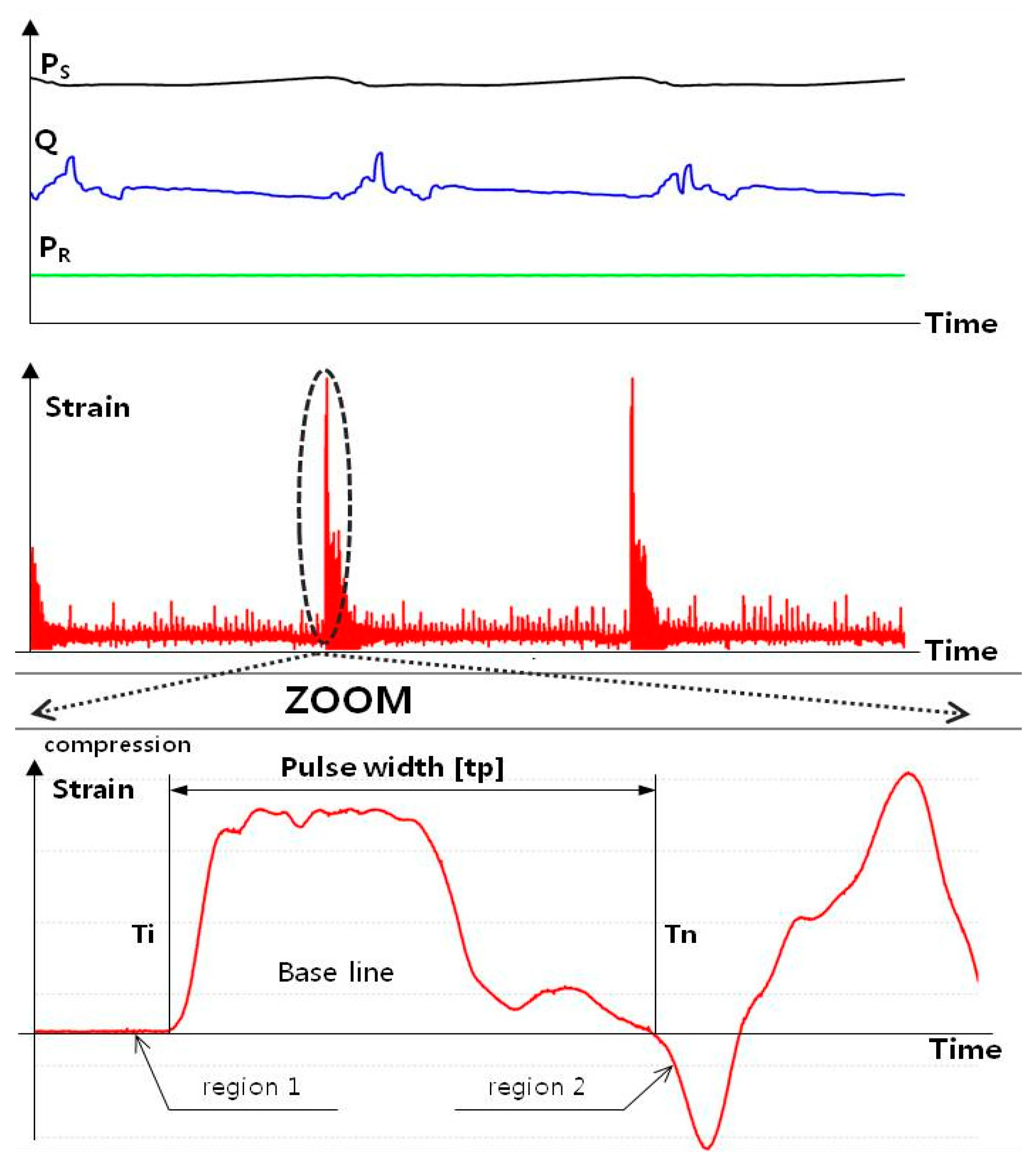
Figure 3.
A simple and generic neural network model.
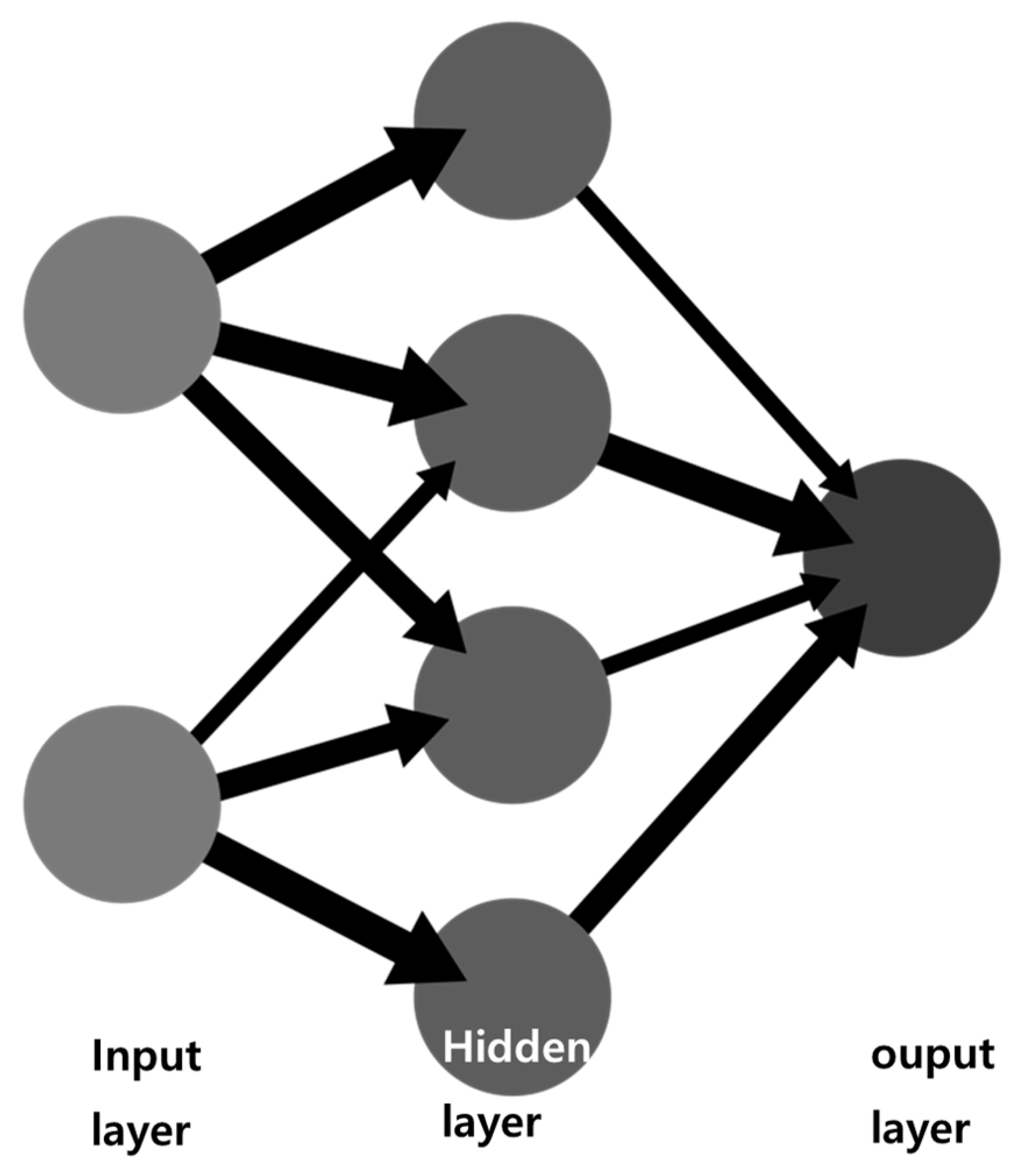
Figure 4.
Correlation analysis of hydraulic breaker parameters as: (a) a scatter plot of the correlation coefficient; (b) a value of the correlation coefficient.
Figure 4.
Correlation analysis of hydraulic breaker parameters as: (a) a scatter plot of the correlation coefficient; (b) a value of the correlation coefficient.
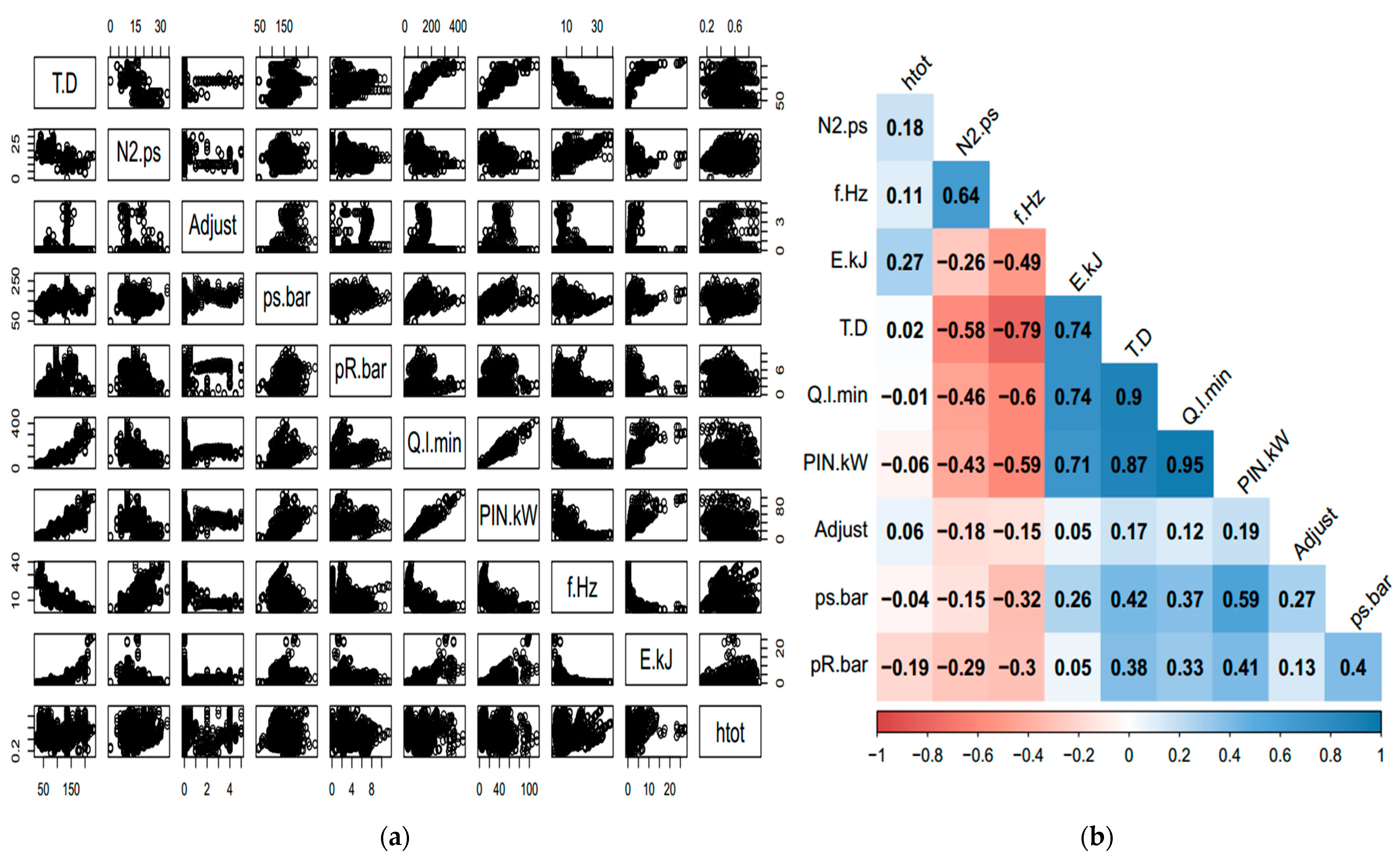
Figure 5.
Examples of applying sample hidden layers to a neural network model; (a) hidden layer 5; (b) hidden layer 1.
Figure 5.
Examples of applying sample hidden layers to a neural network model; (a) hidden layer 5; (b) hidden layer 1.

Figure 6.
Scatter plot of predicted versus measured impact energy of a hydraulic breaker as: (a) linear regression model (LR) of small-to-medium-class hydraulic breaker data set (MS–HB); (b) large-class hydraulic breaker data set (L–HB); (c) total size class data set (T–HB); (d) neural network min–max normalizer model (NN-MM) of small-to-medium-class hydraulic breaker (MS–HB) data set; (e) large-class hydraulic breaker data set; (f) total size class data set; (g) neural network Gaussian normalizer model (NN–GAU) of small-to-medium-class hydraulic breaker (MS–HB) data set; (h) large-class hydraulic breaker data set; (i) total size class data set.
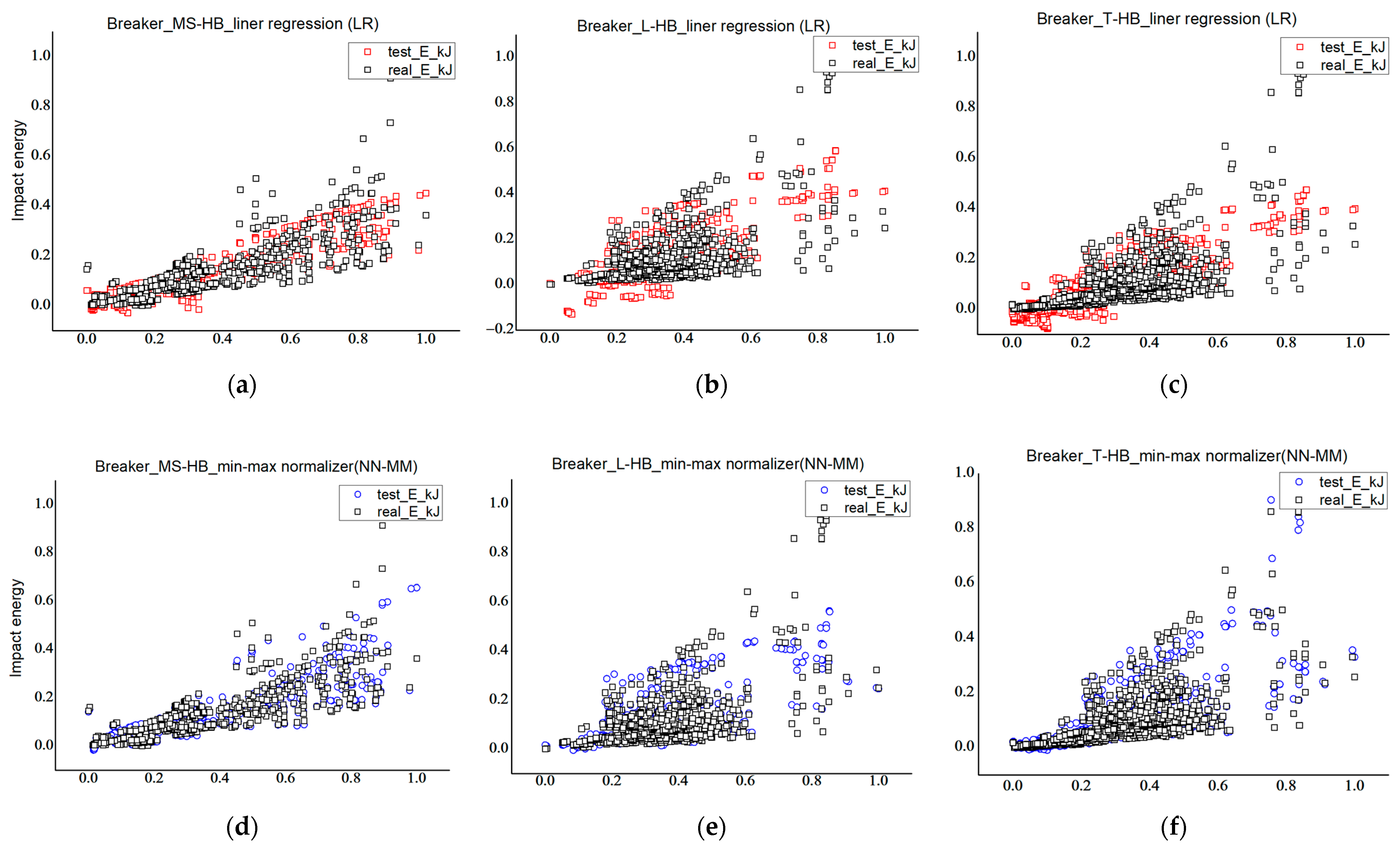
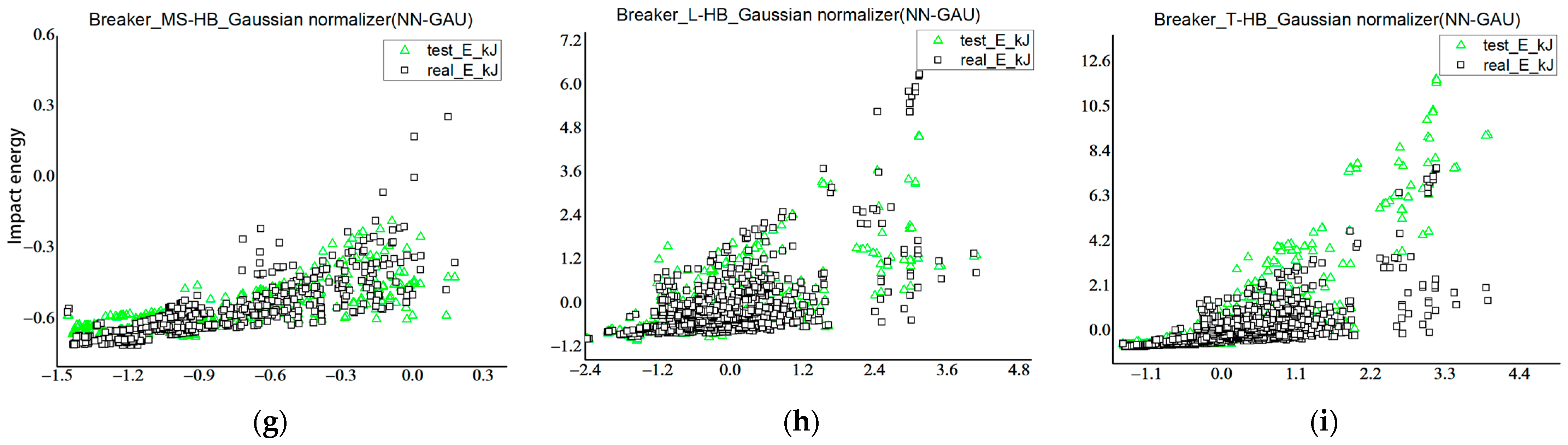
Figure 7.
The coefficient of determination and root mean square error (RMSE) of neural network Min–Max normalized versus neural network Gaussian normalized model for hidden layer number: (a) coefficient of determination of neural network Min–Max normalized (NN-MM) for hidden layer number; NN-MM total size class (T-HB), small-to-medium-class (MS-HB) and large-class hydraulic breakers (L-HB); (b) coefficient of determination of neural network with Gaussian normalized (NN-GAU) for hidden layer number; NN-GAU total size class (T-HB), small-to-medium-class (MS-HB) and large-class hydraulic breakers (L-HB); (c) root mean square error of NN mm for hidden layer number; NN mm total size class (T-HB), small-to-medium-class (MS-HB) and large-class hydraulic breakers (L-HB); (d) root mean square error of neural network with Gaussian normalized (NN-GAU) for hidden layer number; NN-GAU total size class (T-HB), small-to-medium-class (MS-HB) and large-class hydraulic breakers (L-HB).
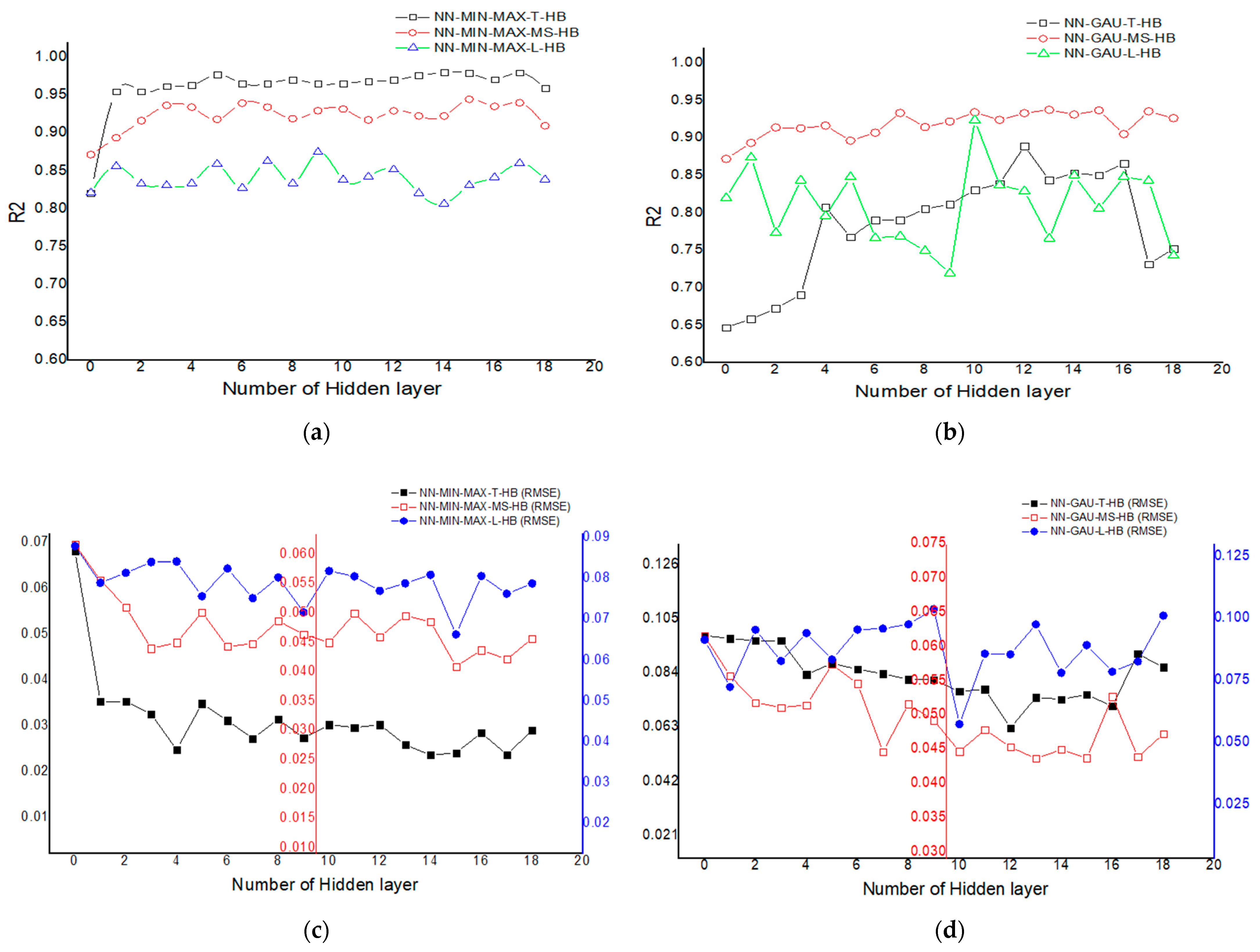
Figure 8.
A neural network regression test result diagram. Confidence interval calculation of best diagram and projected uncertainties (95 PPU) for NN–MM model: (a) Confidence interval calculation of best model; (b) 95% of projected uncertainties (95 PPU) for the NN–MM model.
Figure 8.
A neural network regression test result diagram. Confidence interval calculation of best diagram and projected uncertainties (95 PPU) for NN–MM model: (a) Confidence interval calculation of best model; (b) 95% of projected uncertainties (95 PPU) for the NN–MM model.
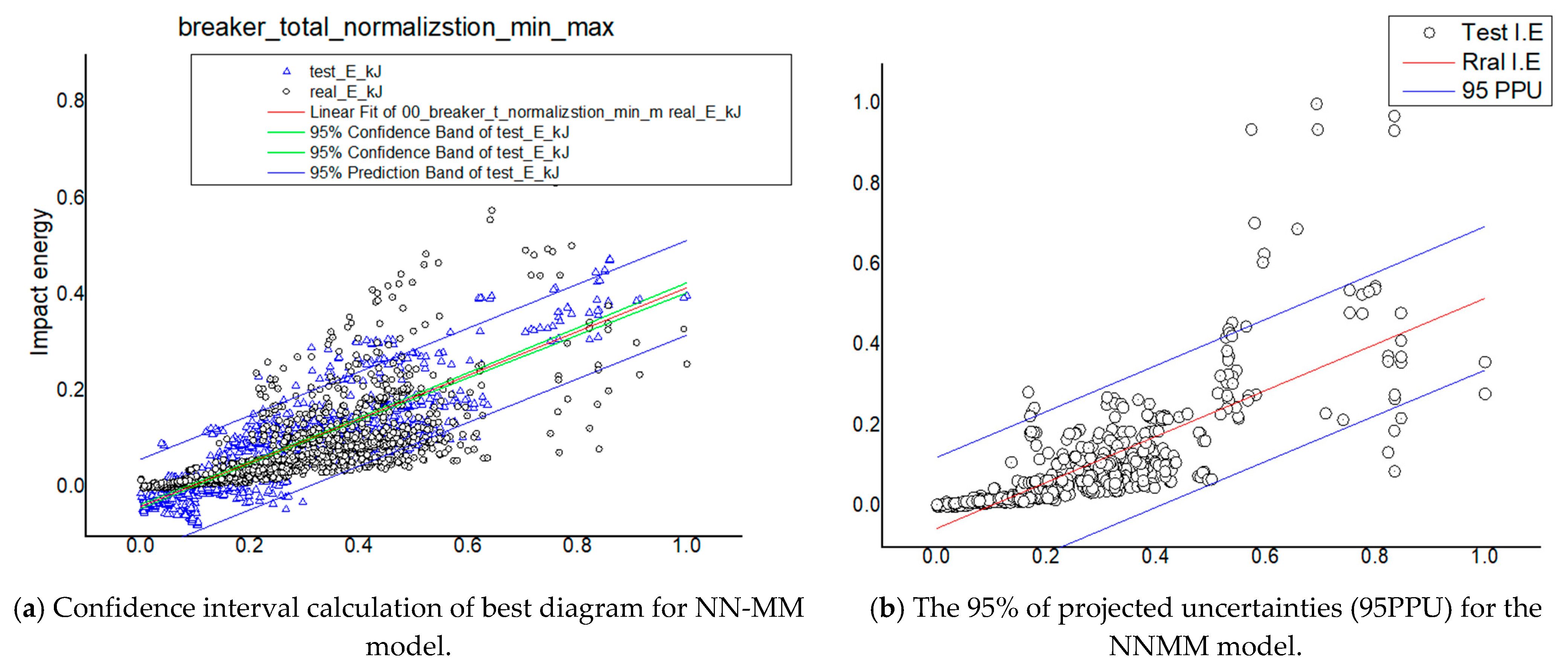
Figure 9.
An R2 comparison showing good NN–MM model performance and relative square error: (a) comparison of real data and predicted model R2 values, (b) relative square error (RSE) for NN–MM model.
Figure 9.
An R2 comparison showing good NN–MM model performance and relative square error: (a) comparison of real data and predicted model R2 values, (b) relative square error (RSE) for NN–MM model.


Table 1.
Performance test data of large-class hydraulic breaker.
| T-D [mm] | N2/ps [kg/cm2] | Adjust valve | ps/bar [bar] | pR/bar [bar] | Q/l/min [lpm] | PIN/kW [kw] | f/Hz [hz] | E/kJ 1 [k J] |
|---|---|---|---|---|---|---|---|---|
| … | … | … | … | … | … | … | … | … |
| 100 | 6.5 | 0 | 137.203 | 6.712 | 55.622 | 12.722 | 7.300 | 1.164 |
| 100 | 6.5 | 0 | 137.212 | 7.457 | 56.464 | 12.915 | 7.249 | 1.171 |
| 100 | 6.5 | 0 | 125.425 | 6.817 | 51.614 | 11.806 | 6.626 | 1.071 |
| 100 | 6.5 | 0 | 150.007 | 0.57 | 73.84 | 20.696 | 6.554 | 1.352 |
| 100 | 6.5 | 0 | 153.695 | 0.584 | 75.656 | 21.205 | 6.715 | 1.385 |
| … | … | … | … | … | … | … | … | … |
| 135 | 10 | 3.25 | 166.967 | 7.063 | 167.5 | 51.002 | 7.698 | 2.889 |
| 135 | 10 | 0 | 179.387 | 6.537 | 178.042 | 58.244 | 7.948 | 2.897 |
| 135 | 10 | 3.5 | 165.602 | 6.95 | 163.757 | 49.454 | 7.703 | 2.922 |
| 135 | 16 | 0 | 181.236 | 3.61 | 161.213 | 53.283 | 9.599 | 2.995 |
| 135 | 16 | 0 | 161.829 | 4.113 | 99.535 | 29.375 | 5.010 | 2.997 |
| … | … | … | … | … | … | … | … | … |
| 155 | 6 | 0 | 196.968 | 6.943 | 224.258 | 73.634 | 14.202 | 1.732 |
| 155 | 14 | 0.25 | 157.714 | 7.351 | 215.449 | 56.643 | 10.52 | 1.869 |
| 155 | 14 | 0.25 | 153.801 | 7.517 | 213.846 | 54.827 | 10.298 | 1.927 |
| 155 | 10 | 0 | 191.928 | 7.933 | 217.399 | 69.555 | 12.52 | 2.144 |
| 155 | 10 | 0 | 194.562 | 7.396 | 218.438 | 70.847 | 12.298 | 2.205 |
| … | … | … | … | … | … | … | … | … |
| 220 | 16 | 0 | 190.616 | 1.363 | 301.573 | 96.186 | 2.627 | 25.359 |
| 220 | 15.55 | 0 | 193.592 | 1.157 | 308.535 | 98.074 | 2.229 | 25.796 |
| 220 | 16 | 0 | 193.616 | 1.158 | 308.573 | 98.086 | 2.827 | 25.799 |
| 230 | 16 | 0 | 195.462 | 1.268 | 312.535 | 99.074 | 2.240 | 26.898 |
| 230 | 16.5 | 0 | 195.616 | 1.258 | 312.574 | 99.086 | 2.237 | 26.972 |
| … | … | … | … | … | … | … | … | … |
1 test data are the arithmetic average of five or more measurements.
Table 2.
Performance test data of small- and medium-class hydraulic breakers.
| T-D [mm] | N2/ps [kg/cm2] | Adjust valve | ps/bar [bar] | pR/bar [bar] | Q/l/min [lpm] | PIN/kW [kw] | f/Hz [hz] | E/kJ 1 [k J] |
|---|---|---|---|---|---|---|---|---|
| … | … | … | … | … | … | … | … | … |
| 25 | 16 | 0 | 105.641 | 0.052 | 21.956 | 6.250 | 21.791 | 0.416 |
| 25 | 16 | 0 | 117.379 | 0.058 | 24.395 | 6.945 | 24.212 | 0.371 |
| 30 | 17 | 0 | 111.995 | 0.089 | 29.085 | 7.231 | 24.593 | 0.817 |
| 30 | 18 | 0 | 122.788 | 0.097 | 31.887 | 7.928 | 26.964 | 0.896 |
| 30 | 17 | 0 | 121.580 | 0.125 | 29.221 | 7.126 | 28.931 | 0.970 |
| … | … | … | … | … | … | … | … | … |
| 50 | 14 | 0 | 134.162 | 0.095 | 18.827 | 4.241 | 11.631 | 3.350 |
| 50 | 16 | 0.25 | 134.163 | 0.085 | 18.838 | 4.250 | 11.922 | 3.366 |
| 50 | 15 | 0 | 134.743 | 0.087 | 18.920 | 4.269 | 11.974 | 3.376 |
| 50 | 14 | 0 | 135.344 | 0.085 | 19.004 | 4.288 | 12.027 | 3.391 |
| 50 | 15 | 0 | 135.929 | 0.086 | 19.086 | 4.306 | 12.079 | 3.405 |
| … | … | … | … | … | … | … | … | … |
| 80 | 14 | 0 | 156.378 | 2.787 | 66.335 | 17.292 | 12.639 | 4.998 |
| 80 | 13 | 0.5 | 138.297 | 0.116 | 101.453 | 23.389 | 19.432 | 5.002 |
| 80 | 16 | 0 | 167.263 | 2.858 | 59.226 | 16.514 | 12.590 | 5.476 |
| 80 | 17 | 0 | 136.350 | 0.104 | 95.959 | 21.811 | 20.341 | 5.723 |
| 80 | 16 | 0 | 164.464 | 2.361 | 60.966 | 16.714 | 12.488 | 5.724 |
| … | … | … | … | … | … | … | … | … |
| 95 | 14 | 0.5 | 146.140 | 8.652 | 89.426 | 23.833 | 18.079 | 6.169 |
| 95 | 16 | 0.5 | 143.905 | 8.736 | 91.242 | 23.945 | 18.218 | 6.481 |
| 95 | 14 | 0.5 | 155.947 | 10.506 | 101.611 | 28.897 | 19.349 | 6.547 |
| 95 | 16 | 0.5 | 168.624 | 10.138 | 104.425 | 32.112 | 19.714 | 7.271 |
| 95 | 14 | 0 | 156.045 | 7.452 | 98.351 | 27.988 | 12.722 | 8.234 |
| … | … | … | … | … | … | … | … | … |
1 test data are the arithmetic average of five or more measurements.
Table 3.
Hydraulic breaker data summary.
| T-D | N2/ps | Adjust | ps/bar | pR/bar | Q/l/min | PIN/kW | f/Hz | E/kJ | ||
|---|---|---|---|---|---|---|---|---|---|---|
| Small and medium-class of hydraulic breaker (MS-HB) | MEAN 1 | 65.163 | 18.587 | 0.096 | 138.424 | 2.049 | 53.578 | 13.802 | 16.705 | 4.360 |
| STDEV 2 | 19.093 | 4.627 | 0.282 | 27.334 | 1.776 | 28.502 | 8.355 | 7.085 | 3.300 | |
| MIN | 56.799 | 13.000 | 0.000 | 56.799 | 0.052 | 10.683 | 1.306 | 5.687 | 0.371 | |
| MAX | 212.468 | 34.000 | 2.000 | 212.468 | 11.494 | 131.001 | 35.882 | 38.820 | 17.400 | |
| MEDN 3 | 70.000 | 16.000 | 0.000 | 139.040 | 2.029 | 47.006 | 11.916 | 14.953 | 3.438 | |
| Large-class of hydraulic breaker (L-HB) | MEAN | 142.878 | 12.420 | 0.658 | 167.581 | 4.362 | 159.272 | 45.898 | 6.927 | 3.735 |
| STDEV | 25.011 | 3.854 | 1.370 | 28.322 | 2.500 | 61.848 | 16.968 | 2.360 | 3.679 | |
| MIN | 100.000 | 0.000 | 0.000 | 42.969 | 0.074 | 49.624 | 5.642 | 1.938 | 0.334 | |
| MAX | 230.000 | 23.000 | 5.000 | 278.434 | 10.582 | 435.952 | 115.255 | 16.631 | 27.102 | |
| MEDN | 135.000 | 12.000 | 0.000 | 170.575 | 4.851 | 149.590 | 44.390 | 7.042 | 2.685 |
1 MEAN; Average value of each item data, 2 STDEV; Standard deviation of each item data, 3 MEAN: Median value of each item’s data.
Table 4.
Performance values of predicted test data.
| Testing Algorithm | T-HB | MS-HB | L-HB | |||
|---|---|---|---|---|---|---|
| R2 | RMSE | R2 | RMSE | R2 | RMSE | |
| Linear regression (LR) | 0.82067 | 0.06812 | 0.88079 | 0.05861 | 0.84111 | 0.07434 |
| Neural network: min–max normalize (NN-MM) | 0.98023 | 0.02359 | 0.94510 | 0.04093 | 0.89130 | 0.06633 |
| Neural network: Gaussian normalize (NN-GAU) | 0.88959 | 0.06272 | 0.93796 | 0.04366 | 0.92404 | 0.40246 |
Disclaimer/Publisher’s Note: The statements, opinions and data contained in all publications are solely those of the individual author(s) and contributor(s) and not of MDPI and/or the editor(s). MDPI and/or the editor(s) disclaim responsibility for any injury to people or property resulting from any ideas, methods, instructions or products referred to in the content. |
© 2023 by the authors. Licensee MDPI, Basel, Switzerland. This article is an open access article distributed under the terms and conditions of the Creative Commons Attribution (CC BY) license (https://creativecommons.org/licenses/by/4.0/).
Share and Cite
MDPI and ACS Style
Kim, S.-H.; Park, J.-W.; Kim, J.-H. Comparative Analysis of Machine Learning Approaches to Predict Impact Energy of Hydraulic Breakers. Processes 2023, 11, 772. https://doi.org/10.3390/pr11030772
AMA Style
Kim S-H, Park J-W, Kim J-H. Comparative Analysis of Machine Learning Approaches to Predict Impact Energy of Hydraulic Breakers. Processes. 2023; 11(3):772. https://doi.org/10.3390/pr11030772
Chicago/Turabian StyleKim, Sung-Hyun, Jong-Won Park, and Jae-Hoon Kim. 2023. "Comparative Analysis of Machine Learning Approaches to Predict Impact Energy of Hydraulic Breakers" Processes 11, no. 3: 772. https://doi.org/10.3390/pr11030772
Note that from the first issue of 2016, this journal uses article numbers instead of page numbers. See further details here.