CFD Modeling of an H-Type Darrieus VAWT under High Winds: The Vorticity Index and the Imminent Vortex Separation Condition

Abstract

This study introduces a Vorticity Index (VI) and an Imminent Vortex Separation Condition (IVSC), which are considered valuable indicators to quantify the vorticity impact on vertical axis wind turbines (VAWTs) operation. The VI and IVSC are specifically applied to a H-Darrieus vertical axis wind turbine (VAWT). Findings show that these two parameters display a direct relationship with the aerodynamic forces that govern the performance of this type of VAWT. This analysis is accomplished via 2D-CFD simulations of a H-Darrieus with a symmetrical NACA 0018, powered by high winds (8 and 20 m/s), by using a Shear Stress Transport SST k-ω model. The 2D model used is validated for Class II winds (8 m/s), for tip speed ratios (λ) ranging from 0.4 to 0.9. Power coefficients (C_p) predictions are close to those obtained with both 3D simulations and with experimental data, reported in the technical literature. It is found with the numerical simulations developed, that despite the significant increase of the average rotor overall torque values, when the wind speed is augmented from 8 m/s to 20 m/s, the energy extracted by the rotor seems to be moderately lessened by the amplified turbulence and vorticity.

1. Introduction

The continuous decrease of natural resources available for energy production and the unwanted CO₂ emissions produced from fossil fuels combustion, have generated great interest in the development of alternative and renewable energies [1]. According to the latest report from the global company BP, considering an accelerated scenario, by the year 2050 alternative and renewable energies might even become the largest source of energy in the world, comprising approximately 60% of the global market [2]. These types of energies consist of solar, biomass, geothermal, hydroelectric and wind [3]. Being wind energy a favored option for planners and national governments [3,4,5]. Compared to conventional energy sources, wind power is positioned as one of the most important sources of renewable energy and the high potential of its use in electric power generation [5,6,7].

Furthermore, wind energy is considered to provide unique opportunities for the implementation of small scale and decentralized hydrogen production technologies [8,9]. Wind energy contributes to the first step in an integrated process, where it can be converted into electrical power. Electrical energy can be used later for the production of hydrogen via photocatalysis or electrolysis [10].

Given these incentives, in the last decades, the extraction of energy from the wind through wind turbines has seen an accelerated development. The growing investment in researching these technologies has resulted in the development of increasingly powerful turbines designs at more affordable prices. These designs include both horizontal axis wind turbines (HAWTs) as well as vertical axis wind turbines (VAWTs) [11].

In spite of most implemented wind turbines have been the HAWT designs, given their greater efficiency while compared to VAWTs [12,13], the HAWTs still show certain disadvantages such as (a) high maintenance costs, (b) location requirements [4,14] and (c) wind direction dependence [15]. In this respect, VAWTs can be considered a better option than HAWTs under certain operating conditions because of their: (i) variable wind direction potential, (ii) adaptability for domestic installations, (iii) compactness, and (iv) capability to operate under severe turbulent flow conditions [14,16], normally present under high winds. The main differences between VAWT and HAWT configurations are summarized in

Table 1. Comparison of Parameters between VAWT and HAWT.

	Vertical Axis Wind Turbine (VAWT)	Horizontal Axis Wind Turbine (HAWT)
Efficiency	Lower	Higher
Space Efficiency a,b	Higher	Lower
Wind Direction a,b	Independent	Dependent
Yaw mechanism b	No	Yes
Self-Starting b	No	Yes
Height from ground b	Small	Large
Tower Sway b	Small	Large
Generator location b	Ground Level	Not Ground Level Required
Installation Cost a,b	Lower	Higher
Maintenance Cost a,b	Lower	Higher
Shadow Flickering b	Less	More
Noise a,b	Low	High
Bird/bat safety a,b	High	Low

^a [17], ^b [18].

.

Given their reported advantages, VAWTs have become increasingly relevant in the field of wind energy research, as can be seen in the increasing number of bibliographic publications available for each of these configurations (Figure 1). In general, the research areas of primary interest regarding VAWTs are concerned with improving turbine rotor efficiency, through aerodynamic analysis and wind tunnel experimentation [17]. In this regard, different designs have been evaluated to reduce the problems that affect their performance. However, aerodynamics analysis and experiments in wind tunnels can be costly and require significant research time [19].

Thus, computational models that allow establishing the behavior of VAWTs, have become one of the preferred tools of both industry and researchers in this field [20,21]. These computational methods can be used to establish vorticity parameters, which can significantly help to quantify the influence of vorticity on VAWT performance. To accomplish this the main objectives of this work are the following:

• To implement a Vorticity Index (VI), defined as the ratio between the leading-edge vorticity (LEV) and the trailing-edge vorticity (TEV), to quantify vorticity in the VAWTs.
• To develop this study using a 2D model validated with experimental data reported in the literature [22].
• To establish a relationship between the Vorticity Index (VI) and the Imminent Vortex Separation Condition (IVSC) with the VAWT extracted energy, for a VAWT functioning at 8 m/s and 20 m/s.

2. Numerical Simulation

2.1. Physical Model

One of the most studied VAWT designs is the Darrieus type H (H-Darrieus) wind turbine. This design mainly consists of 3 aerodynamic profile blades attached to a vertical rotating shaft, which are driven by the force of the wind that hits them [23]. In recent years, different CFD simulations of H-Darrieus wind turbines have been carried out implementing 2D models [24,25,26,27] and 3D models [6,28,29]. In the case of most of these simulations, the shaft is usually not included in the geometric model, as shown in Figure 2.

As reported in

Table 2. Design Parameters of the H-Darrieus Wind Turbine [22].

Parameter	Symbol	Value
Rotor Diameter [m]	$D$	0.8
Blade Airfoil	-	NACA 0018
Blade Shape	-	Straight
Chord Length [m]	$c$	0.2
Rotor Height [m]	$H$	0.8 m (1 m adopted for 2D simulation)
Blades Number	$N$	3
Solidity	$\sigma$	0.75

Note: Solidity, $\sigma$ = $\frac{N c}{D}$.

, the design parameters and dimensions of the geometric model implemented in this work corresponded to the dimensions of a H-Darrieus wind turbine that was experimentally tested by Elkhoury et al. [22] using a NACA 0018 blade. This specific blade configuration was selected given the abundant experimental and simulation data for VAWTs with NACA 0018.

2.2. Computational Domain

For H-Darrieus wind turbine CFD simulations, two domains of interest can normally be considered: (i) a fixed domain which represents the control volume and (ii) a rotating domain inside of which, the rotor is accounted for. In this work, the fixed domain corresponds to a rectangle of 20 m × 8 m, and the rotating domain involves a 1.6 m or a $2D$ diameter circle (Figure 3). It can be noticed that the center of the rotor was located at $10D$ from the inlet boundary and at $15D$ from the outlet boundary. This was determined in order to ensure the correct development of the wake effect [6], which may lead to an underestimation of the fluid velocity and an overestimation of the turbulence [30].

The boundary conditions: inlet, outlet, lateral sides, blades, and contact region, for rotating and fixed domains were set by using the velocity inlet, the pressure outlet, the symmetry plane, non-slip walls, and sliding interface, respectively.

2.3. Setting Up

In this work, the commercial software ANSYS 19.1 Fluent was selected as the CFD simulation package, to solve the flow equations. The continuity Equation (1) and the momentum Equation (2) used to solve URANS simulations in the ANSYS Fluent software are shown below [31,32]:

$$\frac{\partial {\overline{u}}_i}{\partial x_i}=0$$

(1)

$$\frac{\partial {\overline{u}}_i}{\partial t}+\frac{\partial }{\partial x_j}\left( {\overline{u}}_i{\overline{u}}_j\right)=-\frac{1}{\rho }\frac{\partial \overline{p} }{\partial x_i}+\frac{\partial }{\partial x_j}\left(v \frac{\partial {\overline{u}}_i}{\partial x_j}-{\overline{u}}^{\prime }{}_i{\overline{u}}^{\prime }{}_j\right)$$

(2)

where, ${\overline{u}}_i$ and ${\overline{u}}_j$ are the mean values of velocity in the axial system of coordinates, $u_{ i}^{\prime }$ and $u_{ j}^{\prime }$ its fluctuating components,$\overline{p}$ is the mean pressure, $v$ is the kinematic viscosity, $\rho$ is the density of the fluid and $t$ is the time. It is important to point out that the term ${\overline{u}}^{\prime }{}_i{\overline{u}}^{\prime }{}_j$, commonly represents the Reynolds stress tensor, which depends on the turbulence model selected [32].

For URANS calculations, the pressure-based solver was utilized while the pressure-velocity coupling was handled using coupled algorithm. The second-order upwind scheme was used for the spatial discretization of the pressure, the turbulence model, and the momentum equations. The main settings implemented for all the simulations are listed in

Table 3. Details of Numerical Set-Up.

Parameter	Symbol	Value
Viscous Model	SST k-$\mathsf{\omega }$	k-$\mathsf{\omega }$ Shear Stress Transport
Air Density	$\rho$	1.225 kg/m3
Air Viscosity	$\mu$	1.79 × 10−5 Pa s
Air Velocity	$U_{\infty }$	8 m/s, 20 m/s
Turbulent Intensity		1%
Tip Speed Ratio	λ	0.5–1.5
Solver Type		Pressure-Based
Calculation algorithm		Coupled
Spatial Discretization		2nd
Time discretization		According to λ, calculated to achieve 2° of rotation per time step
Residuals		1 × 10−4

Note: Tip Speed Ratio, $\lambda =\frac{R \omega }{U_{\infty }}$.

.

Turbulence Model

During RANS and URANS simulations, different numerical models can be employed to determine the eddy viscosity turbulence [21,33]. These turbulence models used for CFD simulation include: (a) a one-equation Spalart-Allmaras model, (b) two-equation models such as k-ε (RNG), Realizable k-ε (RKE) and SST k-$\mathsf{\omega }$ models, (c) three equations model such SST k-$\mathsf{\omega }$ with intermittency (SSTI). Comparisons of their results with experimental data have been reported by [17,34,35]. In agreement with the previous research [31,36], the Shear Stress Transport (SST) based models have been demonstrated as being the most accurate. Among them, the SST k-$\mathsf{\omega }$ model was shown to be effective for VAWT CFD simulations. This is mainly because the SST k-$\mathsf{\omega }$ model performs well in the treatment of the boundary layer over the blades and works well in the air free-flowing areas [16,37,38]. Therefore, the SST k-$\mathsf{\omega }$ model was chosen for this study.

2.4. Meshing

The computational mesh used in the present study was developed using the ANSYS 19.1 meshing tool. To determine the best mesh size in terms of computational cost and accuracy, the influence of the computational grid on the main calculations was evaluated. In this study, three different unstructured computational meshes were tested for a set wind speed ($U_{\infty }$) of 8 m/s at a tip speed ratio ($\lambda$) of 1. Following this analysis, the medium mesh was selected as the optimal one. This was determined after obtaining an average power coefficient ($C_p)$ value difference lower than 1.25% when testing the finest mesh. The number of elements within the computational domains, for each mesh, and their respective average $C_p$ values, are reported in

Table 4. Mesh Independence Test for λ = 1.

		Mesh Set
		Coarse	Medium	Fine
Face Sizing	Fixed Domain Element Size [m]	0.120	0.080	0.060
	Rotor Domain Element Size [m]	0.012	0.0073	0.0053
Edge Sizing	Interface Element Size [m]	0.011	0.0069	0.0049
	Number of Divisions around Blades Surface	480	600	600
Elements Number	Fixed Domain	29,008	75,226	143,289
	Rotor Domain	62,416	125,564	216,843
	Total	91,424	200,790	360,132
Power Coefficient	$C_p$	0.196	0.200	0.202
	%Difference of $C_p$ with respect to the Fine Mesh	−3.06%	−1.23%	/

.

Similar approaches for grid dimensioning were used for the three meshes considered in the present study, as follows: (a) First, the triangle method was applied for both domains, (b) Then, the rotating domain was refined by using a face sizing, (c) Following this step, the interface between the fixed domain and the rotating domain was refined by using an edge sizing, (d) Finally, the blades’ surfaces were grid sized by increasing the number of elements around them and by creating an adequate inflation number for each of them. This was done to guarantee a $y$+ value < 1. This approach was considered to capture the viscous sublayer, as suggested by [20,30]. It is important to mention that the selected medium mesh size (Figure 4), complies with two conditions: (a) the 0.36 lowest orthogonal quality for the whole mesh is larger than 0.1 and (b) the 0.79 maximum skewness for the whole mesh is smaller than the 0.95 maximum advised [38].

2.5. Angular Marching Step

The timestep size is an important parameter when developing unsteady simulations, since it has a great influence on the final values obtained [37]. In this regard, the simulation for $U_{\infty }$ = 8 m/s at $\lambda$ = 1 was considered as the base case, with three different time steps being evaluated during ten consecutive H-Darrieus wind turbine rotor rotations. This approach was judged to be reliable in order determine the adequate time step to generate the most consistent $C_p$ results, at the lowest computational cost. As a result, the three timesteps evaluated for the base case were 0.003491 s, 0.001745 s and 0.000873 s, which corresponded to angular marching steps (${\Delta }\alpha$) of 4°, 2° and 1°, respectively.

As shown in Figure 5, for each ${\Delta }\alpha$, the $C_p$ value stabilization required a different number of simulated rotations, being the case when ${\Delta }\alpha$ = 4 the one that required the smallest number of simulated rotations. On the other hand, although when ∆α = 2°, a higher number of simulated rotations was required to provide stabilized $C_p$ values than when using ∆α = 4°, its final $C_p$ value showed a 3% difference only versus the $C_p$ value calculated when ∆α = 1°, as reported in

Table 5. Timestep Independence Test for λ = 1.

Time Step	$\mathbf{Angular} \mathbf{Marching} \mathbf{Step} \left(\mathsf{\Delta }\mathit{\alpha }\right)$	${\mathit{C}}_{\mathit{m}}$	${\mathit{C}}_{\mathit{p}}$	$\%\mathbf{Difference} \mathbf{of} {\mathit{C}}_{\mathit{p}}$ with Respect to Smallest Time Step
0.003491 s	4°	0.200	0.200	−12%
0.001745 s	2°	0.220	0.220	−3%
0.000873 s	1°	0.227	0.227	<0.1%

. Thus, ∆α = 2° was considered a good compromise as an angular marching step, reducing computational cost without considerably compromising the accuracy of the results.

3. Results and Discussion

In this work, all calculations were performed using the MATLAB R2021a Software, based on the values generated with the ANSYS 19.1 Fluent solver. The power coefficient (3) was calculated using the torque results obtained via CFD simulations. A minimum of eight rotor rotations were considered for all the simulations. This to guarantee the consistency of numerical calculations between rotations, as recommended in the technical literature [20]. The average $C_p$ values were then estimated and presented in this section, for $U_{\infty }$ = 8 m/s and $U_{\infty }$ = 20 m/s, at various tip speed ratios ($\lambda$) of interest.

$$C_p=\frac{P_{turbine}}{P_{wind}}=\frac{T \omega }{\frac{1}{2}\rho U_{\infty }^3\left(2R H\right)}$$

(3)

where T represents the mechanical torque, ${\omega }$ denotes the rotational speed of the rotor, $U_{\infty }$ stands for the free wind speed, $\rho$ is the air density and, $R$ and $H$ are radius and height of the rotor, respectively.

Considering the convergence of the results between rotations, the behavior of the torque, the power coefficient, and the drag and lift forces were reported for the last simulated H-Darrieus wind turbine rotation for both wind speeds, and this for two different $\lambda$ values of 0.5 and 0.9. This was done in order to analyze the influence of the wind speed on the general aerodynamics of the proposed H-Darrieus wind turbine. Finally, graphical contours were produced at various stages of the H-Darrieus wind turbine operation, to illustrate the effects of vortex shedding on the performance of the wind turbine and to relate them to the vorticity index proposed in this study.

3.1. Model Validation

To validate the 2D CFD simulations of the H-Darrieus wind turbine carried out in this study, the first section of this article compares the calculated average $C_p$ values with the values reported by Ma et al. [37], at various tip speed ratios ($\lambda$). In their work, the authors evaluated the same rotor configuration for a wind speed ($U_{\infty }$) of 8 m/s with runs developed in a wind tunnel and by using 3D CFD simulations. Although 2D simulations can generate certain discrepancies with respect to the experimental results, such simulations can provide a reliable representation of the flow in the mid-plane of the turbine, at a considerably lower computational cost than 3D simulations and even 2.5D simulations [17,27]. The differences obtained in each type of CFD simulation with respect to the data obtained experimentally, are reported in

Table 6. Power Coefficient Comparison of 2D SST k-$\mathsf{\omega }$ Simulation with Experimental Data and 3D SST k-$\mathsf{\omega }$ Simulation Results.

	$\mathbf{Power} \mathbf{Coefficient} \left({\mathit{C}}_{\mathit{p}}\right)$
$\mathit{\lambda }$	Experimental Results [37]	2D SST k-$\mathsf{\omega }$ (This Work)	Relative Error 2D vs. Exp	3D SST k-$\mathsf{\omega }$ [37]	Relative Error 3D vs. Exp
0.4	0.028	0.030	5.9%	0.030	5.5%
0.5	0.040	0.036	−10.6%	0.048	19.6%
0.7	0.073	0.053	−27.5%	0.079	8.6%
0.8	0.101	0.108	7.2%	0.105	4.7%
0.9	0.128	0.157	22.9%	0.132	3.1%
1.0	0.167	0.220	31.5%	0.159	−4.7%
1.2	0.190	0.326	71.4%	0.184	−3.3%
1.3	0.195	0.355	81.9%	0.191	−2.0%
1.4	0.186	0.375	101.5%	0.191	2.5%
1.5	0.169	0.385	128.0%	0.180	6.0%

.

As shown in Figure 6, simulations predictions of average $C_p$ values for a 2D model were greater than those obtained in 3D simulation. While 2D simulations may provide a somewhat limited description of the complex dynamics of the flow, around the wind turbine [19,29,39], for tip speed ratios ranging from 0.4 to 0.9, the average relative error is about +/−9.27%, with a maximum relative error value of 27.5%. Therefore, this approach is acceptable for the validation of the vorticity index (VI) within the expected level of confidence of the experimental data, when tip speed ratios are below 0.9 values. For λ values larger than 0.9, observed 2D simulations results could not adequately represent the experimental data, and therefore were not considered in the present analysis.

3.2. Influence of High Winds

3.2.1. Wind Speed Effect on Overall Torque—Convergence Criteria

The stability criteria for the average rotor overall torque values, following two consecutive revolutions, was achieved for both low (8 m/s) and high (20 m/s) wind speeds. As shown in Figure 7, a difference smaller than 1% in the average toque value between two subsequent rotations was achieved for all the tip speed ratios evaluated, as suggested by [40]. In this respect, a significant increase of about seven to eight times, in the average rotor overall torque values was noticed when the wind speed increased from 8 m/s to 20 m/s. In the case of $U_{\infty }$ = 8 m/s simulations (Figure 7a), this value varied between 0.93 N m (for $\lambda$ = 0.4) and 2.2 N m (for $\lambda$ = 0.9), while in the case of the $U_{\infty }$ = 20 m/s simulations (Figure 7b), the average rotor overall torque varied between 7.2 N m (for $\lambda$ = 0.4) and 16.7 N m (for $\lambda$ = 0.9).

Regarding VAWTs, the upcoming sections of the present article, reports the influences of drag and lift forces on the performance of the H-Darrieus wind turbine’s rotor. This is accomplished by considering that the overall torque of the turbine largely depends on the positions of the blades and the dominant forces on the rotor during its rotations, with this either being the lift force or the drag force [32,39].

3.2.2. Wind Speed Effect on Drag and Lift Forces

One of the main advantages of VAWTs is that they do not require a specific wind orientation mechanism to operate (Table 1), which is of great importance in regions of high rotating winds. It is, however, also well known that the aerodynamic forces during VAWTs operation are cyclic and contribute to fatigue and low power coefficients ($C_p$) while compared to the ones obtained in HAWTs.

In the case of an H-Darrieus wind turbine, the aerodynamic forces generated on the sectional profile of the blades as consequence of airflow through the turbine rotor, are significantly influenced by the azimuthal angle (θ) [27] and the angle of attack α of the wind. These forces, generally referred to as the lift forces (FL) and drag forces (FD) correspond to the force perpendicular to the flow and the force in the direction of the wind relative flow velocity (W), respectively [41]. Thus, based on FL and FD, the accountable forces of the torque such as normal forces and the tangential forces, can be established as described in Figure 8.

Figure 9 and Figure 10 report the drag and the lift forces on the 3 blades of the H-Darrieus wind turbine for the same wind speed ($U_{\infty }$ = 8 m/s) at two different tip speed ratios: $\lambda$ = 0.5 and $\lambda$ = 0.9. Furthermore, these figures show not only the displacements of the maximum and minimum values of these aerodynamic forces but also the variations in their cyclical behavior, both in terms of magnitude, and in terms of distribution over a rotational period. Then, one can notice that in the case for the drag forces, the maximum and minimum values on the main blade at $\lambda$ = 0.5 (Figure 9a) are reached at θ = 60° and θ = 176°, respectively. At $\lambda$ = 0.9 (Figure 9b), there is a peak displacement, and these values are reached at θ = 84° and θ = 162°, respectively. On the other hand, in the case for lift forces, the displacement effect is small, and the maximum and minimum values on the main blade are reached at θ = 118° and θ = 50°, respectively when $\lambda$ = 0.5 (Figure 10a), and at θ = 114° and θ = 54°, respectively when $\lambda$ = 0.9 (Figure 10b). Thus, it can be observed that at higher $\lambda$, the drag forces on the blades increase significantly (Figure 9). Furthermore, in the case of the lift forces (Figure 10), an effect of λ on the second negative peak of the distribution in the θ = 60°–180° azimuthal range is evidenced. One can see that this second minimum (−20 N) is attained at an earlier azimuthal angle, as compared to the angle reached when λ = 0.5 (−10 N).

On the other hand, when the behavior of the drag force (Figure 11) and the lift force (Figure 12) on the main blade for both wind speeds are compared, they show practically identical distributions, with the maximum and the minimum values of these two forces on the main blade being reached approximately at the same azimuthal angles (θ).

In the case of a fixed pitch blade, as the angle of attack increases, “static stall” conditions are reached, with flow separation and draft forces being greater than lift forces. However, due to the rotation of a VAWT, there is a pitching oscillation of the blades that results in a “dynamic stall” condition. This condition is characterized by a vortex generation that starts at the leading edge of the blade and is shed later, with lift and drag forces fluctuating [25] as the angle of attack rapidly changes. Thus, as the wind turbine rotate, different azimuthal angles are reached and the angle of attack (α) on each blade influences drag and lift forces. The influence of $\lambda$ and the azimuthal position (θ) on the angle of attack (α) can be described as proposed by Laneville & Vittecoq [42]:

$$tan \left(\alpha \right)=\frac{Sin \left(\theta \right)}{\left(Cos \left(\theta \right)+\lambda \right)}$$

(4)

Then, when the main blade (Blade 1) starts to turn counterclockwise from the θ = 0° angular position (Figure 8), a “dynamic stalling” effect seems to start to develop with lift forces decreasing and drag forces increasing progressively. One can observe that for Blade 1, lift and drag force minimum and maximum values take place between θ = 50° and θ = 64° with a lift force magnitude change from −30 N for $U_{\infty }$ = 8 m/s to −190 N for $U_{\infty }$ = 20 m/s (Figure 12a). There are no significant changes in this azimuthal angle, when $\lambda$ increases from 0.5 to 0.9 (Figure 12b). In addition, and at the same conditions, drag forces on Blade 1 show a peak increase from 38 N for $U_{\infty }$ = 8 m/s to 250 N for $U_{\infty }$ = 20 m/s (Figure 11a) 280 N for $U_{\infty }$ = 20 m/s is even reached when $\lambda$ increases from 0.5 to 0.9 (Figure 11b).

A summary of both the maximum and the minimum drag and lift forces for Blade 1 and their corresponding angles of attack, for both $U_{\infty }$ = 8 m/s and $U_{\infty }$ = 20 m/s at the two $\lambda$ of interest, is reported in

Table 7. Summary of Maximum and Minimum Drag and Lift Forces on the Blade 1 for $U_{\infty }$ = 8 m/s and $U_{\infty }$ = 20 m/s at both $\lambda$ = 0.5 and $\lambda$ = 0.9.

	λ	θ [Degrees]	α [Degrees]
Figure 9 Drag Forces $U_{\infty }$ = 8 m/s	0.5	60	40.9	Max. Drag
		176	−8.0	Min. Drag
	0.9	84	44.7	Max. Drag
		162	−80.6	Min. Drag
Figure 10 Lift Forces $U_{\infty }$ = 8 m/s	0.5	50	33.8	Min. Lift
		118	88.0	Max. Lift
	0.9	54	28.5	Min. Lift
		114	61.6	Max. Lift
Figure 11 Drag Forces $U_{\infty }$ = 20 m/s	0.5	64	43.8	Max. Drag
		180	0.0	Min. Drag
	0.9	90	48	Max. Drag
		164	−77.5	Min. Drag
Figure 12 Lift Forces $U_{\infty }$ = 20 m/s	0.5	50	33.8	Min. Lift
		120	90	Max. Lift
	0.9	54	28.5	Min. Lift
		116	62.8	Max. Lift

. One can observe, on this basis, that the maximum position of the drag forces for $U_{\infty }$ = 8 m/s shifts from θ = 60° to θ = 84° as the tip speed ratio increases from 0.5 to 0.9. This change can also be seen when $U_{\infty }$ = 20 m/s is used, with the maximum position of the drag force moving from θ = 64° to θ = 90°. In the case of the lift forces, the displacement effect is negligible. Maximum lift force peaks for Blade 1, for both wind speeds, are observed at λ = 0.5 and λ = 0.9, in the θ = 118°–120° and θ = 114°–116° azimuthal range, respectively.

3.2.3. Wind Speed Effect on Individual Torque

Regarding the torque values obtained on each of the H-Darrieus wind turbine blades, for $U_{\infty }$ = 8 m/s one can observe that they present a cyclic pattern at both λ = 0.5 and λ = 0.9 (Figure 13), with the torque being related to the position of the individual blades, at different azimuthal angles. One can note that the peak torque values for each blade show a close to 26° azimuthal angle difference, when $\lambda$ increases from 0.5 to 0.9. This can be assigned to the substantial change in the angle of incidence of each blade, according to the rotor position.

On this basis, it is possible to envision how an increment in the rotor speed increases the torque on the blades and shifts their peaks. Furthermore, when comparing the behavior of the torque on Blade 1, for a complete rotation of the rotor, and using both $U_{\infty }$ = 8 m/s and $U_{\infty }$ = 20 m/s (Figure 14), one can notice that the maximum and minimum torque values on the main blade are reached at close θ values for both wind speeds. It can also be noticed that torque values generated at $U_{\infty }$ = 20 m/s are ten times larger than those produced at $U_{\infty }$ = 8 m/s. However, given that for both $U_{\infty }$ the peak and low torque distribution functions show a similar trend, one can conclude that both a substantial torque increase and oscillations can be expected at higher wind velocities. On the other hand, for a $U_{\infty }$ = 20 m/s at λ = 0.5 (Figure 14a), maximum and minimum torque values on Blade 1 are reached at θ = 50° (α = 33.8°) and θ = 100°, respectively. While for $U_{\infty }$ = 20 m/s at λ = 0.9 (Figure 14b) the maximum torque is reached at θ = 78° (α = 41.4°) and the minimum torque shifts to θ = 316°.

By relating the position of the peak drag force on Blade 1 (Figure 9) to the maximum torque on it (Figure 13), one can conclude that the drag forces have a greater influence on torque peak than lift forces, having Blade 1 under dynamic stall conditions in the θ = 0° to θ = 60° azimuthal position range. This is also valid for $U_{\infty }$ = 20 m/s, with maximum torque values being obtained when θ = 50° and θ = 78° (Figure 14). Likewise, as shown in Figure 8, when Blade 1 is in the θ = 60° to θ = 120° azimuthal position range, it will experience lift force vectors impacted by an asynchronous system of forces that affect both torque and power. This effect has been anticipated for a H-Darrieus wind turbine, where mechanical power is the result of the overall torque, mainly attributed to aerodynamic lift forces [43].

Additionally, from the torque patterns observed at different azimuthal positions, for both wind speeds at $\lambda$ = 0.5 and $\lambda$ = 0.9 (Figure 14), it can be observed that a positive torque value on the main blade is reached before θ = 90°. However, beyond this point, the torque is relatively small or negative. Similar torque patterns were recorded at both λ, with torque magnitudes differences speeds between both wind speeds 30% larger for $\lambda$ = 0.9 than for $\lambda$ = 0.5. Regarding the results obtained in this work, torque pulsation reductions as a consequence of tip-speed-ratio increases can be explained by an increased propensity of the flow to stay attached to the blade surface. This has been analyzed by Ahmedov & Ebrahimi [25] through simulations of a 4 blade H-Darrieus wind turbine under turbulent winds. This appears to be consistent with torque results presented in Figure 14 for both, low (8 m/s) and high (20 m/s) wind speeds.

3.2.4. Wind Speed Effect on the Power Coefficient

As previously mentioned, at high wind speeds, the torque on the three blades increases considerably, with the average $C_p$ values remaining at similar levels (Figure 6). Likewise, the $C_p$ changes during a complete rotor’s rotation are almost the same for both wind speeds, either at $\lambda$ = 0.5 or at $\lambda$ = 0.9, with minimal differences in their magnitudes, as shown in Figure 15.

According to (3), it is apparent that the maximum value of $C_p$ is obtained at a maximum overall torque ($T$). This occurs at azimuthal angles (θ) that are close to those of the torque peak values for each one of the blades. In the case of the main blade, when $U_{\infty }$ = 8 m/s, the azimuthal angles for the maximum $C_p$ were θ = 48° and θ = 74° at $\lambda$ = 0.5 as at $\lambda$ = 0.9. Torque peak values were obtained at θ = 46° and θ = 72°, respectively. Similar behavior was observed for $U_{\infty }$ = 20 m/s.

3.3. Vorticity Index Results

Dynamic stall is a process that results in an increase of lift forces, due to rapid changes of the angle of attack of the airfoil. This is normally characterized by a delayed flow separation over an aerodynamic airfoil, which is beyond the steady-state stall angle [44]. As shown in Figure 12, it produces an increased lift that is also followed by a lift decay related to vortex separation conditions, during rotor rotation. According to Ahmedov & Ebrahimi [25], the occurrence and intensity of the dynamic stall effect can be related to the reduced frequency (k*) parameter. In a VAWT, the k* represents the ratio between the time required for the wind to pass over a blade and the time needed for the angle of attack to change from positive to negative, with this representing he degree of unsteadiness of the airfoil [45]. In order to further address this issue, and as shown in Figure 16, for λ = 0.5, and in Appendix A for λ = 0.9, the vorticity magnitude [46] and its changes over the blade surface, have to be considered. It can be observed that vorticity magnitude reaches maximum values, either at the blade leading edge (LE) or the blade trailing edge (TE), at different azimuthal angles.

When analyzing these vorticity magnitude values at the leading edge (LE) and the trailing edge (TE) of Blade 1, for $U_{\infty }$ = 8 m/s and $U_{\infty }$ = 20 m/s, it was found that the azimuthal angle of the maximum lift force and torque can be predicted. This is done by relating the vorticity levels at both the LE and the TE of the blade. Therefore, a “Vorticity Index (VI)” was defined as the ratio between the leading edge vorticity (LEV) and the trailing edge vorticity (TEV), for different azimuthal positions:

$$Vorticity Index \left(VI\right)=\frac{Leading Edge Vorticity \left(LEV\right)}{ Trailin Edge Vorticity \left(TEV\right)}$$

(5)

It was found that maximum torque values shown in Figure 13 and Figure 14 are related to this definition. Vorticity Index results for $U_{\infty }$ = 8 m/s and $U_{\infty }$ = 20 m/s are available in the Appendix B and Appendix C, respectively.

As shown in Figure 17, by plotting vorticity values at the LE and the VI results with the azimuthal position of Blade 1 at λ = 0.5 and λ = 0.9 for $U_{\infty }$ = 8 m/s, it is observed that LEV increases until reaching a maximum value at θ = 40° and at θ = 70° for λ = 0.5 and λ = 0.9, respectively. Concerning the vorticity index plot, a VI reduction is observed for λ = 0.9, occurring from the θ = 0° to θ = 40° azimuthal position range. Afterwards, from θ = 40° to θ = 70°, VI values remain close to constant. For azimuthal angles larger than θ = 70°, VI starts decreasing rapidly until minimum values are reached. Similar results were observed for λ = 0.5, with a smaller range of constant VI values from the θ = 25° to θ = 40° azimuthal angles. It was also found that maximum torque values shown in Figure 13, are located at about the same azimuthal angles where the LEV for Blade 1 reaches a maximum value and the VI starts to decrease. These critical azimuthal angles are associated with an average VI ≈ 4.2 either at λ = 0.5 or λ = 0.9, for both $U_{\infty }$ = 8 m/s (Figure 17) and $U_{\infty }$ = 20 m/s (Figure 18).

Then, considering Figure 19a,b, it can also be confirmed that a highest and consistent 4.2 VI value is reached at maximum torques. This is the case for $U_{\infty }$ = 8 m/s, with a maximum torque being located at θ = 40° when λ = 0.5 and at θ = 70° when λ = 0.9. Similarly, the maximum torque position for $U_{\infty }$ = 20 m/s is located at θ = 50° when λ = 0.5 and at θ = 80° when λ = 0.9. Thus, reported results show that maximum torque conditions take place when VI close to 4, with the boundary layer starting to separate from the blade LE surface without a vortex formation.

As previously shown in Figure 19, the vorticity index (VI) is a valuable indicator to identify the azimuthal angle where a maximum torque is reached. Furthermore, analyzing the variations of the vorticity as shown in Figure 17 and Figure 18, it was found that there is a relationship between the VI and maximum drag and lift forces as shown in Figure 20 and Figure 21. This condition can be used to identify a so-called “Imminent Vortex Separation Condition (IVSC)”.

It is noticed that VIs are related to the azimuthal angle position of the maximum drag force, and this occurs when the vorticity magnitude at the leading edge reaches a maximum values and starts decreasing once the dynamic stall vortex (DSV) detaches from the blade. This condition designated as the Imminent Vortex Separation Condition (IVSC), is determined by the magnitude of the VIs at the LE and TE changing from values greater than 1 to values close to 1. This condition is consistently followed by another IVSC, with VIs changing now, from the TE to the LE with VIs reaching 0.18 levels.

As shown in Figure 20, it can be noticed that the azimuthal position of the maximum drag force is independent of the wind speed and is only a function of the λ values. Nevertheless, when the wind speed increases from 8 to 20 m/s, it leads to a 30° difference in the azimuthal angle of the maximum drag force and this for both λ values. Furthermore, when λ equals 0.5 (Figure 20a), a maximum drag force is obtained at θ = 60° for both wind speed velocities with VI being 1.73 on average. Likewise, when λ equals to 0.9 (Figure 20b), the maximum drag force is obtained at θ = 90° for both wind speed velocities with VI being 1.8 on average. Under these conditions, it was identified that a VI change from a value greater than 1 to a close to 1, and this is a typical example of the IVSC condition. This is justifiable given VI is defined as the ratio between the vorticity at the LE and the TE. For instance, a VI of 1 is obtained for Blade 1 for both $U_{\infty }$ = 8 m/s and $U_{\infty }$ = 20 m/s at θ = 70° when λ = 0.5 and at θ = 110° when λ = 0.9.

Regarding lift forces, it is claimed that the dynamic stall process and the formation of a Dynamic Stall Vortex (DVS) with changes in the angle of attack, indicate that maximum lift forces are exerted when the flow separation is completed [44]. This is followed by a sudden decrease of lift forces. In agreement with this and as reported in Figure 21a, it can be observed that at λ = 0.5, maximum lift forces, appear at vortex separation from the TE of Blade 1, for both $U_{\infty }$ = 8 m/s and $U_{\infty }$ = 20 m/s, having VI values of close to 0.17, with this providing another example of IVSC.

Furthermore, Figure 21a, reports those findings, with a vortex separation moving from the TE to LE for λ = 0.5. However, when the tip speed ratio increases to 0.9 (Figure 21b), the maximum lift forces are reached at θ = 110° for both wind speeds, displaying VI close to 1 related to a vortex separation from the LE of the blade. The reported data confirms then, that maximum lift forces for Blade 1 are related to a VI of 1 and this when an IVSC condition occurs.

Additionally, as shown in Figure 22a,b,e,f, it can be observed that an IVSC from the LE of Blade 1 is reached when the VI value is equal to 1.0, with this being the case for both wind speeds and at different tip speed ratios. Therefore, an IVSC from the LE to the TE of Blade 1 can be expected when VI = 1. This means that following this event, there is vortex separation on the suction side of the blade. Furthermore, and as shown in Figure 22c,d, when λ = 0.5, there is a correspondence of an IVSC from the trailing edge of the blade at θ = 110°. This is coincident with the maximum lift values (Figure 21a), when the VI is in the 0.15–0.19 range. These results indicate that any time the vorticity index is close to 1, the vortex separation condition from the LE to the TE of the blade will take place and when the VI is close to 0.18 value, the IVSC from the TE towards the LE of the blade will take place. Therefore, according to the VI values, the points of maximum lift and maximum torque can be related to the azimuthal position of each blade, and to the influence of the dynamic stall effect. Under this condition, the vortex separation occurring from the LE to the TE of the blade, and vice versa, is responsible for VAWT performance. Beyond the azimuthal position of maximum torque, there is a marked reduction in the vorticity, which is characterized by a drop in the VI from a constant ratio of about 4, to very low values of about 0.15.

Thus, during the rotation of Blade 1, having a fixed angle of attack and varying azimuthal angles, there are two conditions at which the VI approaches 1. One is when the drag force reaches a maximum value, and a second is when the lift force displays a maximum level, with this being true at any wind speed considered. Both conditions are characterized by an IVSC starting at the LE and moving towards the TE of the Blade 1. The IVSCs are determined by the angle of attack of the blade, a parameter that is a function of the azimuthal blade position. It can be concluded that a maximum drag force occurs during the first quarter and a maximum lift force at the second quarter of the blade circumferential path. In addition, when the VI approaches a value of around 0.20, a reverse imminent vortex separation condition from the TE to the LE is expected. Here, there is a very modest influence of the maximum lift on the overall wind turbine torque. One should notice that in the present study, this occurs at an azimuthal angle of 110 degrees.

Furthermore, by combining a visual interpretation of the air flow and vorticity patterns through the CFD simulation analysis, one can conclude that the VI represents a significant parameter that describes the vorticity and dynamic stall influence on lift forces and torque. As a result, and to improve the performance of a VAWT, the turbulence and vorticity have to be reduced through the development of innovative configurations and design parameters, including blade geometry, pitching cycles or/and solidity ratios. Thus, it is expected that in this respect, the vorticity index can provide a quantity that can be used to characterize more objectively different VAWT configurations in board ranges of wind speeds and dimensionless tip speed ratios and this in order to address different strategies for improving them with more favorable better $C_p$ coefficients.

4. Conclusions

In this work, Unsteady Reynolds Averaged Navier-Stokes (URANS) simulations are successfully developed using the ANSYS Fluent software to evaluate the performance of a vertical H-Darrieus wind turbine configuration at wind conditions of 8 and 20 m/s. The wind turbine was first simulated by means of a 2D CFD model. This 2D model was then validated by comparing it with a 3D CFD model and experimental data, for a wind speed ($U_{\infty }$) of 8 m/s. This evaluation showed that the 2D model was more precise in determining tip speed ratios ($\lambda$) of up to 1. Additionally, the 2D model was able to predict the vorticity distribution on each blade, at two different tip speed ratios: $\lambda$ = 0.5 and $\lambda$ = 0.9. Furthermore, URANS simulations of the H-Darrieus wind turbine, showed the following:

• The average overall torque values for a complete rotor rotation period are found to provide good numerical convergence criteria [20] for high (20 m/s) wind speeds.
• The maximum drag forces for 8 and 20 m/s wind speeds, are obtained for an azimuthal angle (θ) range of 65° to 85°. This corresponds to an angle of attack (α) close to 45°.
• The maximum torque on the main blade, for 8 and 20 m/s wind speeds is delivered at the following azimuthal positions: between θ = 45° and θ = 50° (α = 31.1–33.8°) for λ = 0.5, and between θ = 72° and θ = 78° (α = 38.2–41.4°) for λ = 0.9.
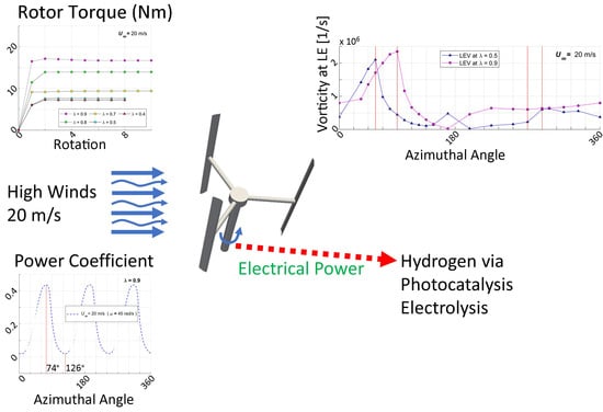
• Much higher torques are delivered at 20m/s, versus the ones produced at 8m/s. Nonetheless, high wind speeds showed just a moderate influence on the final average power coefficient value of a 3-bladed H-Darrieus VAWT. The overall gains are lessened by the increased turbulence and vorticity, which reduce the energy extraction by the rotor during the wind turbine operation, within the same range of tip speed ratios. This matter may require further studies.
• The torque is significantly reduced for blade azimuthal angles θ > 90°. This even yielded negative torque values, which are attributed to flow separation and strong vorticity interactions with the blades.
• The flow vorticity has a noticeable relation with the turbine performance. The leading edge vorticity (LEV) increases until the blade rotation reaches the azimuthal angle of maximum torque. The proposed vorticity index (VI) displays a constant value around 4 before reaching this maximum torque.
• The VI can be used to quantitatively assess vortex separation conditions. After the maximum torque azimuthal position, VI starts decreasing rapidly until minimum values reached because of vortex generation at the LE of the blade and vorticity accumulation at its TE. Furthermore, when the VI attains a value of 1, the Imminent Vortex Separation Condition (IVSC) takes place with the vortex formed by dynamic stall condition almost detaching from the LE of the blade. This occurs at comparable azimuthal angles for equal tip speed ratios, with this being independent of the wind speed.

References

1. Zayats, I. The historical aspect of windmills architectural forms transformation. Procedia Eng. 2015, 117, 685–695. [Google Scholar] [CrossRef] [Green Version]
2. BP plc. bp Energy Outlook 2022 Edition. 2022. Available online: https://www.bp.com/content/dam/bp/business-sites/en/global/corporate/pdfs/energy-economics/energy-outlook/bp-energy-outlook-2022.pdf (accessed on 30 June 2022).
3. Zhao, D.; Han, N.; Goh, E.; Cater, J.; Reinecke, A. Wind Turbines and Aerodynamics Energy Harvesters, 1st ed.; Academic Press: Cambridge, MA, USA, 2019. [Google Scholar]
4. Dai, K.; Bergot, A.; Liang, C.; Xiang, W.-N.; Huang, Z. Environmental issues associated with wind energy—A review. Renew Energy 2015, 75, 911–921. [Google Scholar] [CrossRef]
5. Maalouly, M.; Souaiby, M.; ElCheikh, A.; Issa, J.; Elkhoury, M. Transient analysis of H-type Vertical Axis Wind Turbines using CFD. Energy Rep. 2022, 8, 4570–4588. [Google Scholar] [CrossRef]
6. He, J.; Jin, X.; Xie, S.; Cao, L.; Wang, Y.; Lin, Y.; Wang, N. CFD modeling of varying complexity for aerodynamic analysis of H-vertical axis wind turbines. Renew Energy 2020, 145, 2658–2670. [Google Scholar] [CrossRef]
7. Hossain, M.; Ali, M.H. Future research directions for the wind turbine generator system. Renew. Sustain. Energy Rev. 2015, 49, 481–489. [Google Scholar] [CrossRef]
8. Al-Sharafi, A.; Sahin, A.Z.; Ayar, T.; Yilbas, B.S. Techno-economic analysis and optimization of solar and wind energy systems for power generation and hydrogen production in Saudi Arabia. Renew. Sustain. Energy Rev. 2017, 69, 33–49. [Google Scholar] [CrossRef]
9. Aiche-Hamane, L.; Belhamel, M.; Benyoucef, B.; Hamane, M. Feasibility study of hydrogen production from wind power in the region of Ghardaia. Int. J. Hydrogen Energy 2009, 34, 4947–4952. [Google Scholar] [CrossRef]
10. Benghanem, M.; Mellit, A.; Almohamadi, H.; Haddad, S.; Chettibi, N.; Alanazi, A.M.; Dasalla, D.; Alzahrani, A. Hydrogen Production Methods Based on Solar and Wind Energy: A Review. Energies 2023, 16, 757. [Google Scholar] [CrossRef]
11. Etemadeasl, V.; Esmaelnajad, R.; Dizaji, F.F.; Farzaneh, B. A novel configuration for improving the aerodynamic performance of Savonius rotors. Proc. Inst. Mech. Eng. Part A J. Power Energy 2019, 233, 751–761. [Google Scholar] [CrossRef]
12. Borg, M.; Shires, A.; Collu, M. Offshore floating vertical axis wind turbines, dynamics modelling state of the art. part I: Aerodynamics. Renew. Sustain. Energy Rev. 2014, 39, 1214–1225. [Google Scholar] [CrossRef] [Green Version]
13. Schubel, P.J.; Crossley, R.J. Wind turbine blade design. Energies 2012, 5, 3425–3449. [Google Scholar] [CrossRef] [Green Version]
14. Souaissa, K.; Ghiss, M.; Chrigui, M.; Bentaher, H.; Maalej, A. A comprehensive analysis of aerodynamic flow around H-Darrieus rotor with camber-bladed profile. Wind Eng. 2019, 43, 459–475. [Google Scholar] [CrossRef]
15. Ferreira, C.J.S.; Bijl, H.; Van Bussel, G.; Van Kuik, G. Simulating Dynamic Stall in a 2D VAWT: Modeling strategy, verification and validation with Particle Image Velocimetry data. J. Phys. Conf. Ser. 2007, 75, 012023. [Google Scholar] [CrossRef] [Green Version]
16. Sridhar, S.; Zuber, M.; Shenoy B., S.; Kumar, A.; Ng, E.Y.K.; Radhakrishnan, J. Aerodynamic comparison of slotted and non-slotted diffuser casings for Diffuser Augmented Wind Turbines (DAWT). Renew. Sustain. Energy Rev. 2022, 161, 112316. [Google Scholar] [CrossRef]
17. Rezaeiha, A.; Montazeri, H.; Blocken, B. On the accuracy of turbulence models for CFD simulations of vertical axis wind turbines. Energy 2019, 180, 838–857. [Google Scholar] [CrossRef]
18. Kanyako, F.; Janajreh, I. Vertical Axis Wind Turbine performance prediction for low wind speed environment. In Proceedings of the 2014 IEEE Innovations in Technology Conference, Warwick, RI, USA, 16 May 2014. [Google Scholar] [CrossRef]
19. Lanzafame, R.; Mauro, S.; Messina, M. 2D CFD modeling of H-Darrieus Wind Turbines using a transition turbulence model. Energy Procedia 2014, 45, 131–140. [Google Scholar] [CrossRef] [Green Version]
20. Balduzzi, F.; Bianchini, A.; Maleci, R.; Ferrara, G.; Ferrari, L. Critical issues in the CFD simulation of Darrieus wind turbines. Renew Energy 2016, 85, 419–435. [Google Scholar] [CrossRef]
21. Michna, J.; Rogowski, K. Numerical Study of the Effect of the Reynolds Number and the Turbulence Intensity on the Performance of the NACA 0018 Airfoil at the Low Reynolds Number Regime. Processes 2022, 10, 1004. [Google Scholar] [CrossRef]
22. Elkhoury, M.; Kiwata, T.; Aoun, E. Experimental and numerical investigation of a three-dimensional vertical-axis wind turbine with variable-pitch. J. Wind Eng. Ind. Aerodyn. 2015, 139, 111–123. [Google Scholar] [CrossRef]
23. EMöllerström, E.; Gipe, P.; Beurskens, J.; Ottermo, F. A historical review of vertical axis wind turbines rated 100 kW and above. Renew. Sustain. Energy Rev. 2019, 105, 1–13. [Google Scholar] [CrossRef]
24. Mohamed, O.S.; Ibrahim, A.A.; Etman, A.K.; Abdelfatah, A.A.; Elbaz, A.M. Numerical investigation of Darrieus wind turbine with slotted airfoil blades. Energy Convers. Manag. X 2020, 5, 100026. [Google Scholar] [CrossRef]
25. Ahmedov, A.; Ebrahimi, K.M. Numerical Modelling of an H-type Darrieus Wind Turbine Performance under Turbulent Wind. Am. J. Energy Res. 2017, 5, 63–78. [Google Scholar] [CrossRef]
26. Trivellato, F.; Castelli, M.R. On the Courant-Friedrichs-Lewy criterion of rotating grids in 2D vertical-axis wind turbine analysis. Renew Energy 2014, 62, 53–62. [Google Scholar] [CrossRef]
27. Nguyen, M.T.; Balduzzi, F.; Bianchini, A.; Ferrara, G.; Goude, A. Evaluation of the unsteady aerodynamic forces acting on a vertical-axis turbine by means of numerical simulations and open site experiments. J. Wind. Eng. Ind. Aerodyn. 2020, 198, 104093. [Google Scholar] [CrossRef]
28. Alaimo, A.; Esposito, A.; Messineo, A.; Orlando, C.; Tumino, D. 3D CFD analysis of a vertical axis wind turbine. Energies 2015, 8, 3013–3033. [Google Scholar] [CrossRef] [Green Version]
29. Orlandi, A.; Collu, M.; Zanforlin, S.; Shires, A. 3D URANS analysis of a vertical axis wind turbine in skewed flows. J. Wind Eng. Ind. Aerodyn. 2015, 147, 77–84. [Google Scholar] [CrossRef] [Green Version]
30. Lam, H.; Peng, H. Study of wake characteristics of a vertical axis wind turbine by two- and three-dimensional computational fluid dynamics simulations. Renew Energy 2016, 90, 386–398. [Google Scholar] [CrossRef]
31. Hosseini, A.; Goudarzi, N. Design and CFD study of a hybrid vertical-axis wind turbine by employing a combined Bach-type and H-Darrieus rotor systems. Energy Convers. Manag. 2019, 189, 49–59. [Google Scholar] [CrossRef]
32. Lee, J.-H.; Lee, Y.-T.; Lim, H.-C. Effect of twist angle on the performance of Savonius wind turbine. Renew Energy 2016, 89, 231–244. [Google Scholar] [CrossRef]
33. Alfonsi, G. Reynolds-averaged Navier-Stokes equations for turbulence modeling. Appl. Mech. Rev. 2009, 62, 040802. [Google Scholar] [CrossRef]
34. Geng, F.; Kalkman, I.; Suiker, A.; Blocken, B. Sensitivity analysis of airfoil aerodynamics during pitching motion at a Reynolds number of 1.35×10⁵. J. Wind Eng. Ind. Aerodyn. 2018, 183, 315–332. [Google Scholar] [CrossRef]
35. Ghasemian, M.; Ashrafi, Z.N.; Sedaghat, A. A review on computational fluid dynamic simulation techniques for Darrieus vertical axis wind turbines. Energy Convers. Manag. 2017, 149, 87–100. [Google Scholar] [CrossRef]
36. Barnes, A.; Marshall-Cross, D.; Hughes, B.R. Validation and comparison of turbulence models for predicting wakes of vertical axis wind turbines. J. Ocean Eng. Mar. Energy 2021, 7, 339–362. [Google Scholar] [CrossRef]
37. Ma, N.; Lei, H.; Han, Z.; Zhou, D.; Bao, Y.; Zhang, K.; Zhou, L.; Chen, C. Airfoil optimization to improve power performance of a high-solidity vertical axis wind turbine at a moderate tip speed ratio. Energy 2018, 150, 236–252. [Google Scholar] [CrossRef]
38. ANSYS Inc. ANSYS Fluent Theory Guide 15; ANSYS, Inc.: Canonsburg, PA, USA, 2013. [Google Scholar]
39. Celik, Y.; Ma, L.; Ingham, D.; Pourkashanian, M. Aerodynamic investigation of the start-up process of H-type vertical axis wind turbines using CFD. J. Wind. Eng. Ind. Aerodyn. 2020, 204, 104252. [Google Scholar] [CrossRef]
40. Song, C.; Wu, G.; Zhu, W.; Zhang, X.; Zhao, J. Numerical investigation on the effects of airfoil leading edge radius on the aerodynamic performance of H-rotor Darrieus vertical axis wind turbine. Energies 2019, 12, 3794. [Google Scholar] [CrossRef] [Green Version]
41. AlQurashi, F.; Mohamed, M.H. Aerodynamic forces affecting the H-rotor darrieus wind turbine. Model. Simul. Eng. 2020, 2020, 1368369. [Google Scholar] [CrossRef]
42. Laneville, A.; Vittecoq, P. Dynamic Stall: The Case of the Vertical Axis Wind Turbine. J. Sol. Energy Eng. 1986, 108, 140–145. Available online: http://solarenergyengineering.asmedigitalcollection.asme.org/ (accessed on 9 July 2022). [CrossRef]
43. Dessoky, A.; Bangga, G.; Lutz, T.; Krämer, E. Aerodynamic and aeroacoustic performance assessment of H-rotor darrieus VAWT equipped with wind-lens technology. Energy 2019, 175, 76–97. [Google Scholar] [CrossRef]
44. Choudhry, A.; Arjomandi, M.; Kelso, R. Methods to control dynamic stall for wind turbine applications. Renew Energy 2016, 86, 26–37. [Google Scholar] [CrossRef]
45. Li, S.; Zhang, L.; Yang, K.; Xu, J.; Li, X. Aerodynamic performance of wind turbine airfoil DU 91-W2-250 under dynamic stall. Appl. Sci. 2018, 8, 1111. [Google Scholar] [CrossRef] [Green Version]
46. Menter, F.R. Best Practice: Scale-Resolving Simulations in ANSYS CFD. 2015. Available online: www.ansys.com (accessed on 29 October 2022).
Figure 1. Studies Concerning Wind Turbines in the 1970–2020 Period (2021 Scopus’s Database).
Processes 11 00644 g001
Figure 2. Schematic View of the H-Darrieus Wind Turbine Geometry Used for CFD Calculations.
Processes 11 00644 g002
Figure 3. Description of the Computational Domain and Boundary Conditions Used for Calculations.
Processes 11 00644 g003
Figure 4. Medium Mesh Detailed Grids: (a) Grids in the Entire Computational Domain, (b) Grids in the Rotating Domain, (c) Grids around Blade 1.
Processes 11 00644 g004
Figure 5. Power Coefficient Changes with the Number of Rotations for U = 8 m/s when adopting Different Δ α at λ = 1.
Processes 11 00644 g005
Figure 6. Power Coefficient Changes with Tip Speed Ratio for U = 8 m/s. (o) 2D Model Used in the Present Study, (Δ) 3D Data from [37], (□) Experimental Data from [37].
Processes 11 00644 g006
Figure 7. Average Rotor Overall Torque at Different λ for (a)   U = 8 m/s and (b)   U = 20 m/s, Using the 2D Model of the Present Study. Note: Rotor Average Torque = 1 2 π 0 2 π T   d θ .
Processes 11 00644 g007
Figure 8. Wind and Blades Velocity Components with Forces acting on H-Darrieus’ blades at Various Azimuthal Positions, with FL, and FD representing the lift and drag forces vectors and W and V a representing the relative flow velocity and the induced velocity of wind.
Processes 11 00644 g008
Figure 9. Drag Force for Blades 1, 2 and 3 at Various Azimuthal Angles, for U = 8 m/s at (a) λ = 0.5 and (b) λ = 0.9, Using the 2D Model of the Present Study.
Processes 11 00644 g009
Figure 10. Lift Force for Blades 1, 2 and 3 at Various Azimuthal Angles, for U = 8 m/s at (a) λ = 0.5 and (b) λ = 0.9, Using the 2D Model of the Present Study.
Processes 11 00644 g010
Figure 11. Drag Force for Blade 1at Various Azimuthal Angles, for U = 8 m/s and U = 20 m/s at: (a) λ = 0.5 and (b) λ = 0.9, Using the 2D Model of the Present Study.
Processes 11 00644 g011
Figure 12. Lift Forces for Blade 1at Various Azimuthal Angles, for U = 8 m/s and U = 20 m/s at: (a) λ = 0.5 and (b) λ = 0.9, Using the 2D Model of the Present Study. Note: The direction of the lift forces is established using as a reference the vertical “y” axis.
Processes 11 00644 g012
Figure 13. Torque on Blades 1, 2 and 3 at Various Azimuthal Angles, for U = 8 m/s at: (a) λ = 0.5 and (b) λ = 0.9, Using the 2D Model of the Present Study.
Processes 11 00644 g013
Figure 14. Torque on Blade 1 at Various Azimuthal Angles, for U = 8 m/s and U = 20 m/s at: (a) λ = 0.5 and (b) λ = 0.9, Using the 2D Model of the Present Study.
Processes 11 00644 g014
Figure 15. Power Coefficient Changes with Azimuthal Angles for U = 8 m/s and U = 20 m/s at: (a) λ = 0.5 and (b) λ = 0.9, Using the 2D Model of the Present Study.
Processes 11 00644 g015
Figure 16. Vorticity Values at the LE and TE of Blade 1 at λ =0.5 for (a1a5) U = 8 m/s and (b1b5) U = 20 m/s.
Processes 11 00644 g016aProcesses 11 00644 g016b
Figure 17. LE Vorticity and VI Values for Blade 1 at Various Azimuthal Angles for U = 8 m/s at λ =0.5 and λ =0.9.
Processes 11 00644 g017
Figure 18. LE Vorticity and VI Values for Blade 1 at Various Azimuthal Angles for U = 20 m/s at λ =0.5 and λ =0.9.
Processes 11 00644 g018
Figure 19. Torque and VI for Blade 1 with Azimuthal Position for U = 8 m/s and U = 20 m/s at: (a) λ = 0.5 and (b) λ = 0.9, Using the 2D Model of the Present Study.
Processes 11 00644 g019
Figure 20. Drag Force and VI for Blade 1 with Azimuthal Position for U = 8 m/s and U = 20 m/s at: (a) λ = 0.5 and (b) λ = 0.9, Using the 2D Model of the Present Study.
Processes 11 00644 g020
Figure 21. Lift Force and VI for Blade 1 and VI with Azimuthal Position for U = 8 m/s and U = 20 m/s at: (a) λ = 0.5 and (b) λ = 0.9, Using the 2D Model of the Present Study.
Processes 11 00644 g021
Figure 22. Vorticity Contours for Imminent Vortex Separation Condition (IVSC) for U = 8 m/s and for U = 20 m/s, at (ad) λ = 0.5 and (e,f) λ = 0.9.
Processes 11 00644 g022