Evaluating Industry 4.0 Manufacturing Configurations: An Entropy-Based Grey Relational Analysis Approach

Abstract

Worldwide manufacturing and service sectors are choosing to transform the existing manufacturing sector, particularly reconfigurable manufacturing systems using the technologies of the next generation Industry 4.0. In order to satisfy the demands of the fourth industrial revolution, model evaluation and assessing various candidate configurations in reconfigurable manufacturing systems was developed. The proposed model considers evolving consumer demands and evaluates manufacturing configurations using a gray relational approach. For the case at hand, it is evident that considering all possible dynamic market scenarios 1 to 6, the current manufacturing configuration, i.e., alternative 1, has 89% utilization, total 475 h of earliness and 185 h of lateness in the order demand delivery to the market, and a total of 248 throughput hours and around 1143 bottleneck hours. The main challenge is to make a perfect match between the market demands, variations in product geometry, manufacturing processes and several reconfiguration strategies/alternatives. Furthermore, it is evident that alternative 1 should be reconfigured and that alternative 3 is the best choice. Alternative 3 exhibits 86% system utilization, a total of 926 h of earliness and 521 h of lateness in the order demand delivery to the market, and a total of 127 throughput hours and around 853 bottleneck hours. A simulation framework is used to demonstrate the efficacy of each possible reconfigurable production setup. The sensitivity analysis is also carried out by adjusting the weights through principal component analysis and validating the acquired ranking order. Thus, if the decision makers want to provide a preference to all criteria, the order of the choices of configurations is found to be alternative 3, alternative 1, alternative 4, alternative 2 and alternative 5.

1. Introduction

Industry 4.0 represents a significant advancement in the incorporation of information technology into the manufacturing process. It creates an opportunity for improving the production process’ flexibility, speed, efficiency and quality; pursues new business models, manufacturing techniques and other innovations; and allows for a different level of mass customization [1]. In a published report, an international consultant stated that countries with a relative unavailability of industrial tradition can be seen as a positive advantage, providing an opportunity to step directly to the fourth industrial revolution [2]. Saudi Arabia’s policymakers, for example, have eagerly grasped the idea of Industry 4.0, as it presents a roadmap for a future which very much in line with the requirements of the economic growth plan (Vision 2030) [2]. The major transformation projects in Saudi Arabia are tailored to the policies of Industry 4.0. These ventures concentrate on artificial intelligence, robotics and a semi-autonomous environment for service and manufacturing.

The modern concept of digitization and technological change is having an immense impact on manufacturing industries. The current manufacturing setup has begun to transform for the future industrial revolution (Industry 4.0). This industrial revolution [3,4,5,6] is about collecting, exchanging and/or sharing digitized information through the supply chain of consumers, service providers, suppliers and manufacturers. Industry 4.0 also includes a roadmap and develops strategies to deal with the optimal use of collected digital data in decision making. For example, Siemens [7], one of the stakeholders in Industry 4.0, has invested heavily (accounting for 75% of its value chain) in automated machines and computers for its electronics business. Siemens demands are captured and controlled by using a digital product code and are directly communicated to their own assembly plants as well as being communicated in parallel to the suppliers and their service providers. The performance and effectiveness of a supply chain or system involving manufacturers, suppliers and service providers is influenced by multiple factors, namely market demand, production rate, operation management planning, scheduling, flexibility, automation level, etc. Based on these factors, the manufacturing systems can be classified as machine center systems (MCSs), cellular manufacturing systems (CMSs), flexible manufacturing systems (FMSs), agile manufacturing systems (AMSs) and reconfigurable manufacturing systems (RMSs), etc.

These are the manufacturing systems that have been adopted in recent times to conceive the idea of Industry 4.0 [8]. A common MCS is the computer numeric control machine center system, where the positioning and feeding of tools, products, fixtures and or pallets is automatically performed, while robots or advanced mechanized automated systems perform loading and unloading [9]. Moreover, based on the concept of group technology, a fixed CMS is created to carry out the manufacturing of a certain set of product families [10]. The FMS is designed for a specific group of a product family; however, it is highly automated in terms of transportation, distribution and production flexibility [11]. AMS is designed to share a common database related to customer demands and organization facilities, and to create strategies to respond quickly to dynamic market/customer needs [12]. RMS is different from cellular, agile and FMSs. RMS focuses on personalized flexibility rather than manufacturing flexibility [13]. RMS is a collection of reconfigurable-machine centers, tools, and inspection and material handling systems. However, as the most advanced system, RMSs are the closest to Industry 4.0 [14]. Figure 1 highlights the evolution of manufacturing concepts and manufacturing systems in different eras of industrial revolutions.

The capabilities of both FMSs and specialized manufacturing systems (DMSs) are included in RMSs, which combine computer-based technologies (such as intelligent sensors, autonomous robots, automatic material handling, computer-based machines, etc.) with manufacturing systems. At the start of the fourth industrial revolution, the manufacturing sector is utilizing cutting-edge technologies including the Internet of Things, cloud computing, virtual reality, simulation, blockchain, big data, additive manufacturing, etc., which are powerful drivers for RMSs to meet the demands of competitive markets [15,16,17,18]. For dynamic markets, the manufacturing of ordered products is dependent on the organization’s manufacturing system’s capability. In such scenario, it is desired by the organization to have a cost-effective framework for the production method whenever adapting to perform repeated adjustments that are needed from time to time [19,20]. Therefore, the RMS is the nearest to Industry 4.0 [21]. It lowers system costs by implementing the production system for the entire part family and offers the requisite versatility to manufacture all the products/components in the part family. Similarly, having extensively used the internet, computational and analysis tools, Industry 4.0 can implement new adaptive manufacturing processes, such as 3D printing, and offer to push customize goods according to specific demands and priorities [22]. These advanced manufacturing solutions [23], which include a collection of autonomous, collaborative industrial robots and a group of modular production systems dominated by integrated sensors and standardized interfaces, are among the enabling technologies that will define the coming industrial revolution. This adds value to the growth of the future factories, which are called smart factories. These factories evolve to the complex environment and utilize manufacturing systems that are easily reconfigurable [24]. The researchers [25] also indicate that the revolutionary technologies promoted by the philosophy of Industry 4.0, including big data analysis and real-time collection, versatile transportation networks or remote and collaborative robotics, can make a major contribution toward enhancing the configurability of manufacturing systems.

One of the prerequisites of Industry 4.0, managing changes and uncertainties in dynamic demand situations, is something that the RMS specializes in and allows system designers to dynamically organize development processes and transform the system over time. On other hand, a limitation with the RMS is the determination of the most appropriate configuration from the array of alternatives available. With the advent of Industry 4.0 technologies, the number of alternative manufacturing configurations has further increased. Certainly, in an unpredictable business setting of Industry 4.0, it is important to select and implement the most appropriate configuration from the set of accessible possibilities [26,27,28]. There are several variables that may affect the choice of a given appropriate production configuration, and researchers [21,29] defined several performance metrics, namely cost, reliability, usage and efficiency, to have a responsive RMS. These performance parameters can be very valuable in finding the optimum configuration from the pool of existing configurations. Researchers explored the RMS in order to plan its production operations [21], and to pick the reconfigurable candidate machines [30]. Their key goal was to minimize the total cost (sum of production, reconfiguration, and alteration of tools and cost of tools) and the overall completion time. Similarly, researchers [31] focused to improve the design of production cells and the deployment of automated material handling systems. Further researchers addressed the volatile market requirements through the integration of emerging manufacturing cells, where, depending on the product demand, the cells were built with the reconfiguration approach [32]. In order to have the manufacturing cells and scheduling of part families in the RMS, an artificial neural network [33] and a tabu search algorithm [34] were used. As stated by Singh et al. [21], there are major challenges in selecting the most feasible configuration, especially in the environment of Industry 4.0. A wide variety of alternative configurations are available, rendering the selection process a complicated and tedious activity. Therefore, the evaluation and selection of an alternate configuration are the focus of extensive research in field of RMSs [30]. Thus, to evaluate a wide range of configurations and choose the optimal one, a structured methodology is needed. The most popular and often used method for selecting candidates for industrial applications is multi-criteria decision making (MCDM) [35,36]. Over recent years, many MCDM approaches have been established to support in choosing and justifying the best choice. For example, the analytic hierarchy process [37], technique for order of preferences by similarity to ideal solution [38], elimination and choice translating reality [39], preference ranking organization method for enrichment evaluation [40], grey relational analysis [41], fuzzy approaches [42], etc., have been used. Researchers considered the ecological and environmental capacities for an interregional transfer of polluting industries [43]. Similarly, from an empirical data standpoint, one can establish that an environmental supervision path under collaboration by governments at different levels offers implications for achieving green innovation and optimizing pollution emission mechanisms [44]. Researchers adopted the MCDM approach in the decision making of a green and water-saving development in agriculture [45].

All MCDM evaluation models need multi-criteria preference decision analysis and evaluation over the available alternatives. Each alternative configuration has a different physical structure, and each performance criterion has a different objective. Thus, finding the appropriate weight for each criterion is one of the important issues that needs to be addressed. Numerous methods are available in the literature and most of them are grouped into two groups: subjective and objective weights. Commonly, operation managers adopt the decision maker’s expertise and judgment and prefer subjective weights; however, in the era of Industry 4.0, the use of objective weight is more useful. The objective weights method makes use of mathematical models, for example, principal component analysis [46] and entropy analysis [47].

It is evident from the published literature that most manufacturing companies invest in advanced manufacturing systems as they feel that the existing procedures, processes and technology are insufficient to satisfy the current or potential demands [48]. Companies do not see the advantage of committing to one particular product, especially in a dynamic market that is more open and competitive: where users/buyers are aware of and have better choices. Although, in the longer term, these manufacturing organizations need to be smart enough to develop their production systems intelligently enough to learn how to create things faster to keep pace with the anticipated demand, and to continue to overcome severe decision-making challenges. The fluctuating market demand mainly includes variations in product geometry and manufacturing constraints. Among the several existing strategies, the reconfigurable manufacturing system (RMS) is the choice, owing to its numerous benefits for Industry 4.0. This work aims to conduct a study for analyzing and ranking various potential configurations in reconfigurable manufacturing systems. The goal is to provide an evaluation framework for alternative manufacturing configurations to meet the fourth industrial revolution. A simulation approach is used to demonstrate the efficiency of each feasible production configuration. In this work, an entropy-based grey relational formulation is applied to analyze different configurations and select the most suitable one based on the customers’ preferences. The research discussed here considers the changes in the market demand, including product varieties, and enacts an objective approach focusing on entropy weight coupled with grey relational analysis. The sensitivity analysis is also performed by deriving the different weights through principal component analysis and justifying the ranking order acquired with entropy weight coupled grey relational analysis.

Here, the objective is to apply an entropy-based grey relational formulation to examine the different manufacturing configurations and identify the most appropriate configuration depending on the dynamic market requirements. The research described here considers variations in the market demand as well as product varieties and proposes an evaluation approach focusing on entropy weight coupled with grey relational analysis. By modifying the weights through principal component analysis and validating the ranking order, the sensitivity analysis is also carried out. Entropy and grey relational analysis have an advantage over other methods since they are capable of handling a number of multiple criteria and alternatives. They are extremely effective mathematical tools for the modelling and control of uncertain systems, and they provide a stable and adaptable framework for dealing with challenging decision-making issues. The paper is organized into five sections. Section 2 presents the adopted research methodology and case study on hand. Section 3 presents the adopted entropy-based grey relational approach to propose a suitable manufacturing system in response to Industry 4.0′s dynamic market demand. Section 4 presents managerial points of discussion. Finally, this paper is concluded in Section 5 and outlines future research scopes.

2. Research Methodology and the Problem on Hand

In the context of the Industry 4.0 environment, due to unpredictable demands from customers, it is important to evaluate and rank many possible configurations to find the most suitable manufacturing configuration. As the research method, initially alternate manufacturing configurations, performance criteria and scenarios are set. Subsequently, future market demand scenarios in terms of product variations, product shape, material and manufacturing complexity are assessed. Afterwards, a determination of whether there is a need to reconfigure the current configuration is performed. If the response is affirmative, which alternative production arrangement is the best choice? To resolve this issue, an evaluation model that aids decision makers in identifying the most suitable manufacturing configuration that delivers Industry 4.0 capabilities is developed. Here, the challenge is to make a perfect match between the market demand, variations in product geometry, manufacturing processes and several reconfiguration strategies/alternatives. Thus, different criterion weighting methods are proposed and are later used in the development of the evaluation model that aids decision makers and provides an insight into the comparative analysis. The details are presented below, as well as in the following section.

In this study, the evaluation model that aids decision makers in identifying the most suitable manufacturing configuration and delivers Industry 4.0 capabilities is presented. In this evaluation model, alternative manufacturing configurations (i ϵ (1 to m)), performance criterions (j ϵ (1 to n)) and scenarios (k ϵ (1 to s)) are considered. For example, for a given market scenario k, and for an alternative manufacturing system 1, X_11k is the measure of performance criterion 1, and weightage is assigned to performance criterion 1 (expressed as W_1k). The structure of the derived decision matrix for market scenario k, for all alternative manufacturing configurations (i ϵ (1 to m)), is as presented in

Table 1. Decision matrix for Industry 4.0 market ‘scenario k’.

Performance Criterion (j) → Alternative (i) ↓	1	2	…	n
1	X11k	X12k	…	X1nk
2	X21k	X22k	…	X2nk
.	.	.	…	.
m	Xm1k	Xm2k	…	Xmnk
Criterion weight →	W1k	W2k	…	Wnk

below.

In order to adjust variation in the market demand and product variety, the management of manufacturing organizations is interested in developing and implementing reconfiguration strategies in the Industry 4.0 framework. For the case at hand, there are two levels of future market demand, either low demand or high demand, in comparison to present market situation. However, for product varieties, that is a variation in terms of product shape, material and manufacturing complexity, in which there are three levels, i.e., low, medium and high variation (refer to

Table 2. The alternative manufacturing configurations (six different market scenarios) and their evaluation based on five performance criteria.

Market Scenario: k	Alternative: i	Performance Criteria: j
		Performance Criterion 1	Performance Criterion 2	Performance Criterion 3	Performance Criterion 4	Performance Criterion 5
Market Scenario: 1 Market Demand: High Product Variety: Low	Alternative: 1	X111 = 87.72	X121 = 236.25	X131 = 325.38	X141 = 27.11	X151 = 545.04
	Alternative: 2	X211 = 84.60	X221 = 416.82	X231 = 211.72	X241 = 103.85	X251 = 374.15
	Alternative: 3	X311 = 86.21	X321 = 566.62	X331 = 156.73	X341 = 194.53	X351 = 521.10
	Alternative: 4	X411 = 65.01	X421 = 509.64	X431 = 186.90	X441 = 161.59	X451 = 469.28
	Alternative: 5	X511 = 61.94	X521 = 445.11	X531 = 208.25	X541 = 117.40	X551 = 391.36
Market Scenario: 2 Market Demand: Low Product Variety: Low	Alternative: 1	X112 = 64.79	X122 = 183.38	X132= 376.58	X142 = 15.36	X152 = 406.30
	Alternative: 2	X212 = 70.24	X222 = 274.68	X232= 304.50	X242 = 45.70	X252 = 239.77
	Alternative: 3	X312 = 77.06	X322 = 360.64	X332= 254.39	X342 = 78.30	X352 = 315.98
	Alternative: 4	X412 = 63.26	X422 = 331.99	X432= 272.72	X442 = 59.80	X452 = 297.91
	Alternative: 5	X512 = 60.32	X522 = 300.54	X532 = 287.77	X542 = 42.39	X552 = 266.17
Market Scenario: 3 Market Demand: High Product Variety: Medium	Alternative: 1	X113 = 92.93	X123 = 692.41	X133 = 157.22	X143 = 301.51	X153 = 1690.42
	Alternative: 2	X213 = 89.31	X223 = 1132.45	X233 = 116.65	X243 = 711.53	X253 = 1084.61
	Alternative: 3	X313 = 90.14	X323= 1534.96	X333 = 81.53	X343 = 718.11	X353 = 1297.11
	Alternative: 4	X413 = 69.84	X423= 1160.99	X433 = 115.04	X443 = 727.81	X453 = 1113.32
	Alternative: 5	X513 = 71.04	X523 = 1059.74	X533 = 117.77	X543 = 628.13	X553 = 963.02
Market Scenario: 4 Market Demand: Low Product Variety: Medium	Alternative: 1	X114= 80.21	X124= 266.73	X134 = 314.28	X144 = 25.08	X154 = 620.56
	Alternative: 2	X214 = 81.78	X224 = 464.44	X234 = 215.22	X244 = 136.70	X254 = 432.62
	Alternative: 3	X314 = 83.60	X324 = 574.05	X334 = 183.76	X344 = 207.47	X354 = 528.20
	Alternative: 4	X414 = 67.45	X424 = 495.62	X434 = 217.26	X444 = 156.69	X454 = 462.08
	Alternative: 5	X514 = 64.93	X524 = 449.30	X534 = 230.45	X544 = 122.52	X554 = 395.75
Market Scenario: 5 Market Demand: Low Product Variety: High	Alternative: 1	X115 = 96.78	X125 = 1162.72	X135 = 73.79	X145 = 700.89	X155 = 2871.57
	Alternative: 2	X215 = 88.44	X225 = 1676.26	X235 = 58.29	X245 = 1208.01	X255 = 1543.52
	Alternative: 3	X315 = 89.64	X325 = 1993.89	X335 = 44.00	X345 = 1511.55	X355 = 1807.63
	Alternative: 4	X415 = 66.93	X425 = 1746.08	X435 = 56.78	X445 = 1266.71	X455 = 1641.52
	Alternative: 5	X515 = 67.31	X525 = 1621.92	X535 = 56.14	X545 = 1140.46	X555 = 1394.66
Market Scenario: 6 Market Demand: High Product Variety: High	Alternative: 1	X116 = 93.93	X126 = 711.83	X136 = 123.62	X146 = 300.14	X156 = 1728.41
	Alternative: 2	X216 = 84.71	X226 = 1056.70	X236 = 85.51	X246 = 617.61	X256 = 1008.13
	Alternative: 3	X316 = 87.28	X326 = 1287.48	X336 = 64.56	X346 = 824.13	X356 = 1221.62
	Alternative: 4	X416 = 65.59	X426 = 1149.35	X436 = 91.50	X446 = 704.92	X456 = 1085.18
	Alternative: 5	X516 = 61.68	X526 = 1061.38	X536 = 88.10	X546 = 612.57	X556 = 931.75

Criterion 1: percentage manufacturing configuration utilization (objective: the larger the better). Criterion 2: total hours of earliness in the order demand delivery to the market (objective: the larger the better). Criterion 3: total throughput hours for the provided market demand (objective: the smaller the better). Criterion 4: total hours of lateness in the order demand delivery to the market (objective: the smaller the better). Criterion 5: total bottleneck hours in the order demand delivery to the market (objective: the smaller the better).

). In Table 2, for market scenario-1, product demand is at a low level and variation in the product’s geometry, size and shape of the material, manufacturing complexity, and so on is also at a low level. Moreover, for market scenario-2, the manufacturing plant demand increases to a high level without a change in product varieties. On the contrary, for market scenario-6, the demand of the product rises to a high level and as well as a high level of variation in product geometry, size and shape of the material, manufacturing complexity, and so on. Table 2 presents the alternative manufacturing configurations which have to possibility to execute the above six different market scenarios, and each of the alternatives is evaluated based on five performance criterions. In Table 2 below, alternative 1 is the present configuration with an optimum number of computer-controlled numerical machines and software to satisfy the present market demand and product varieties. In order to apply reconfiguration strategies, one has to develop virtual alternative configurations and product demand scenarios. Alternatives 2 and 3 are machine-based configurations, where a set of machines are replaced by one or more than one advanced reconfigurable machine tool. Alternatives 4 and 5 are cell-based configurations, where the option that is provided is to group and relocate the set of machines. Performance measures of alternative configurations were computed through simulation experiments by establishing different market scenarios. The performance criterion results for five alternative configurations corresponding to market scenarios 1 to 6 are presented in Table 2.

As the objective is to keep pace with the forecasted demand, the challenge is to make a perfect match between the market demand, variations in product geometry, manufacturing processes and several reconfiguration strategies/alternatives. The evaluation of alternative configurations is an attempt to offer an assessment lens to those who look for alternative reconfigurable manufacturing configurations to cater to the manufacturing suited for the fourth industrial revolution. These alternative configurations are analyzed to arrive at a meaningful ranking. The steps involved in the analysis are presented below in Section 3.

3. Adopted Approach and Its Application

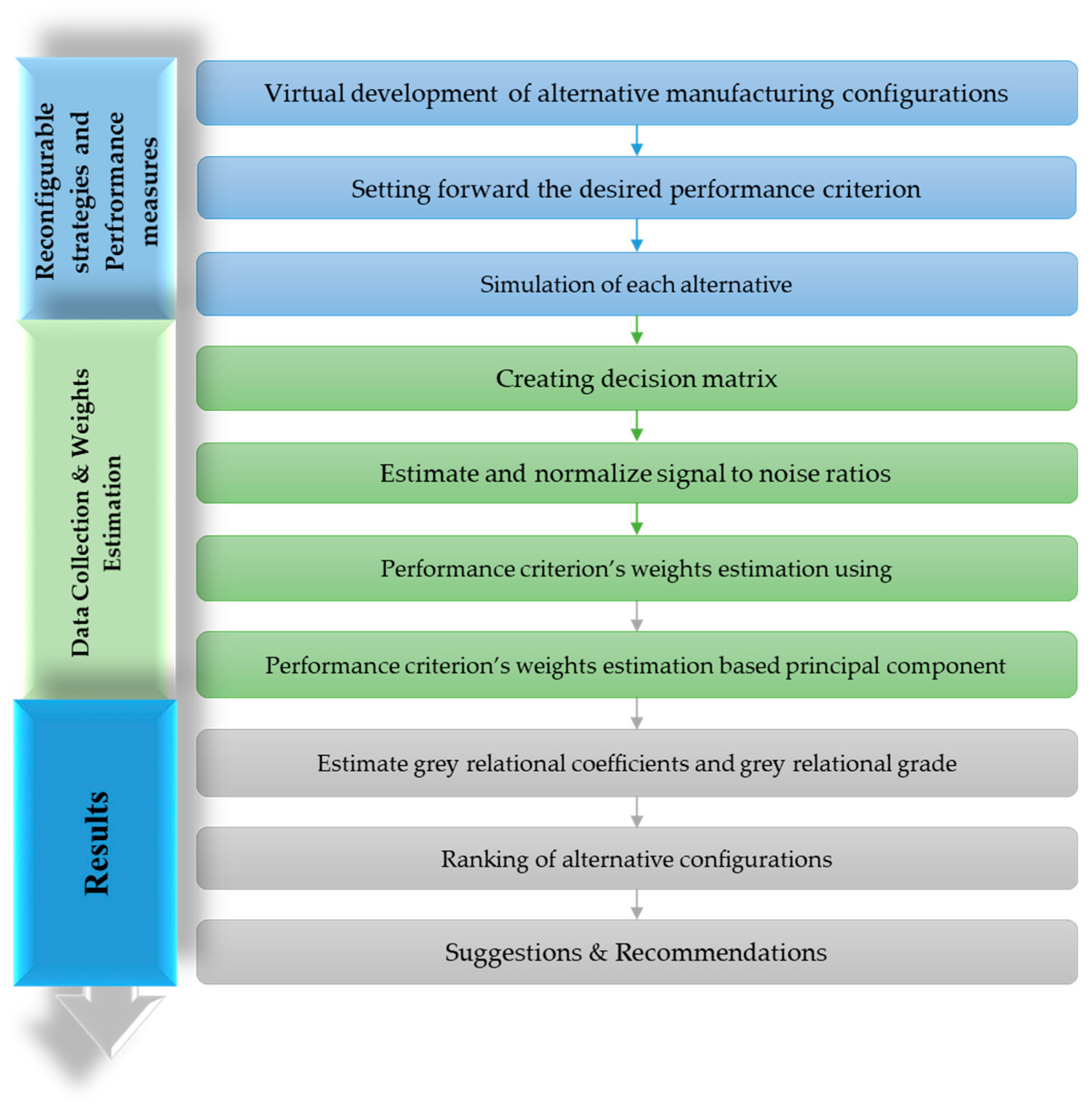
To implement reconfigurable strategies in the Industry 4.0 framework and to meet the dynamic market demands, manufacturing managers try to adjust capacity and functionality and consider alternative manufacturing configurations by combining existing groups of hardware (i.e., machines and tools). They also need to consider many factors, such as virtual development of alternative manufacturing configurations, setting forward the desired performance measures, defining the performance measure weights, simulation of each alternative, and then put forward the best match between market scenarios and alternative configurations. In this approach, alternative manufacturing configurations (i ϵ (1 to m)), performance criterion (j ϵ (1 to n)) and scenario (k ϵ (1 to s)) are considered. Furthermore, X_mnk is the measure of a performance criterion n for an alternative m, for a given market scenario k (refer to Table 1). Refer to Figure 2 for the adopted approach. The steps involved in the adopted approach are presented in the following subsections.

3.1. Estimate and Normalize Signal to Noise Ratios

In order to convert incomparable decision data into comparable data, the decision matrix (refer to Table 2) was analyzed for signal to noise ratios using Minitab. The normalization of signal to noise ratios was performed to convert incomparable data to comparable data. The normalized signal to noise ratio η_ijk for the jth performance criterion and the ith alternative for the kth market scenario is expressed as follows:

$${\mathsf{\eta }}_{\mathrm{i}\mathrm{j}\mathrm{k}}={\left[\frac{{\mathrm{X}}_{\mathrm{ij}}-\underset{\mathrm{i}}{\min }{\mathrm{X}}_{\mathrm{i}\mathrm{j}}}{\underset{\mathrm{i}}{\max }{\mathrm{X}}_{\mathrm{i}\mathrm{j}}-\underset{\mathrm{i}}{\min }{\mathrm{X}}_{\mathrm{i}\mathrm{j}}}\right]}_{\mathrm{k}}$$

(1)

In Equation (1), X_ij is the measure of the performance criterion j for an alternative i, for a given market scenario k. After normalization of all measured performance criteria values for each alternative configuration for a market scenario k, the equation for this is expressed as follows:

$${\mathsf{\eta }}_{\mathrm{i}\mathrm{j}\mathrm{k}}={\left[\begin{array}{cccc}{\mathsf{\eta }}_{11}& {\mathsf{\eta }}_{12}& \dots & {\mathsf{\eta }}_{1\mathrm{n}}\\ :& :& :& :\\ :& :& :& :\\ {\mathsf{\eta }}_{\mathrm{m}1}& {\mathsf{\eta }}_{\mathrm{m}2}& \dots & {\mathsf{\eta }}_{\mathrm{m}\mathrm{n}}\end{array}\right]}_{\mathrm{k}}$$

(2)

For the problem at hand (refer to Section 2), the normalized decision matrices (η_ijk) for all six market scenarios (refer to Table 2) are displayed as follows:

$${\mathsf{\eta }}_{\mathrm{i}\mathrm{j}\mathrm{k}}=\left[\begin{array}{c}{\left[\begin{array}{cccccc}\raisebox{1ex}{$\mathrm{j}\to $}\!\left/ \!\raisebox{-1ex}{$\mathrm{i}\downarrow $}\right.& 1& 2& 3& 4& 5\\ 1& 1& 0& 1& 0& 1\\ 2& 0.8959& 0.649& 0.4117& 0.6815& 0\\ 3& 0.9501& 1& 0& 1& 0.8806\\ 4& 0.139& 0.8788& 0.241& 0.9059& 0.6022\\ 5& 0& 0.7241& 0.3891& 0.7437& 0.1195\end{array}\right]}_{k=1}{\left[\begin{array}{ccccc}0.2919& 0& 1& 0& 1\\ 0.6216& 0.5974& 0.4584& 0.6694& 0\\ 1& 1& 0& 1& 0.5233\\ 0.1943& 0.8776& 0.1774& 0.8345& 0.4117\\ 0& 0.7305& 0.3143& 0.6233& 0.1981\end{array}\right]}_2\\ {\left[\begin{array}{ccccc}1& 0& 1& 0& 1\\ 0.8609& 0.6180& 0.5455& 0.9743& 0.2113\\ 0.8933& 1& 0& 0.9848& 0.5293\\ 0& 0.6492& 0.5243& 1& 0.2578\\ 0.0596& 0.5346& 0.5600& 0.8329& 0\end{array}\right]}_3{\left[\begin{array}{ccccc}0.8362& 0& 1& 0& 1\\ 0.9129& 0.7236& 0.2945& 0.8025& 0.1980\\ 1& 1& 0& 1& 0.6418\\ 0.1507& 0.8083& 0.3121& 0.8671& 0.3445\\ 0& 0.6803& 0.4219& 0.7507& 0\end{array}\right]}_4\\ {\left[\begin{array}{ccccc}1& 0& 1& 0& 1\\ 0.7556& 0.6783& 0.5440& 0.7083& 0.1404\\ 0.7922& 1& 0& 1& 0.3591\\ 0& 0.7539& 0.4932& 0.7710& 0.2257\\ 0.0154& 0.6172& 0.4713& 0.6335& 0\end{array}\right]}_5{\left[\begin{array}{ccccc}1& 0& 1& 0& 1\\ 0.7544& 0.6667& 0.4326& 0.7144& 0.1275\\ 0.8254& 1& 0& 1& 0.4384\\ 0.1461& 0.8085& 0.5368& 0.8453& 0.2467\\ 0& 0.6741& 0.4786& 0.7063& 0\end{array}\right]}_6\end{array}\right]$$

3.2. Estimate Grey Relational Coefficients and Grey Relational Grade

The estimated normalized signal to noise ratios ‘η_ijk’ are further processed to get relational coefficients (i.e., ξ_ijk) for the jth performance characteristic and the ith alternative for the kth scenario, and are expressed as follows:

$${\mathsf{\xi }}_{\mathrm{i}\mathrm{j}\mathrm{k}}={\left[\frac{{\mathrm{m}\mathrm{i}\mathrm{n}}_{\mathrm{j}}{\mathrm{m}\mathrm{i}\mathrm{n}}_{\mathrm{i}}\left|{\mathrm{X}}_{\mathrm{j}}^{\mathrm{o}}-{\mathrm{X}}_{\mathrm{ij}}\right|+\mathsf{\xi }{\max }_{\mathrm{j}}{\max }_{\mathrm{i}}\left|{\mathrm{X}}_{\mathrm{j}}^{\mathrm{o}}-{\mathrm{X}}_{\mathrm{i}\mathrm{j}}\right|}{\left|{\mathrm{X}}_{\mathrm{j}}^{\mathrm{o}}-{\mathrm{X}}_{\mathrm{ij}}\right|+\mathsf{\xi }{\max }_{\mathrm{j}}{\max }_{\mathrm{i}}\left|{\mathrm{X}}_{\mathrm{j}}^{\mathrm{o}}-{\mathrm{X}}_{\mathrm{i}\mathrm{j}}\right|}\right]}_{\mathrm{k}}$$

(3)

In Equation (3), ${\mathrm{X}}_{\mathrm{j}}^{\mathrm{o}}$ is the normalized signal to noise ratio for the jth performance criterion and ξ is the distinguishing coefficient, which is defined in the range of $0\le \mathsf{\xi }\le 1$ and is usually taken as 0.5. Moreover, X_ij is the measure of the performance criterion j for an alternative I and corresponding market scenario k, and the equation for this is expressed as follows:

$${\mathsf{\xi }}_{\mathrm{i}\mathrm{j}\mathrm{k}}={\left[\begin{array}{ccccc}\raisebox{1ex}{$\mathrm{j}\to $}\!\left/ \!\raisebox{-1ex}{$\mathrm{i}\downarrow $}\right.& 1& 2& \dots & \mathrm{n}\\ 1& {\mathsf{\xi }}_{11}& {\mathsf{\xi }}_{12}& \dots & {\mathsf{\xi }}_{1\mathrm{n}}\\ :& :& :& :& :\\ :& :& :& :& :\\ \mathrm{m}& {\mathsf{\xi }}_{\mathrm{m}1}& {\mathsf{\xi }}_{\mathrm{m}2}& \dots & {\mathsf{\xi }}_{\mathrm{m}\mathrm{n}}\end{array}\right]}_{\mathrm{k}}$$

(4)

The relational coefficient matrices (ξ_ijk) for all six market scenarios (refer Table 2) are displayed as follows:

$${\mathsf{\xi }}_{\mathrm{i}\mathrm{j}\mathrm{k}}=\left[\begin{array}{c}{\left[\begin{array}{cccccc}\raisebox{1ex}{$\mathrm{j}\to $}\!\left/ \!\raisebox{-1ex}{$\mathrm{i}\downarrow $}\right.& 1& 2& 3& 4& 5\\ 1& 1& 0.3333& 1& 0.3333& 1\\ 2& 0.8277& 0.5876& 0.4594& 0.6109& 0.3333\\ 3& 0.9093& 1& 0.3333& 1& 0.8072\\ 4& 0.3674& 0.805& 0.3971& 0.8415& 0.5569\\ 5& 0.3333& 0.6444& 0.4501& 0.6612& 0.3622\end{array}\right]}_{\mathrm{k}=1}{\left[\begin{array}{ccccc}0.4139& 0.3333& 1& 0.3333& 1\\ 0.5692& 0.5540& 0.4800& 0.6020& 0.3333\\ 1& 1& 0.3333& 1& 0.5119\\ 0.3829& 0.8034& 0.3780& 0.7513& 0.4594\\ 0.3333& 0.6497& 0.4217& 0.5703& 0.3840\end{array}\right]}_2\\ {\left[\begin{array}{ccccc}1& 0.3333& 1& 0.3333& 1\\ 0.7823& 0.5669& 0.5238& 0.9512& 0.3880\\ 0.8241& 1& 0.3333& 0.9704& 0.5151\\ 0.3333& 0.5877& 0.5125& 1& 0.4025\\ 0.3471& 0.5179& 0.5319& 0.7495& 0.3333\end{array}\right]}_3{\left[\begin{array}{ccccc}0.7532& 0.3333& 1& 0.3333& 1\\ 0.8517& 0.6440& 0.4148& 0.7169& 0.3840\\ 1& 1& 0.3333& 1& 0.5826\\ 0.3706& 0.7229& 0.4209& 0.7901& 0.4327\\ 0.3333& 0.6100& 0.4638& 0.6673& 0.3333\end{array}\right]}_4\\ {\left[\begin{array}{ccccc}1& 0.3333& 1& 0.3333& 1\\ 0.6717& 0.6085& 0.5230& 0.6316& 0.3678\\ 0.7064& 1& 0.3333& 1& 0.4383\\ 0.3333& 0.6702& 0.4966& 0.6850& 0.3924\\ 0.3368& 0.5664& 0.4860& 0.5770& 0.3333\end{array}\right]}_5{\left[\begin{array}{ccccc}1& 0.3333& 1& 0.3333& 1\\ 0.6706& 0.6000& 0.4684& 0.6365& 0.3643\\ 0.7412& 1& 0.3333& 1& 0.4710\\ 0.3693& 0.7231& 0.5191& 0.7637& 0.3989\\ 0.3333& 0.6054& 0.4895& 0.6300& 0.3333\end{array}\right]}_6\end{array}\right]$$

The relational coefficients are still unique for the individual performance criterion, and can be converted to a single, multi-response parameter (ϒ_ik). ϒ_ik is used for ith alternative corresponding to the kth scenario over an n number of performance criteria. The ϒ_ik, which is estimated using ξ_ijk, is a relational coefficient, and W_jk is the performance criterion j with a certain weightage for a given market scenario k. Researchers [46,47] initially proposed a different criterion weighting methods and later developed these methods into a useful statistical tool for analysis. In the absence of a performance criterion’s subjective weights, Shannon’s entropy and principal component analysis [49,50] are among the approaches used for obtaining a performance criterion’s weights for a multi-criteria decision-making scenario. These two techniques were developed as effective analytical tools for the optimization of multi-criteria measures because they are based on statistical approaches, free from subjective judgment, and use original information. The various steps involved in Shannon’s entropy weighting and principal component weighting are described and compared below.

3.3. Performance Criterion’s Weight Estimation

After normalization of all the measured performance criteria values for each alternative configuration for a market scenario k, the normalized decision matrix η_ijk is used to calculate W_jk. The criterion entropy weight value for a given market scenario k is represented as E_jk and calculated by using Equation (5) below.

$${\mathrm{E}}_{\mathrm{j}\mathrm{k}}={\left[-\frac{\sum _{\mathrm{i}=1}^{\mathrm{m}}{\mathrm{F}}_{\mathrm{i}\mathrm{j}}{\ln \mathrm{F}}_{\mathrm{i}\mathrm{j}}}{\ln \mathrm{m}}\right]}_{\mathrm{k}}$$

(5)

In Equation (5), ${\mathrm{F}}_{\mathrm{i}\mathrm{j}\mathrm{k}}=\frac{{\mathsf{\eta }}_{\mathrm{i}\mathrm{j}\mathrm{k}}}{\sum _{\mathrm{i}=1}^{\mathrm{m}}{\mathsf{\eta }}_{\mathrm{i}\mathrm{j}\mathrm{k}}}$ for i ϵ (1 to m); j ϵ (1 to n); and k ϵ (1 to s). For each performance criterion, using the above normalized data (refer to Equation (2)), the entropy indices are calculated using the above Equation (5), and are presented below in a matrix form.

$${\mathrm{E}}_{\mathrm{j}\mathrm{k}}=\begin{array}{c}\left[\begin{array}{cccccc}\raisebox{1ex}{$\mathrm{j}\to $}\!\left/ \!\raisebox{-1ex}{$\mathrm{k}\downarrow $}\right.& 1& 2& 3& 4& 5\\ 1& 0.2618& 0.3901& 0.6683& 0.3548& 0.4171\\ 2& 0.6047& 0.4050& 0.6388& 0.4438& 0.6368\\ 3& 0.2472& 0.6571& 0.6175& 0.1198& 0.6304\\ 4& 0.3218& 0.4152& 0.6757& 0.3202& 0.6042\\ 5& 0.2860& 0.4810& 0.6427& 0.4565& 0.6085\\ 6& 0.4052& 0.4399& 0.6519& 0.3901& 0.6023\end{array}\right]\end{array}$$

The larger the entropy weight of the performance criterion j is, the more important the performance measure is, and the same occurs in a reverse format. Based on the entropy indices, the performance criterion j weightage for a given market scenario k is calculated using Equation (6) below.

$${\mathrm{W}}_{\mathrm{j}\mathrm{k}}=\left[\frac{1-{\mathrm{E}}_{\mathrm{j}\mathrm{k}}}{\mathrm{n}-\sum _{\mathrm{j}=1}^{\mathrm{n}}{\mathrm{E}}_{\mathrm{j}\mathrm{k}}}\right]$$

(6)

In Equation (6), $\sum _{\mathrm{j}=1}^{\mathrm{n}}{\mathrm{W}}_{\mathrm{j}\mathrm{k}}=1$; subsequently, the entropy weights are determined using Equation (6), and using entropy indices ${\mathrm{E}}_{\mathrm{j}\mathrm{k}}$. The estimated entropy weights are presented below in Equation (7).

$${\mathrm{W}}_{\mathrm{j}\mathrm{k}}=\begin{array}{c}\left[\begin{array}{cccccc}\raisebox{1ex}{$\mathrm{j}\to $}\!\left/ \!\raisebox{-1ex}{$\mathrm{k}\downarrow $}\right.& 1& 2& 3& 4& 5\\ 1& 0.2539& 0.2097& 0.1141& 0.2219& 0.2005\\ 2& 0.1741& 0.2620& 0.1591& 0.2449& 0.1599\\ 3& 0.2617& 0.1536& 0.1357& 0.3124& 0.1311\\ 4& 0.2547& 0.2196& 0.1218& 0.2553& 0.1486\\ 5& 0.2827& 0.2055& 0.1415& 0.2152& 0.1550\\ 6& 0.2369& 0.2231& 0.1387& 0.2429& 0.1584\end{array}\right]\end{array}$$

(7)

In Equation (7), it is evident that in the case of the market scenario k = 1, there is a low market demand and a low variation in product variety, and management wish to have a maximum percentage manufacturing configuration utilization, which is evident form the entropy weight calculations. In the case of scenario 1, criterion 1 (i.e., percentage manufacturing configuration utilization) has a maximum entropy weight, and criterion 3 (i.e., total throughput hours for the provided market demand) has a minimum entropy weight with least importance. Thus, for the market scenario 1 to 6, the objective is as follows: ‘is there any need to reconfigure the present configuration (Alternative 1)?’. If the answer is ‘yes’, reconfiguration is needed. In this case, which alternative manufacturing configuration is the best alternative choice? To resolve this issue, the relational coefficients as multi-response parameter ϒ_ik are estimated for ith alternative for a given kth market scenario over an n number of performance criteria (refer to Section 3.4 for details).

Similarly, as an alternative approach, principal component-based criterion weights are estimated and explained below. In this approach, which uses the ${\mathsf{\eta }}_{\mathrm{i}\mathrm{j}\mathrm{k}}$ normalized decision matrix (refer to Equations (1)–(3)), a covariance matrix (CM) is generated for each market scenario k using Equation (8).

$${\mathrm{C}\mathrm{M}}_{\mathrm{k}}={\left(\frac{\mathrm{C}\mathrm{o}\mathrm{v}\left({\mathsf{\eta }}_{\mathrm{i}\left(\mathrm{j}\right),}{\mathsf{\eta }}_{\mathrm{i}\left(\mathrm{l}\right)}\right)}{{\mathsf{\sigma }}_{\left({\mathsf{\eta }}_{\mathrm{i}\left(\mathrm{j}\right)}\right)}\ast {\mathsf{\sigma }}_{\left({\mathsf{\eta }}_{\mathrm{i}\left(\mathrm{l}\right)}\right)}}\right)}_{\mathrm{k}}$$

(8)

In Equation (8), $\mathrm{C}\mathrm{o}\mathrm{v}\left({\mathsf{\eta }}_{\mathrm{i}\left(\mathrm{j}\right),}{\mathsf{\eta }}_{\mathrm{i}\left(\mathrm{l}\right)}\right)$ is the covariance of sequences ${\mathsf{\eta }}_{\mathrm{i}\left(\mathrm{j}\right)},{\mathsf{\eta }}_{\mathrm{i}\left(\mathrm{l}\right)};{\mathsf{\sigma }}_{\left({\mathsf{\eta }}_{\mathrm{i}\left(\mathrm{j}\right)}\right)}$ is the standard deviation of sequence ${\mathsf{\eta }}_{\mathrm{i}\left(\mathrm{j}\right)}$; ${\mathsf{\sigma }}_{\left({\mathsf{\eta }}_{\mathrm{i}\left(\mathrm{l}\right)}\right)}$ is the standard deviation of sequence ${\mathsf{\eta }}_{\mathrm{i}\left(\mathrm{l}\right)}$ for a given market scenario k, where, i ϵ (1 to m); j ϵ (1 to n); and k ϵ (1 to s). After having a normalized decision matrix for a given market scenario k, the covariance matrix is obtained using Equation (9) and the outcome is presented below.

$${\mathrm{C}\mathrm{M}}_{\mathrm{k}}={\left[{\mathsf{\eta }}_{\mathrm{i}\mathrm{j}\mathrm{k}}\right]}^{\mathrm{T}}\ast \left[{\mathsf{\eta }}_{\mathrm{i}\mathrm{j}\mathrm{k}}\right]={\left[\begin{array}{cccc}{\mathsf{\eta }}_{11}& {\mathsf{\eta }}_{21}& \dots & {\mathsf{\eta }}_{\mathrm{m}1}\\ {\mathsf{\eta }}_{12}& {\mathsf{\eta }}_{22}& :& {\mathsf{\eta }}_{\mathrm{m}2}\\ :& :& :& :\\ {\mathsf{\eta }}_{1\mathrm{n}}& {\mathsf{\eta }}_{2\mathrm{n}}& \dots & {\mathsf{\eta }}_{\mathrm{m}\mathrm{n}}\end{array}\right]}_{\mathrm{k}}\ast {\left[\begin{array}{cccc}{\mathsf{\eta }}_{11}& {\mathsf{\eta }}_{12}& \dots & {\mathsf{\eta }}_{1\mathrm{n}}\\ {\mathsf{\eta }}_{21}& {\mathsf{\eta }}_{22}& :& {\mathsf{\eta }}_{2\mathrm{n}}\\ :& :& :& :\\ {\mathsf{\eta }}_{\mathrm{m}1}& {\mathsf{\eta }}_{\mathrm{m}2}& \dots & {\mathsf{\eta }}_{\mathrm{m}\mathrm{n}}\end{array}\right]}_{\mathrm{k}}$$

(9)

$${\mathrm{C}\mathrm{M}}_{\mathrm{k}}={\left[\begin{array}{cccc}\mathrm{c}\mathrm{o}\mathrm{v}\left(\mathrm{11,11}\right)& \mathrm{c}\mathrm{o}\mathrm{v}\left(\mathrm{11,12}\right)& \dots & \mathrm{c}\mathrm{o}\mathrm{v}\left(\mathrm{11,1}\mathrm{n}\right)\\ \mathrm{c}\mathrm{o}\mathrm{v}\left(\mathrm{12,11}\right)& \mathrm{c}\mathrm{o}\mathrm{v}\left(\mathrm{12,12}\right)& :& \mathrm{c}\mathrm{o}\mathrm{v}\left(\mathrm{12,1}\mathrm{n}\right)\\ :& :& :& :\\ \mathrm{c}\mathrm{o}\mathrm{v}(1\mathrm{n},11)& \mathrm{c}\mathrm{o}\mathrm{v}(1\mathrm{n},12)& \dots & \mathrm{c}\mathrm{o}\mathrm{v}(1\mathrm{n},1\mathrm{n})\end{array}\right]}_{\mathrm{k}}$$

$${\mathrm{C}\mathrm{M}}_{\mathrm{k}}=\left[\begin{array}{c}{\left[\begin{array}{cccccc}\raisebox{1ex}{$\mathrm{j}\to $}\!\left/ \!\raisebox{-1ex}{$\mathrm{i}\downarrow $}\right.& 1& 2& 3& 4& 5\\ 1& 0.2357& -0.0719& 0.1458& -0.0755& 0.0917\\ 2& & 0.1507& -0.1418& 0.1526& -0.0490\\ 3& & & 0.1363& -0.1430& 0.0322\\ 4& & & & 0.1547& -0.0547\\ 5& & & & & 0.1955\end{array}\right]}_{k=1}\\ {\left[\begin{array}{ccccc}0.1552& 0.0476& -0.0527& 0.0650& -0.0010\\ & 0.1514& -0.1478& 0.1457& -0.0846\\ & & 0.1450& -0.1422& 0.0758\\ & & & 0.1443& -0.0860\\ & & & & \end{array}\right]}_2\\ {\left[\begin{array}{ccccc}0.2398& -0.0299& 0.0058& -0.0915& 0.1325\\ & 0.1298& -0.1242& 0.1391& -0.0731\\ & & 0.1257& -0.1181& 0.0498\\ & & & 0.1842& -0.1327\\ & & & & 0.1481\end{array}\right]}_3\\ {\left[\begin{array}{ccccc}0.2184& -0.0201& -0.0061& -0.0301& 0.1110\\ & 0.1440& -0.1377& 0.1487& -0.0849\\ & & 0.1348& -0.1410& 0.0699\\ & & & 0.1549& -0.0987\\ & & & & 0.1539\end{array}\right]}_4\\ {\left[\begin{array}{ccccc}0.2212& -0.0632& 0.0331& -0.0645& 0.1265\\ & 0.1374& -0.1246& 0.1385& -0.1069\\ & & 0.1257& -0.1244& 0.0805\\ & & & 0.1398& -0.1103\\ & & & & 0.1511\end{array}\right]}_5\\ {\left[\begin{array}{ccccc}0.1964& -0.0676& 0.0175& -0.0732& 0.1265\\ & 0.1422& -0.1242& 0.1447& -0.0147\\ & & 0.1265& -0.1246& 0.0750\\ & & & 0.1476& -0.115\\ & & & & 0.1531\end{array}\right]}_6\end{array}\right]$$

The calculated covariance matrix is further processed to find eigenvalues and eigenvectors. The eigenvalues and eigenvectors are determined from the covariance matrix (CM) (refer to Equation (10)).

$${({\mathrm{C}\mathrm{M}}_{\mathrm{k}}-\mathsf{\lambda }}_{\mathrm{j}}{\mathrm{I}}_{\mathrm{m}}){\mathrm{V}}_{\mathrm{j}\mathrm{k}}=0$$

(10)

In Equation (10), ${\mathrm{C}\mathrm{M}}_{\mathrm{k}}$ is correlation matrix ${\mathsf{\lambda }}_{\mathrm{j},}{\sum }_{\mathrm{j}=1}^{\mathrm{n}}{\mathsf{\lambda }}_{\mathrm{j}}=\mathrm{n}$ are eigenvalues; ${\mathrm{V}}_{\mathrm{i}\mathrm{j}\mathrm{k}}={[{\mathrm{a}}_{\mathrm{k}1},{\mathrm{a}}_{\mathrm{k}2},{\mathrm{a}}_{\mathrm{k}3}\dots ..{\mathrm{a}}_{\mathrm{k}\mathrm{n}}]}^{\mathrm{T}}$ are eigenvectors corresponding to the eigenvalues ${\mathsf{\lambda }}_{\mathrm{j}}$. The estimated eigenvalues and eigenvectors are as presented below.

$${\mathsf{\lambda }}_{\mathrm{j}}=\left[\begin{array}{cccccc}\mathrm{k}\downarrow & 1\mathrm{s}\mathrm{t}& 2\mathrm{n}\mathrm{d}& 3\mathrm{r}\mathrm{d}& 4\mathrm{t}\mathrm{h}& 5\mathrm{t}\mathrm{h}\\ 1& 0.5267& 0.2262& 0.1237& 0.0003& 0.0000\\ 2& 0.5169& 0.1516& 0.0697& 0.0008& 0.0000\\ 3& 0.5169& 0.1516& 0.0697& 0.0008& 0.0000\\ 4& 0.5109& 0.2541& 0.0407& 0.0003& 0.0000\\ 5& 0.5465& 0.1929& 0.0303& 0.0000& 0.0055\\ 6& 0.5468& 0.1855& 0.0281& 0.0053& 0.0000\end{array}\right]$$

$${\mathrm{V}}_{\mathrm{j}\mathrm{k}}=\left[\begin{array}{c}{\left[\begin{array}{cccccc}\mathrm{j}\downarrow & 1\mathrm{s}\mathrm{t} \mathrm{P}\mathrm{r}\mathrm{i}\mathrm{n}\mathrm{c}\mathrm{i}\mathrm{p}\mathrm{a}\mathrm{l} \mathrm{c}\mathrm{o}\mathrm{m}\mathrm{p}\mathrm{o}\mathrm{n}\mathrm{e}\mathrm{n}\mathrm{t} \left(\mathrm{P}\mathrm{C}\right)& 2\mathrm{n}\mathrm{d} \mathrm{P}\mathrm{C}& 3\mathrm{r}\mathrm{d} \mathrm{P}\mathrm{C}& 4\mathrm{t}\mathrm{h} \mathrm{P}\mathrm{C}& 5\mathrm{t}\mathrm{h} \mathrm{P}\mathrm{C}\\ 1& -0.4288& 0.6139& 0.6580& 0.0759& 0.0223\\ 2& 0.5002& 0.2892& 0.0109& 0.1570& 0.8009\\ 3& -0.4461& -0.3706& -0.0428& 0.7702& 0.2620\\ 4& 0.5115& 0.2721& 0.0270& 0.6117& -0.5380\\ 5& -0.3245& 0.5728& -0.7512& 0.0470& -0.0032\end{array}\right]}_{\mathrm{k}=1}\\ {\left[\begin{array}{cccccc}\mathrm{j}\downarrow & 1\mathrm{s}\mathrm{t} \mathrm{P}\mathrm{r}\mathrm{i}\mathrm{n}\mathrm{c}\mathrm{i}\mathrm{p}\mathrm{a}\mathrm{l} \mathrm{c}\mathrm{o}\mathrm{m}\mathrm{p}\mathrm{o}\mathrm{n}\mathrm{e}\mathrm{n}\mathrm{t}& 2\mathrm{n}\mathrm{d} \mathrm{P}\mathrm{C}& 3\mathrm{r}\mathrm{d} \mathrm{P}\mathrm{C}& 4\mathrm{t}\mathrm{h} \mathrm{P}\mathrm{C}& 5\mathrm{t}\mathrm{h} \mathrm{P}\mathrm{C}\\ 1& -0.2403& -0.8608& -0.4324& -0.1061& 0.0547\\ 2& -0.5294& 0.0727& 0.2865& -0.1568& 0.7796\\ 3& 0.5159& -0.0137& -0.3198& 0.5446& 0.5787\\ 4& -0.5256& -0.0242& 0.119& 0.8102& -0.2328\\ 5& 0.3459& -0.5029& 0.7849& 0.1052& 0.0146\end{array}\right]}_{\mathrm{k}=2}\\ {\left[\begin{array}{cccccc}\mathrm{j}\downarrow & 1\mathrm{s}\mathrm{t} \mathrm{P}\mathrm{r}\mathrm{i}\mathrm{n}\mathrm{c}\mathrm{i}\mathrm{p}\mathrm{a}\mathrm{l} \mathrm{c}\mathrm{o}\mathrm{m}\mathrm{p}\mathrm{o}\mathrm{n}\mathrm{e}\mathrm{n}\mathrm{t}& 2\mathrm{n}\mathrm{d} \mathrm{P}\mathrm{C}& 3\mathrm{r}\mathrm{d} \mathrm{P}\mathrm{C}& 4\mathrm{t}\mathrm{h} \mathrm{P}\mathrm{C}& 5\mathrm{t}\mathrm{h} \mathrm{P}\mathrm{C}\\ 1& -0.2403& -0.8608& -0.4324& -0.1061& 0.0547\\ 2& -0.5294& 0.0727& 0.2865& -0.1568& 0.7796\\ 3& 0.5159& -0.0137& -0.3198& 0.5446& 0.5787\\ 4& -0.5256& -0.0242& 0.119& 0.8102& -0.2328\\ 5& 0.3459& -0.5029& 0.7849& 0.1052& 0.0146\end{array}\right]}_{\mathrm{k}=3}\\ {\left[\begin{array}{cccccc}\mathrm{j}\downarrow & 1\mathrm{s}\mathrm{t} \mathrm{P}\mathrm{r}\mathrm{i}\mathrm{n}\mathrm{c}\mathrm{i}\mathrm{p}\mathrm{a}\mathrm{l} \mathrm{c}\mathrm{o}\mathrm{m}\mathrm{p}\mathrm{o}\mathrm{n}\mathrm{e}\mathrm{n}\mathrm{t}& 2\mathrm{n}\mathrm{d} \mathrm{P}\mathrm{C}& 3\mathrm{r}\mathrm{d} \mathrm{P}\mathrm{C}& 4\mathrm{t}\mathrm{h} \mathrm{P}\mathrm{C}& 5\mathrm{t}\mathrm{h} \mathrm{P}\mathrm{C}\\ 1& -0.2447& 0.8381& -0.4783& 0.0772& 0.0548\\ 2& 0.5036& 0.2213& 0.2215& -0.0054& 0.8052\\ 3& -0.4614& -0.3134& -0.1521& 0.6989& 0.4221\\ 4& 0.5342& 0.1825& 0.1137& 0.7068& -0.4109\\ 5& -0.4339& 0.3422& 0.8284& 0.0773& -0.0499\end{array}\right]}_{\mathrm{k}=4}\\ {\left[\begin{array}{cccccc}\mathrm{j}\downarrow & 1\mathrm{s}\mathrm{t} \mathrm{P}\mathrm{r}\mathrm{i}\mathrm{n}\mathrm{c}\mathrm{i}\mathrm{p}\mathrm{a}\mathrm{l} \mathrm{c}\mathrm{o}\mathrm{m}\mathrm{p}\mathrm{o}\mathrm{n}\mathrm{e}\mathrm{n}\mathrm{t}& 2\mathrm{n}\mathrm{d} \mathrm{P}\mathrm{C}& 3\mathrm{r}\mathrm{d} \mathrm{P}\mathrm{C}& 4\mathrm{t}\mathrm{h} \mathrm{P}\mathrm{C}& 5\mathrm{t}\mathrm{h} \mathrm{P}\mathrm{C}\\ 1& 0.4091& -0.8017& 0.4356& 0.0099& 0.0033\\ 2& -0.4696& -0.2852& -0.1033& 0.7231& 0.4057\\ 3& 0.4024& 0.3976& 0.3472& 0.0489& 0.7463\\ 4& -0.4762& -0.2752& -0.0472& -0.6884& 0.4705\\ 5& 0.4727& -0.2051& -0.8227& -0.0254& 0.2388\end{array}\right]}_{\mathrm{k}=5}\\ {\left[\begin{array}{cccccc}\mathrm{j}\downarrow & 1\mathrm{s}\mathrm{t} \mathrm{P}\mathrm{r}\mathrm{i}\mathrm{n}\mathrm{c}\mathrm{i}\mathrm{p}\mathrm{a}\mathrm{l} \mathrm{c}\mathrm{o}\mathrm{m}\mathrm{p}\mathrm{o}\mathrm{n}\mathrm{e}\mathrm{n}\mathrm{t}& 2\mathrm{n}\mathrm{d} \mathrm{P}\mathrm{C}& 3\mathrm{r}\mathrm{d} \mathrm{P}\mathrm{C}& 4\mathrm{t}\mathrm{h} \mathrm{P}\mathrm{C}& 5\mathrm{t}\mathrm{h} \mathrm{P}\mathrm{C}\\ 1& 0.3854& -0.7667& 0.4565& -0.2334& 0.0289\\ 2& -0.4830& -0.2592& -0.2408& -0.3266& 0.7313\\ 3& 0.3897& 0.4647& 0.0424& -0.7896& 0.0834\\ 4& -0.4978& -0.2341& -0.1675& -0.4637& -0.6740\\ 5& 0.4674& -0.2726& -0.8389& 0.0194& -0.0554\end{array}\right]}_{\mathrm{k}=6}\end{array}\right]$$

The eigenvectors, or principal components, are used to find the performance criterion’s weight. The principal component Y_mk is formulated and presented in Equation (11) that follows. The square of principal components gives the performance criterion weight W_jk for a given market scenario k.

$${{\mathrm{W}}_{\mathrm{j}\mathrm{k}}=(\mathrm{Y}}_{\mathrm{m}\mathrm{k}}{)}^2=({\sum }_{\mathrm{j}=1}^{\mathrm{n}}{\mathrm{X}}_{\mathrm{m}}\left(\mathrm{j}\right).{\mathrm{V}}_{\mathrm{j}\mathrm{k}}{)}^2$$

(11)

In above Equation (11), $\sum _{\mathrm{j}=1}^{\mathrm{n}}{\mathrm{W}}_{\mathrm{j}\mathrm{k}}=1$ and k ϵ (1 to s), and the estimated principal components-based criteria weights are presented below.

$${\mathrm{W}}_{\mathrm{j}\mathrm{k}}=\left[\begin{array}{cccccc}\raisebox{1ex}{$\mathrm{j}\to $}\!\left/ \!\raisebox{-1ex}{$\mathrm{k}\downarrow $}\right.& 1& 2& 3& 4& 5\\ 1& 0.1839& 0.2502& 0.1990& 0.2616& 0.1053\\ 2& 0.0577& 0.2803& 0.2662& 0.2763& 0.1196\\ 3& 0.1818& 0.1699& 0.1209& 0.3164& 0.2110\\ 4& 0.0599& 0.2536& 0.2129& 0.2854& 0.1883\\ 5& 0.1674& 0.2205& 0.1619& 0.2268& 0.2234\\ 6& 0.1485& 0.2333& 0.1519& 0.2478& 0.2185\end{array}\right]$$

(12)

From Equation (12), it is evident that in the case of market scenario k = 1, there is a low market demand and a low variation in product variety, and management wish to minimize lateness in delivering orders, which is evident form the principal component weight calculations. In the case of scenario 1, criterion 1 (i.e., percentage manufacturing configuration utilization) has a 18.39% weight, and criterion 3 (i.e., the total throughput hours for the given market demand) has a 19.9% weight with least importance of 10.53% to bottleneck. Thus, the goal of market scenario k (1to 6) is to determine whether there is a need to reconfigure the current configuration (i.e., alternative 1). If the response is affirmative, which alternative production arrangement is the best choice? To resolve this issue, the relational coefficients, as multi-response parameter ϒ_ik, are estimated for ith alternative for a given kth market scenario over an n number of performance criteria (refer to Section 3.4 below).

3.4. Ranking of Alternative Configurations for Industry 4.0

The relational coefficients, as multi-response parameter ϒ_ik, are estimated using Equation (13). The highest ϒ_ik provides the best alternative choice for the kth market scenario.

$${\mathrm{\Upsilon }}_{\mathrm{i}\mathrm{k}}=\sum _{\mathrm{j}=1}^{\mathrm{n}}{\mathrm{W}}_{\mathrm{j}\mathrm{k}}{\mathsf{\xi }}_{\mathrm{i}\mathrm{j}\mathrm{k}}$$

(13)

For a given market scenario, the multiplication of respective entropy weights (refer Equations (6) and (7)) with relational coefficients ξ_ijk is performed to obtain the value for a given market scenario, and the corresponding alternative relational grade values. The calculated relational grade values and ranks are based on entropy-based criterion weights (refer to Equations (14) and (15)).

$${\mathrm{\Upsilon }}_{\mathrm{i}\mathrm{k}}=\left[\begin{array}{cccccc}\raisebox{1ex}{$\mathrm{i}\to $}\!\left/ \!\raisebox{-1ex}{$\mathrm{k}\downarrow $}\right.& 1& 2& 3& 4& 5\\ 1& 0.1425& 0.1176& 0.1725& 0.1212& 0.0981\\ 2& 0.1120& 0.1043& 0.1632& 0.1189& 0.0993\\ 3& 0.1378& 0.1430& 0.1579& 0.1228& 0.1045\\ 4& 0.1241& 0.1298& 0.1714& 0.1141& 0.0990\\ 5& 0.1439& 0.1164& 0.1471& 0.1021& 0.0975\\ 6& 0.1379& 0.1140& 0.1525& 0.1139& 0.0975\end{array}\right]$$

(14)

$$~\mathrm{R}\mathrm{a}\mathrm{n}\mathrm{k}\left[\begin{array}{cccccc}\raisebox{1ex}{$\mathrm{i}\to $}\!\left/ \!\raisebox{-1ex}{$\mathrm{k}\downarrow $}\right.& 1& 2& 3& 4& 5\\ 1& 2& 4& 1& 3& 5\\ 2& 3& 4& 1& 2& 5\\ 3& 3& 2& 1& 4& 5\\ 4& 3& 2& 1& 4& 5\\ 5& 2& 3& 1& 4& 5\\ 6& 2& 3& 1& 4& 5\end{array}\right]$$

(15)

From the relational grade (${\mathrm{\Upsilon }}_{\mathrm{i}\mathrm{k}}$), it is evident that the present manufacturing configuration should be reconfigured and the alternative 3 with the highest rank is the best suitable choice for all six scenarios. Similarly, for all given market scenarios, the multiplication of the respective principal component-based criteria weights W_jk with relational coefficients ξ_ijk is performed to obtain relational grade values, and alternatives are ranked in a descending order (refer to Equations (16) and (17)).

$${\mathrm{\Upsilon }}_{\mathrm{i}\mathrm{k}}=\left[\begin{array}{cccccc}\raisebox{1ex}{$\mathrm{i}\to $}\!\left/ \!\raisebox{-1ex}{$\mathrm{k}\downarrow $}\right.& 1& 2& 3& 4& 5\\ 1& 0.1318& 0.1171& 0.1661& 0.1254& 0.1046\\ 2& 0.1190& 0.1044& 0.1528& 0.1221& 0.1034\\ 3& 0.1352& 0.1369& 0.1552& 0.1248& 0.1046\\ 4& 0.1252& 0.1159& 0.1559& 0.1204& 0.1053\\ 5& 0.1404& 0.1113& 0.1435& 0.1054& 0.0931\\ 6& 0.1358& 0.1096& 0.1489& 0.1158& 0.0988\end{array}\right]$$

(16)

$$~\mathrm{R}\mathrm{a}\mathrm{n}\mathrm{k}\left[\begin{array}{cccccc}\raisebox{1ex}{$\mathrm{i}\to $}\!\left/ \!\raisebox{-1ex}{$\mathrm{k}\downarrow $}\right.& 1& 2& 3& 4& 5\\ 1& 2& 4& 1& 3& 5\\ 2& 3& 4& 1& 2& 5\\ 3& 3& 2& 1& 4& 5\\ 4& 2& 4& 1& 3& 5\\ 5& 2& 3& 1& 4& 5\\ 6& 2& 4& 1& 3& 5\end{array}\right]$$

(17)

From the relational grade rank ${\mathrm{\Upsilon }}_{ik}$, it is evident that the present manufacturing configuration should be reconfigured and the alternative 3 with the highest rank is the best suitable choice for all six scenarios, which are summarized in

Table 3. Set of weights and the ranking order of alternate configurations.

Set of Weights	Rankings of Alternative Configurations for Each Scenarios
	Scenario:1 #					Scenario:2					Scenario:3					Scenario:4					Scenario:5					Scenario:6
	Alternative: 1	Alternative: 2	Alternative: 3	Alternative: 4	Alternative: 5	Alternative: 1	Alternative: 2	Alternative: 3	Alternative: 4	Alternative: 5	Alternative: 1	Alternative: 2	Alternative: 3	Alternative: 4	Alternative: 5	Alternative: 1	Alternative: 2	Alternative: 3	Alternative: 4	Alternative: 5	Alternative: 1	Alternative: 2	Alternative: 3	Alternative: 4	Alternative: 5	Alternative: 1	Alternative: 2	Alternative: 3	Alternative: 4	Alternative: 5
Set 1: equal weights for all performance measures	2	4	1	3	5	3	4	1	2	5	3	2	1	4	5	2	4	1	3	5	2	3	1	4	5	2	4	1	3	5
Set 2: entropy weight	2	4	1	3	5	3	4	1	2	5	3	2	1	4	5	3	2	1	4	5	2	3	1	4	5	2	3	1	4	5
Set 3: principal component weight	2	4	1	3	5	3	4	1	2	5	3	2	1	4	5	2	4	1	3	5	2	3	1	4	5	2	4	1	3	5

^# Six different market scenarios (refer to Table 2).

.

4. Discussion

The present manufacturing configuration is alternative 1, with an optimum number of computer-controlled numerical machines and software to satisfy the present market demand and product varieties. Virtual alternative configurations, such as alternatives 2 and 3 are machine-based configurations, and alternatives 4 and 5 are cell-based configurations, are set in order to apply a reconfiguration strategy in context of Industry 4.0. The performance criterion results for five alternative configurations corresponding to market scenarios 1 to 6 are obtained using simulation tools. As and when there is a low market demand and a low variation in product variety, management wish to have a maximum utilization of the configuration, while least importance is provided to the total throughput hours. However, when the demand is high, management set to maximize earliness to deliver the demand as early as possible, while least importance is provided to system utilization. Thus, for the market scenario 1 to 6, the objective is depicted as follows: ‘is there any need to reconfigure the present configuration (alternative 1)?’. If the answer is ‘yes’, that reconfiguration is needed. In this case, which alternative manufacturing configuration is the best alternative choice? In order to address this problem, principal component-based criterion weights and entropy weights are used to estimate the grey relational coefficients as a multi-response parameter for sensitivity and comparison analysis. Thus, as the market demand falls to a low level and product variety also drops down (refer to Table 2), the manufacturing configuration alternative 3 is the best choice, followed by the current configuration alternative 1 (refer to Table 3). Moreover, in the future, when the market demand rises to a high level and product variety remains low (i.e., scenario 2), the manufacturing configuration alternative 3 remains the best choice, followed by configuration alternatives 4, 1, 2 and 5, in that order. Similarly, when the market demand is low and the product variety is medium or high (see scenarios 3 and 5), alternative manufacturing configuration 3 outperforms alternative configurations 2, 1, 4 and 5. Finally, when the market demand and the product variety rises to a high level, configuration 3 performs very well in terms of all performance measures. According to the gray relational performance weightage approach, it is evident that the present manufacturing configuration should be reconfigured, and that the alternative 3 is the best choice suitable for all six scenarios, which are summarized in Table 3. The recommendation of this research is to implement the potential of Industry 4.0-integrated manufacturing systems to improve the reconfiguration capabilities of the current manufacturing systems. This research should concentrate on the development of dynamic reconfiguration strategies that utilize real-time data to optimize production processes and adapt to the ever-changing dynamic demand of manufacturing.

5. Conclusions

The majority of industrial businesses are investing in modern production technologies. They believe that present methods, techniques and technologies are insufficient to meet the current and or projected demands. This results in the reconfiguration of industrial systems as a strategy for production and operation management. However, any change without previous appraisal is risky. In such instances, the options must often be assessed using various performance factors. Industry 4.0 was interested in restructuring its current manufacturing configuration to meet dynamic market circumstances, as depicted above. Decision makers state that several performance factors need to be taken into consideration while evaluating alternatives. The industry managers’ performance goals for the case at hand included increasing system utilization, minimizing total cycle time, increasing on-time deliveries, minimizing delivery delays, and minimizing the amount of time that products had to wait before being processed, inspected and moved. To assess production configurations, a multi-criteria decision-making gray relational analysis technique was applied. The alternative configurations were designed to function under various demand and operational circumstances. For example, for market scenario 1, which is characterized by high demand and low product variety, it is clear that the current manufacturing system, referred to as alternative 1, achieves a utilization rate of 88%. As the market demand decreases to a low level with a corresponding decrease in product variety, the utilization rate of alternative configuration 1 drops to 64%. Conversely, when the product variety increases to a medium level, the utilization rate of alternative configuration 1 rises to 92%. With a decrease in the market demand, the percentage utilization of the current arrangement, i.e., alternative configuration 1, drops to 80%. Regarding market scenarios 1 and 3 and performance criterion system utilization, it is clear that alternative 1 excels in comparison to the other alternatives. Similarly, for market scenario 1, the average overall leading time to deliver the requested demand to the market is 236.25 h for alternative 1. In contrast, under the same market conditions, the alternative configuration 3 delivers the ordered demand to the market 566.62 h earlier than the due time. For all market scenarios 1 to 6 (refer to Table 2), it is evident that alternative 3 outperforms all other alternatives.

It was revealed that there is a need to reconfigure the present manufacturing configuration in response to the dynamic demand to stay competitive in the market. By assessing alternative configurations using a grey relational approach, decision makers decided to reconfigure their present manufacturing configuration. However, the reconfiguration choice set was reduced to a machine-based reconfiguration of alternative 3. There is a need to bring the cost and risk associated with reconfigurations into this presented approach as a future scope. Another interesting aspect could be the development of a model to incorporate real-time criteria for manufacturing system reconfigurations.

During the reconfiguration process, optimization models and algorithms can minimize downtime, save costs, maximize resource use and improving efficiency and production. Implementing any changes, however, is constrained because reconfiguring production systems can disturb current workflows and processes. To achieve a smooth transition and reduce employee opposition, effective change management tactics are needed. In order to improve the agility, responsiveness and adaptability of manufacturing systems, further research should aim to concentrate on creating sophisticated reconfiguration techniques in an Industry 4.0 environment that make use of emerging technologies, such as edge computing, block chain and 5G.

References

- Spenhoff, P.; Wortmann, J.C.; Semini, M. EPEC 4.0: An Industry 4.0-Supported Lean Production Control Concept for the Semi-Process Industry. Prod. Plan. Control 2022, 33, 1337–1354. [Google Scholar] [CrossRef]
- A.T. Kearney Man Sees Future of Saudi Arabia in 3-D Vision|Arab News. Available online: https://www.arabnews.com/node/1319326/business-economy (accessed on 23 August 2023).
- Pech, M.; Vrchota, J. The Product Customization Process in Relation to Industry 4.0 and Digitalization. Processes 2022, 10, 539. [Google Scholar] [CrossRef]
- Mourtzis, D.; Angelopoulos, J.; Panopoulos, N. A Literature Review of the Challenges and Opportunities of the Transition from Industry 4.0 to Society 5.0. Energies 2022, 15, 6276. [Google Scholar] [CrossRef]
- Konstantinidis, F.K.; Myrillas, N.; Mouroutsos, S.G.; Koulouriotis, D.; Gasteratos, A. Assessment of Industry 4.0 for Modern Manufacturing Ecosystem: A Systematic Survey of Surveys. Machines 2022, 10, 746. [Google Scholar] [CrossRef]
- Hallioui, A.; Herrou, B.; Santos, R.S.; Katina, P.F.; Egbue, O. Systems-Based Approach to Contemporary Business Management: An Enabler of Business Sustainability in a Context of Industry 4.0, Circular Economy, Competitiveness and Diverse Stakeholders. J. Clean. Prod. 2022, 373, 133819. [Google Scholar] [CrossRef]
- Petrisor, I.; Cozmiuc, D. Global Supply Chain Management Organization at Siemens in the Advent of Industry 4.0. Available online: https://www.igi-global.com/chapter/global-supply-chain-management-organization-at-siemens-in-the-advent-of-industry-40/www.igi-global.com/chapter/global-supply-chain-management-organization-at-siemens-in-the-advent-of-industry-40/239318 (accessed on 19 March 2023).
- Leng, J.; Wang, D.; Shen, W.; Li, X.; Liu, Q.; Chen, X. Digital Twins-Based Smart Manufacturing System Design in Industry 4.0: A Review. J. Manuf. Syst. 2021, 60, 119–137. [Google Scholar] [CrossRef]
- Lin, Y.-J.; Hsieh, Y.-Y.; Huang, C.-Y. Ontology-Based Manufacturing Control Systems (MCS). Procedia Manuf. 2019, 39, 1906–1912. [Google Scholar] [CrossRef]
- Saboor, A.; Imran, M.; Agha, M.H.; Ahmed, W. Flexible Cell Formation and Scheduling of Robotics Coordinated Dynamic Cellular Manufacturing System: A Gateway to Industry 4.0. In Proceedings of the 2019 International Conference on Robotics and Automation in Industry (ICRAI), Montreal, QC, Canada, 20–24 May 2019; pp. 1–6. [Google Scholar]
- Ivanov, D.; Tang, C.S.; Dolgui, A.; Battini, D.; Das, A. Researchers’ Perspectives on Industry 4.0: Multi-Disciplinary Analysis and Opportunities for Operations Management. Int. J. Prod. Res. 2021, 59, 2055–2078. [Google Scholar] [CrossRef]
- Ding, B.; Ferràs Hernández, X.; Agell Jané, N. Combining Lean and Agile Manufacturing Competitive Advantages through Industry 4.0 Technologies: An Integrative Approach. Prod. Plan. Control 2023, 34, 442–458. [Google Scholar] [CrossRef]
- Morgan, J.; Halton, M.; Qiao, Y.; Breslin, J.G. Industry 4.0 Smart Reconfigurable Manufacturing Machines. J. Manuf. Syst. 2021, 59, 481–506. [Google Scholar] [CrossRef]
- Gruber, F.E. Industry 4.0: A Best Practice Project of the Automotive Industry. In Proceedings of the Digital Product and Process Development Systems IFIP TC 5 International Conference, Dresden, Germany, 10–11 October 2013; Springer: Berlin/Heidelberg, Germany, 2013; pp. 36–40. [Google Scholar]
- Tsaramirsis, G.; Kantaros, A.; Al-Darraji, I.; Piromalis, D.; Apostolopoulos, C.; Pavlopoulou, A.; Alrammal, M.; Ismail, Z.; Buhari, S.M.; Stojmenovic, M.; et al. A Modern Approach towards an Industry 4.0 Model: From Driving Technologies to Management. J. Sens. 2022, 2022, e5023011. [Google Scholar] [CrossRef]
- Butt, J. Exploring the Interrelationship between Additive Manufacturing and Industry 4.0. Designs 2020, 4, 13. [Google Scholar] [CrossRef]
- Guo, D.; Ling, S.; Li, H.; Ao, D.; Zhang, T.; Rong, Y.; Huang, G.Q. A Framework for Personalized Production Based on Digital Twin, Blockchain and Additive Manufacturing in the Context of Industry 4.0. In Proceedings of the 2020 IEEE 16th International Conference on Automation Science and Engineering (CASE), Hong Kong, China, 20–21 August 2020; pp. 1181–1186. [Google Scholar]
- Shah, K.; Patel, N.; Thakkar, J.; Patel, C. Exploring Applications of Blockchain Technology for Industry 4.0. Mater. Today Proc. 2022, 62, 7238–7242. [Google Scholar] [CrossRef]
- Hegedűs, C.; Frankó, A.; Varga, P. Asset and Production Tracking through Value Chains for Industry 4.0 Using the Arrowhead Framework. In Proceedings of the 2019 IEEE International Conference on Industrial Cyber Physical Systems (ICPS), Taipei, Taiwan, 6–9 May 2019; pp. 655–660. [Google Scholar]
- Frankó, A.; Vida, G.; Varga, P. Reliable Identification Schemes for Asset and Production Tracking in Industry 4.0. Sensors 2020, 20, 3709. [Google Scholar] [CrossRef]
- Singh, A.; Gupta, P.; Asjad, M. Reconfigurable Manufacturing System (RMS): Accelerate towards Industries 4.0. In Proceedings of the International Conference on Sustainable Computing in Science, Technology and Management (SUSCOM), Jaipur, India, 26–28 February 2019. [Google Scholar]
- Jandyal, A.; Chaturvedi, I.; Wazir, I.; Raina, A.; Ul Haq, M.I. 3D Printing—A Review of Processes, Materials and Applications in Industry 4.0. Sustain. Oper. Comput. 2022, 3, 33–42. [Google Scholar] [CrossRef]
- Evjemo, L.D.; Gjerstad, T.; Grøtli, E.I.; Sziebig, G. Trends in Smart Manufacturing: Role of Humans and Industrial Robots in Smart Factories. Curr. Robot. Rep. 2020, 1, 35–41. [Google Scholar] [CrossRef]
- Chen, B.; Wan, J.; Shu, L.; Li, P.; Mukherjee, M.; Yin, B. Smart Factory of Industry 4.0: Key Technologies, Application Case, and Challenges. IEEE Access 2018, 6, 6505–6519. [Google Scholar] [CrossRef]
- Khan, M.; Wu, X.; Xu, X.; Dou, W. Big Data Challenges and Opportunities in the Hype of Industry 4.0. In Proceedings of the 2017 IEEE International Conference on Communications (ICC), Paris, Italy, 21–25 May 2017; pp. 1–6. [Google Scholar]
- Xu, L.D.; Xu, E.L.; Li, L. Industry 4.0: State of the Art and Future Trends. Int. J. Prod. Res. 2018, 56, 2941–2962. [Google Scholar] [CrossRef]
- Pech, M.; Vrchota, J. Classification of Small- and Medium-Sized Enterprises Based on the Level of Industry 4.0 Implementation. Appl. Sci. 2020, 10, 5150. [Google Scholar] [CrossRef]
- Oztemel, E.; Gursev, S. Literature Review of Industry 4.0 and Related Technologies. J. Intell. Manuf. 2020, 31, 127–182. [Google Scholar] [CrossRef]
- Milisavljevic-Syed, J.; Li, J.; Xia, H. Realisation of Responsive and Sustainable Reconfigurable Manufacturing Systems. Int. J. Prod. Res. 2023, 1–22. [Google Scholar] [CrossRef]
- Koren, Y.; Gu, X.; Guo, W. Reconfigurable Manufacturing Systems: Principles, Design, and Future Trends. Front. Mech. Eng. 2018, 13, 121–136. [Google Scholar] [CrossRef]
- Juliet, A.V.; Suresh, S.; Viswanathan, T. Design of a Cost-Effective Material Handling System. AIP Conf. Proc. 2023, 2427, 020030. [Google Scholar] [CrossRef]
- Dibb, S.; Wensley, R. Segmentation Analysis for Industrial Markets: Problems of Integrating Customer Requirements into Operations Strategy. Eur. J. Mark. 2002, 36, 231–251. [Google Scholar] [CrossRef]
- Xing, B.; Nelwamondo, F.V.; Battle, K.; Gao, W.; Marwala, T. Application of Artificial Intelligence (AI) Methods for Designing and Analysis of Reconfigurable Cellular Manufacturing System (RCMS). In Proceedings of the 2009 2nd International Conference on Adaptive Science & Technology (ICAST), Accra, Ghana, 14–16 January 2009; pp. 402–409. [Google Scholar]
- Eguia, I.; Racero, J.; Guerrero, F.; Lozano, S. Cell Formation and Scheduling of Part Families for Reconfigurable Cellular Manufacturing Systems Using Tabu Search. Simulation 2013, 89, 1056–1072. [Google Scholar] [CrossRef]
- Hagag, A.M.; Yousef, L.S.; Abdelmaguid, T.F. Multi-Criteria Decision-Making for Machine Selection in Manufacturing and Construction: Recent Trends. Mathematics 2023, 11, 631. [Google Scholar] [CrossRef]
- Fattoruso, G. Multi-Criteria Decision Making in Production Fields: A Structured Content Analysis and Implications for Practice. J. Risk Financ. Manag. 2022, 15, 431. [Google Scholar] [CrossRef]
- Madzík, P.; Falát, L. State-of-the-Art on Analytic Hierarchy Process in the Last 40 Years: Literature Review Based on Latent Dirichlet Allocation Topic Modelling. PLoS ONE 2022, 17, e0268777. Available online: https://journals.plos.org/plosone/article?id=10.1371/journal.pone.0268777 (accessed on 23 August 2023). [CrossRef]
- Patalas-Maliszewska, J.; Losyk, H. An Approach to Maintenance Sustainability Level Assessment Integrated with Industry 4.0 Technologies Using Fuzzy-TOPSIS: A Real Case Study. Adv. Prod. Eng. Manag. 2022, 17, 455–468. [Google Scholar] [CrossRef]
- Das, S.C. Prasenjit Chatterjee, Partha Protim Elimination Et Choice Translating Reality (Electre). In Multi-Criteria Decision-Making Methods in Manufacturing Environments; Apple Academic Press: Ontario, CA, USA, 2023; ISBN 978-1-00-337703-0. [Google Scholar]
- Zayat, W.; Kilic, H.S.; Yalcin, A.S.; Zaim, S.; Delen, D. Application of MADM Methods in Industry 4.0: A Literature Review. Comput. Ind. Eng. 2023, 177, 109075. [Google Scholar] [CrossRef]
- Raj, A.; Dwivedi, G.; Sharma, A.; Lopes de Sousa Jabbour, A.B.; Rajak, S. Barriers to the Adoption of Industry 4.0 Technologies in the Manufacturing Sector: An Inter-Country Comparative Perspective. Int. J. Prod. Econ. 2020, 224, 107546. [Google Scholar] [CrossRef]
- Caiado, R.G.G.; Scavarda, L.F.; Gavião, L.O.; Ivson, P.; Nascimento, D.L.d.M.; Garza-Reyes, J.A. A Fuzzy Rule-Based Industry 4.0 Maturity Model for Operations and Supply Chain Management. Int. J. Prod. Econ. 2021, 231, 107883. [Google Scholar] [CrossRef]
- Ding, X.; Chen, Y.; Li, M.; Liu, N. Booster or Killer? Research on Undertaking Transferred Industries and Residents’ Well-Being Improvements. Int. J. Environ. Res. Public Health 2022, 19, 15422. [Google Scholar] [CrossRef]
- Yang, G.; Zhang, J.; Zhang, J. Can Central and Local Forces Promote Green Innovation of Heavily Polluting Enterprises? Evidence from China. Front. Energy Res. 2023, 11, 1194543. [Google Scholar] [CrossRef]
- Ding, X.; Cai, Z.; Fu, Z. Does the New-Type Urbanization Construction Improve the Efficiency of Agricultural Green Water Utilization in the Yangtze River Economic Belt? Environ. Sci. Pollut. Res. 2021, 28, 64103–64112. [Google Scholar] [CrossRef] [PubMed]
- Urdinez, C.L. Francisco Principal Component Analysis. In R for Political Data Science; Chapman and Hall/CRC: Boca Raton, FL, USA, 2020; ISBN 978-1-00-301062-3. [Google Scholar]
- Zhu, Y.; Tian, D.; Yan, F. Effectiveness of Entropy Weight Method in Decision-Making. Math. Probl. Eng. 2020, 2020, e3564835. [Google Scholar] [CrossRef]
- Parmar, H.; Khan, T.; Tucci, F.; Umer, R.; Carlone, P. Advanced Robotics and Additive Manufacturing of Composites: Towards a New Era in Industry 4.0. Mater. Manuf. Process. 2022, 37, 483–517. [Google Scholar] [CrossRef]
- Wu, R.M.; Zhang, Z.; Yan, W.; Fan, J.; Gou, J.; Liu, B.; Gide, E.; Soar, J.; Shen, B.; Fazal-e-Hasan, S.; et al. A Comparative Analysis of the Principal Component Analysis and Entropy Weight Methods to Establish the Indexing Measurement. PLoS ONE 2022, 17, e0262261. Available online: https://journals.plos.org/plosone/article?id=10.1371/journal.pone.0262261 (accessed on 23 August 2023). [CrossRef]
- Lotfi, F.H.; Fallahnejad, R. Imprecise Shannon’s Entropy and Multi Attribute Decision Making. Entropy 2010, 12, 53–62. [Google Scholar] [CrossRef]
Figure 1.
Evolution of industries over a period of time.
Figure 2.
Approach adopted to rank alternative configurations.