

A Multi-Period Model of Compressor Scheme Optimization for the Shale Gas Gathering and Transportation System
Abstract
:1. Introduction
1.1. Background
1.2. Related Work
1.3. Contributions
- Establishing an MINLP model to solve the pressurization optimization problem in the shale gas field
- Considering the compressor modularization to deal with the influence of the pressurizing location changing with the fluctuation in the productive parameters
- Verifying the model through a practical case
1.4. Paper Organization
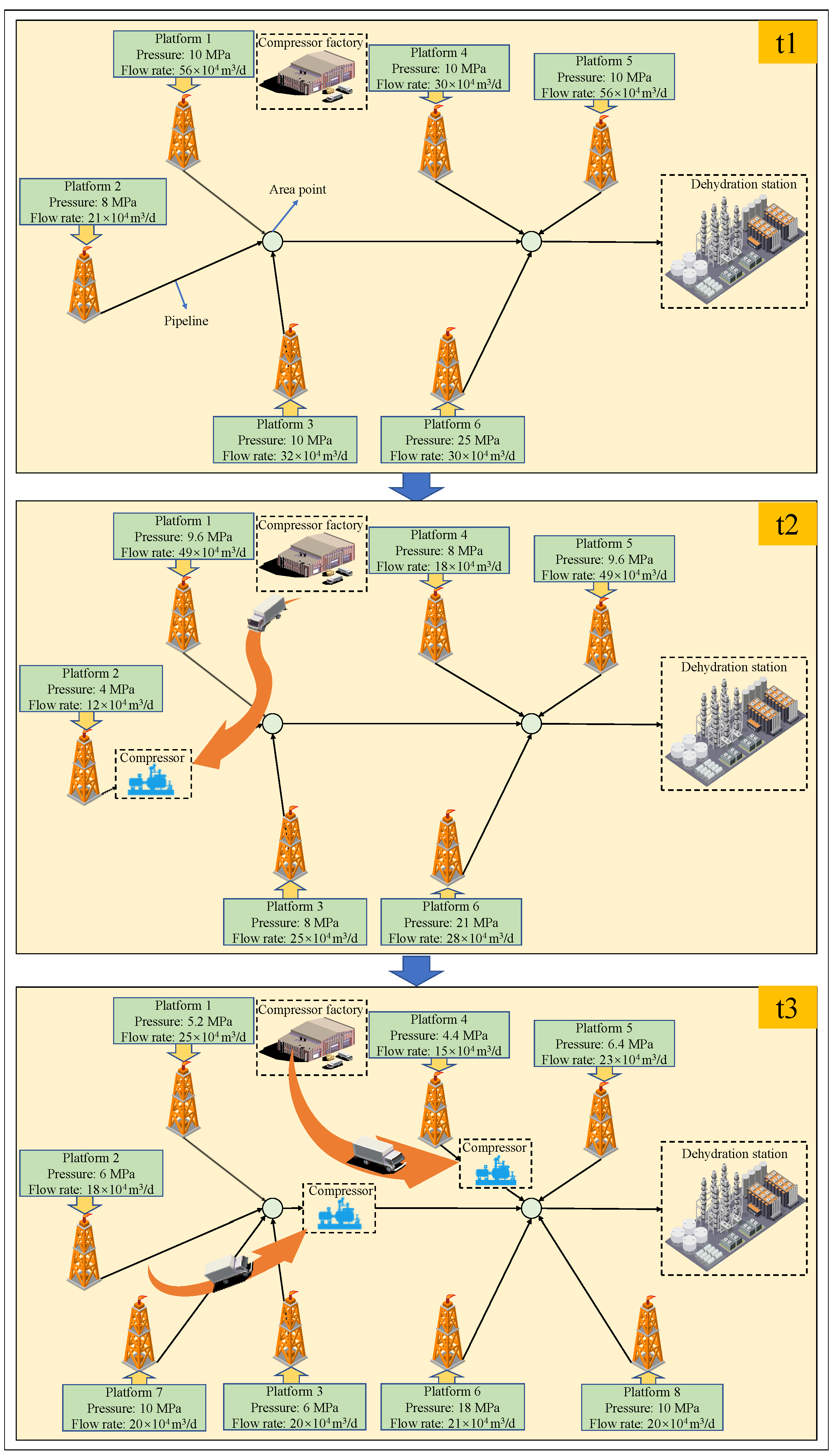
2. Problem Description
- Platform pressurization is to arrange the compressor at the platform, as shown in Figure 2a.
- Area pressurization is to arrange the compressor at the point of the region to pressurize the low-pressure area, as shown in Figure 2b.
- Station pressurization is to arrange the compressor at the station, as shown in Figure 2c.
- Well pressurization is to arrange the compressor to pressurize the single well or the same half-branch well inside the platform, as shown in Figure 2d.
- The shale gas production time can be divided into a series of short, discrete periods (Allen et al., 2018) [19].
- The shale gas production parameters do not change within a unit time period.
- During the specified shale gas production period, the modular compressors will not be damaged or require additional maintenance costs.
- The lead time for purchasing modular compressors is not taken into consideration.
3. Mathematical Formulation
3.1. Objective Function
3.2. Constraint
3.2.1. Pipeline Pressure and Flowrate Constraints
3.2.2. Compressor Constraints
3.2.3. Well or Platform Throttling Constraints
3.2.4. Pressure Balance Constraints
3.2.5. Well Flow Rate Constraints
3.2.6. Compressor Rearrangement Constraints
4. Solution Approach
5. Case Study
5.1. Basic Parameters
5.2. Result Analysis
5.2.1. Iterative Solution
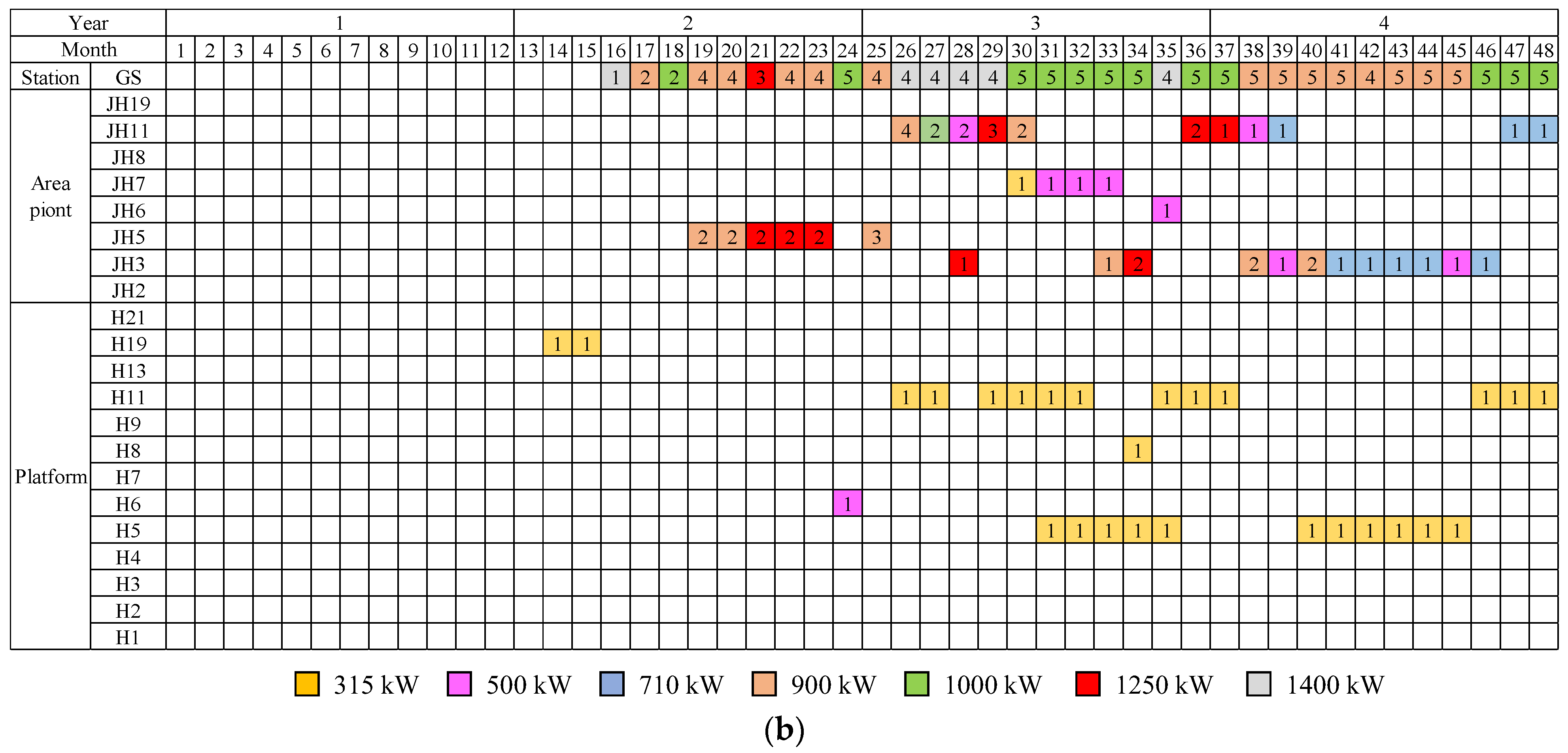
5.2.2. Type and Quantity of Modular Compressors
5.2.3. Pressurization Scheme
5.2.4. Operating Power
5.2.5. Economic Comparisons
6. Conclusions
- Concentrating on the changing characteristics of the pressurization process of shale gas production and considering the compressor modularization, this study established an MINLP model for the pressurization and rearrangement optimization of the SGGTS. The reliability of the model was verified by studying a practical example.
- By deploying the modular compressor, the idleness and waste of the modular compressor are avoided, the utilization rate of the modular compressor is greatly improved, and the production investment cost is also reduced to a certain extent, improving the economic benefits of the shale gas field.
- Under a multi-period condition, it requires fewer compressors and types, and the change in pressurizing position and rearrangement frequency of modular compressors are more stable, as is the change in compressor operating power. In addition, the investment cost of shale gas field production can be reduced. After solving under multi-period conditions, the cumulative cost is reduced by 17.19%.
- Compared with the previous work, our model has made great progress. In future work, we will consider the related uncertainty factors to establish an optimization model for the pressurization and rearrangement of the SGGTS to produce a pressurization scheme with more application values.
Author Contributions
Funding
Data Availability Statement
Conflicts of Interest
Nomenclature
| Location variable, 0 or 1 | |
| Decision difference between the compressor location at time t and time t − 1 | |
| Nozzle hole diameter, mm | |
| Pipeline diameter, cm | |
| Operating power, kW | |
| Total cost, 104 Yuan | |
| Purchase cost, 104 Yuan | |
| Operation cost, 104 Yuan | |
| Rearrangement cost, 104 Yuan | |
| Gas-specific heat ratio | |
| Pipeline length, km | |
| Maximum operating power, kW/set | |
| Installation compressor number | |
| Rearrangement compressor number | |
| Maximum operation pressure, MPa | |
| Minimum operation pressure of the pipeline, MPa | |
| Pressure in front of the nozzle, MPa | |
| Pressure behind the nozzle, MPa | |
| Node i pressure, MPa | |
| Well w pressure, MPa | |
| Platform g pressure, MPa | |
| Area point n pressure, MPa | |
| Station s pressure, MPa | |
| Suction pressure, MPa | |
| Discharge pressure, MPa | |
| Pipeline starting pressure, MPa | |
| Pipeline end pressure, MPa | |
| Smallest well pressure, MPa | |
| Node i flow rate, m3/min | |
| Well w initial flow rate, m3/d | |
| Well w flow rate, m3/d | |
| Flow rate through the nozzle in standard condition, m3/d | |
| Node i flow rate of the pipeline (i, j), m3/d | |
| Maximum flow rate through the nozzle, m3/d | |
| Pipeline flow rate, m3/d | |
| Operating price, 104 Yuan/kW | |
| Temperature in front of the nozzle, K | |
| Temperature in the pipeline (i, j), K | |
| Type y compressor number rearranged, set | |
| Type y compressor number installed, set | |
| Compressibility factor | |
| Compressibility factor under temperature T1 and pressure p1 | |
| Compressibility factor under the inlet condition | |
| Compressibility factor under the outlet condition | |
| Conversion factor | |
| Compression efficiency | |
| Relative density | |
| Gas adiabatic index, take for calculation example 1 | |
| Compressor price of type y, 104 Yuan/set | |
| Rearrangement price, 104 Yuan/set | |
| Compression ratio | |
| Well w throttle ratio | |
| Platform g throttle ratio | |
| Set of wells at platform g | |
| Number of 1 defined in the set | |
| Number of −1 defined in the set | |
| Difference value |
References
- Zhou, J.; Zhou, L.; Liang, G.; Wang, S.; Fu, T.; Zhou, X.; Peng, J. Optimal design of the gas storage surface pipeline system with injection and withdrawal conditions. Petroleum 2021, 7, 102–116. [Google Scholar] [CrossRef]
- Wei, J.; Duan, H.; Yan, Q. Shale gas: Will it become a new type of clean energy in China?—A perspective of development potential. J. Clean. Prod. 2021, 294, 126257. [Google Scholar] [CrossRef]
- Vengosh, A.; Warner, N.; Jackson, R.; Darrah, T. The Effects of Shale Gas Exploration and Hydraulic Fracturing on the Quality of Water Resources in the United States. Procedia Earth Planet. Sci. 2013, 7, 863–866. [Google Scholar] [CrossRef]
- Yuan, J.L.; Deng, J.G.; Tan, Q.; Yu, B.H.; Jin, X.C. Borehole stability analysis of horizontal drilling in shale gas reservoirs. Rock Mech. Rock Eng. 2013, 46, 1157–1164. [Google Scholar] [CrossRef]
- Lin, Y.; Liu, S.; Gao, S.; Yuan, Y.; Wang, J.; Xia, S. Study on the optimal design of volume fracturing for shale gas based on evaluating the fracturing effect-A case study on the Zhao Tong shale gas demonstration zone in Sichuan, China. J. Pet. Explor. Prod. 2021, 11, 1705–1714. [Google Scholar] [CrossRef]
- Real-Miranda, R.; López-Barrientos, J.D. A Geologic-Actuarial Approach for Insuring the Extraction Tasks of Non-Renewable Resources by One and Two Agents. Mathematics 2022, 10, 2022. [Google Scholar] [CrossRef]
- Cafaro, D.C.; Drouven, M.G.; Grossmann, I.E. Continuous-time formulations for the optimal planning of multiple refracture treatments in a shale gas well. AIChE J. 2018, 64, 1511–1516. [Google Scholar] [CrossRef]
- Drouven, M.G.; Grossmann, I.E.; Cafaro, D.C. Stochastic programming models for optimal shale well development and refracturing planning under uncertainty. AIChE J. 2017, 63, 4799–4813. [Google Scholar] [CrossRef]
- Grossmann, I.E.; Cafaro, D.C.; Yang, L. Optimization models for optimal investment, drilling, and water management in shale gas supply chains. Comput. Aided Chem. Eng. 2014, 34, 124–133. [Google Scholar]
- Tavallali, M.S.; Karimi, I.A.; Teo, K.M.; Baxendale, D.; Ayatollahi, S. Optimal producer well placement and production planning in an oil reservoir. Comput. Chem. Eng. 2013, 55, 109–125. [Google Scholar] [CrossRef]
- Cafaro, D.C.; Grossmann, I.E. Strategic planning, design, and development of the shale gas supply chain network. AIChE J. 2014, 60, 2122–2142. [Google Scholar] [CrossRef]
- Yang, L.; Grossmann, I.E.; Mauter, M.S.; Dilmore, R.M. Investment optimization model for freshwater acquisition and wastewater handling in shale gas production. AIChE J. 2015, 61, 1770–1782. [Google Scholar] [CrossRef]
- Drouven, M.G.; Grossmann, I.E. Multi-period planning, design, and strategic models for long-term, quality-sensitive shale gas development. AIChE J. 2016, 62, 2296–2323. [Google Scholar] [CrossRef]
- Cafaro, D.C.; Drouven, M.G.; Grossmann, I.E. Optimization models for planning shale gas well refracture treatments. AIChE J. 2016, 62, 4297–4307. [Google Scholar] [CrossRef]
- Mahmoud, M.; Aleid, A.; Ali, A.; Kamal, M.S. An integrated work flow to perform reservoir and completion parametric study on a shale gas reservoir. J. Pet. Explor. Prod. Technol. 2020, 10, 1497–1510. [Google Scholar] [CrossRef]
- Peng, Z.; Li, C.; Grossmann, I.E.; Kwon, K.; Ko, S.; Shin, J.; Feng, Y. Multi-period design and planning model of shale gas field development. AIChE J. 2021, 67, e17195. [Google Scholar] [CrossRef]
- Gao, J.; You, F. Can modular manufacturing be the next game-changer in shale gas supply chain design and operations for economic and environmental sustainability? ACS Sustain. Chem. Eng. 2017, 5, 10046–10071. [Google Scholar] [CrossRef]
- Yang, M.; You, F. Modular methanol manufacturing from shale gas: Techno-economic and environmental analyses of conventional large-scale production versus small-scale distributed, modular processing. AIChE J. 2018, 64, 495–510. [Google Scholar] [CrossRef]
- Allen, R.C.; Allaire, D.; El-Halwagi, M.M. Capacity planning for modular and transportable infrastructure for shale gas production and processing. Ind. Eng. Chem. Res. 2018, 58, 5887–5897. [Google Scholar] [CrossRef]
- Hong, B.; Li, X.; Song, S.; Chen, S.; Zhao, C.; Gong, J. Optimal planning and modular infrastructure dynamic allocation for shale gas production. Appl. Energy 2020, 261, 114439. [Google Scholar] [CrossRef]
- Hong, B.; Li, X.; Cui, X.; Gao, J.; Li, Y.; Gong, J.; Liu, H. General optimization model of modular equipment selection and serialization for shale gas field. Front. Energy Res. 2021, 9, 341. [Google Scholar] [CrossRef]
- Baldea, M.; Edgar, T.F.; Stanley, B.L.; Kiss, A.A. Modular manufacturing processes: Status, challenges, and opportunities. AIChE J. 2017, 63, 4262–4272. [Google Scholar] [CrossRef]
- Pakizer, K.; Fischer, M.; Lieberherr, E. Policy instrument mixes for operating modular technology within hybrid water systems. Environ. Sci. Policy 2020, 105, 120–133. [Google Scholar] [CrossRef]
- Lier, S.; Grünewald, M. Net present value analysis of modular chemical production plants. Chem. Eng. Technol. 2011, 34, 809–816. [Google Scholar] [CrossRef]
- Palys, M.J.; Allman, A.; Daoutidis, P. Exploring the benefits of modular renewable-powered ammonia production: A supply chain optimization study. Ind. Eng. Chem. Res. 2018, 58, 5898–5908. [Google Scholar] [CrossRef]
- Tan, S.H.; Barton, P.I. Optimal dynamic allocation of mobile plants to monetize associated or stranded natural gas, part I: Bakken shale play case study. Energy 2015, 93, 1581–1594. [Google Scholar] [CrossRef]
- Tan, S.H.; Barton, P.I. Optimal dynamic allocation of mobile plants to monetize associated or stranded natural gas, part II: Dealing with uncertainty. Energy 2016, 96, 461–467. [Google Scholar] [CrossRef]
- Zhou, J.; Peng, J.; Liang, G.; Deng, T. Layout optimization of Tree-Tree gas pipeline Network. J. Pet. Sci. Eng. 2019, 173, 666–680. [Google Scholar] [CrossRef]
- Belotti, P. Couenne: A User’s Manual; Technical Report; Lehigh University: Bethlehem, PA, USA, 2009. [Google Scholar]
- Duran, M.A.; Grossmann, I.E. An outer-approximation algorithm for a class of mixed-integer nonlinear programs. Math. Program. 1987, 39, 337. [Google Scholar] [CrossRef]
- Drud, A. CONOPT: A GRG code for large sparse dynamic nonlinear optimization problems. Math. Program. 1985, 31, 153–191. [Google Scholar] [CrossRef]
- Kronqvist, J.; Bernal, D.E.; Lundell, A.; Grossmann, I.E. A review and comparison of solvers for convex MINLP. Optim. Eng. 2018, 2, 397–455. [Google Scholar] [CrossRef]


| Number | Platform | Well Number | Production Time | Number | Platform | Well Number | Production Time |
|---|---|---|---|---|---|---|---|
| 1 | H1 | 8 | M1 | 8 | H8 | 3 | M19 |
| 2 | H2 | 4 | M1 | 9 | H9 | 6 | M19 |
| 3 | H3 | 3 | M15 | 10 | H11 | 3 | M10 |
| 4 | H4 | 3 | M16 | 11 | H19 | 3 | M16 |
| 5 | H5 | 4 | M21 | 12 | H21 | 3 | M1 |
| 6 | H6 | 8 | M1 | 13 | H13 | 4 | M1 |
| 7 | H7 | 1 | M24 | - | - | - | - |
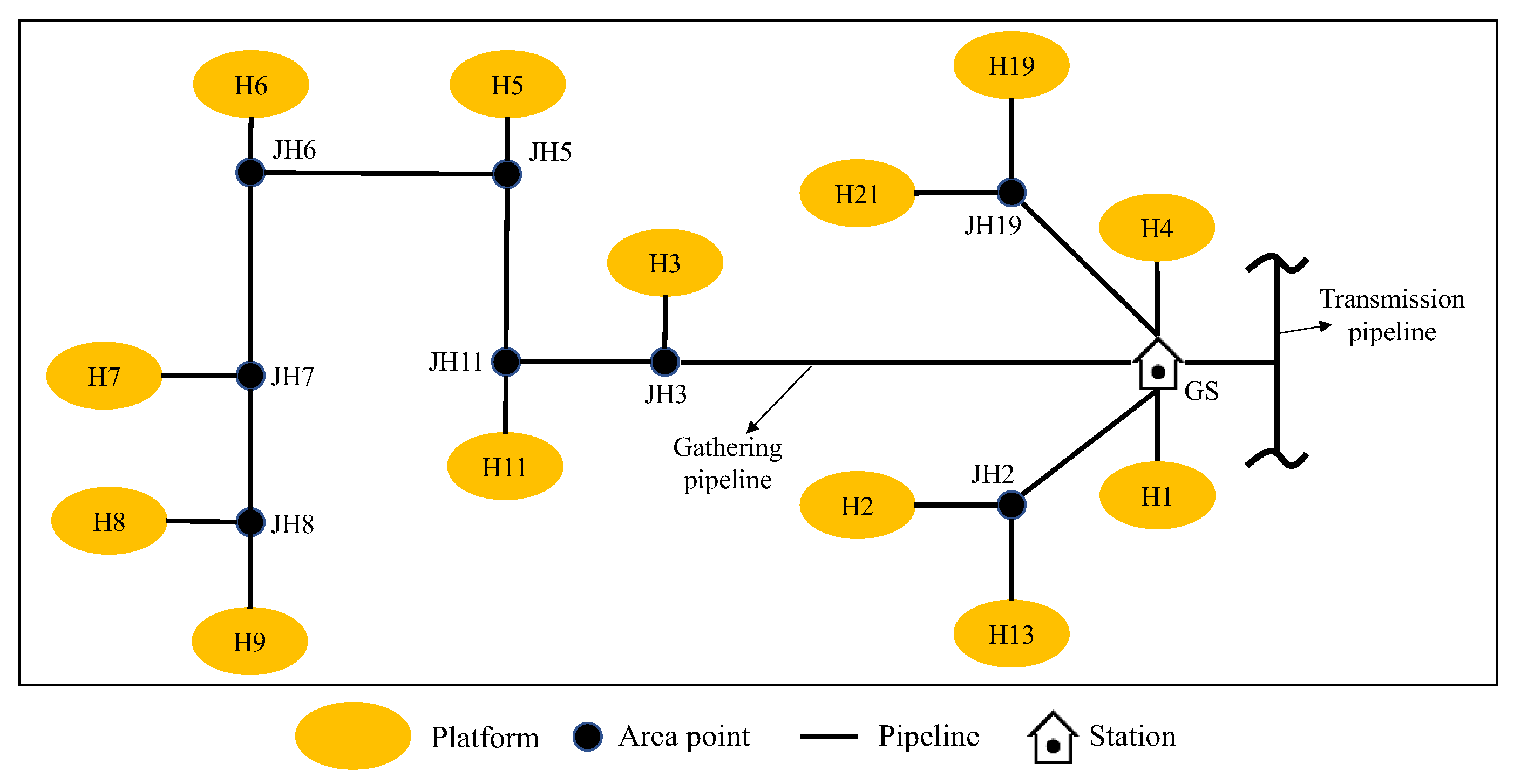
| Pipeline | Starting | End | Diameter (mm) | Length (km) |
|---|---|---|---|---|
| 1 | H1 | GS | 200 | 0.2 |
| 2 | H2 | GS | 200 | 1.4 |
| 3 | H3 | GS | 200 | 1.5 |
| 4 | H4 | GS | 200 | 4.4 |
| 5 | H5 | H11 | 200 | 2.7 |
| 6 | H6 | H5 | 200 | 3.2 |
| 7 | H7 | H6 | 200 | 2.8 |
| 8 | H8 | H7 | 200 | 2.1 |
| 9 | H9 | H8 | 200 | 1.3 |
| 10 | H11 | H3 | 200 | 2.6 |
| 11 | H13 | H2 | 200 | 6.2 |
| 12 | H19 | GS | 200 | 8.2 |
| 13 | H21 | H19 | 200 | 5.5 |
| Composition | CH4 | C2H6 | C3+ | CO2 | H2S | He | H2 | N2 |
|---|---|---|---|---|---|---|---|---|
| Mol (%) | 99.09 | 0.44 | 0.02 | 0.27 | 0.00 | 0.02 | 0.00 | 0.16 |
| Number | Compressor Power | Purchase Price (104 Yuan/Set) | Rearrangement Price (104 Yuan/Set) |
|---|---|---|---|
| 1 | 315 kW | 63 | 5 |
| 2 | 500 kW | 96 | 5 |
| 3 | 710 kW | 136 | 5 |
| 4 | 900 kW | 170 | 5 |
| 5 | 1000 kW | 190 | 5 |
| 6 | 1250 kW | 240 | 5 |
| 7 | 1400 kW | 270 | 5 |
| Time Period (Month) | CPU Time (s) | Iteration Count | Time Period (Month) | CPU Time (s) | Iteration Count |
|---|---|---|---|---|---|
| 14 | 0.20 | 696 | 32 | 0.15 | 1140 |
| 15 | 0.10 | 737 | 33 | 0.17 | 1050 |
| 16 | 0.09 | 900 | 34 | 0.60 | 1164 |
| 17 | 0.09 | 944 | 35 | 0.20 | 1062 |
| 18 | 0.11 | 1021 | 36 | 0.66 | 864 |
| 19 | 0.48 | 819 | 37 | 0.53 | 1179 |
| 20 | 0.38 | 1091 | 38 | 0.75 | 1239 |
| 21 | 0.44 | 864 | 39 | 0.58 | 1304 |
| 22 | 0.72 | 1100 | 40 | 0.17 | 1451 |
| 23 | 0.41 | 1044 | 41 | 0.11 | 1317 |
| 24 | 0.52 | 1118 | 42 | 0.15 | 715 |
| 25 | 0.22 | 1039 | 43 | 0.14 | 1197 |
| 26 | 0.11 | 1236 | 44 | 0.18 | 1227 |
| 27 | 0.13 | 1107 | 45 | 0.18 | 1274 |
| 28 | 0.32 | 1189 | 46 | 0.17 | 1285 |
| 29 | 0.48 | 763 | 47 | 0.11 | 1147 |
| 30 | 0.14 | 1496 | 48 | 0.16 | 1051 |
| 31 | 0.18 | 1076 | - | - | - |
Disclaimer/Publisher’s Note: The statements, opinions and data contained in all publications are solely those of the individual author(s) and contributor(s) and not of MDPI and/or the editor(s). MDPI and/or the editor(s) disclaim responsibility for any injury to people or property resulting from any ideas, methods, instructions or products referred to in the content. |
© 2023 by the authors. Licensee MDPI, Basel, Switzerland. This article is an open access article distributed under the terms and conditions of the Creative Commons Attribution (CC BY) license (https://creativecommons.org/licenses/by/4.0/).
Share and Cite
Wu, K.; Yang, J.; Lin, Y.; Zhou, P.; Luo, Y.; Wang, F.; Liu, S.; Zhou, J. A Multi-Period Model of Compressor Scheme Optimization for the Shale Gas Gathering and Transportation System. Processes 2023, 11, 3101. https://doi.org/10.3390/pr11113101
Wu K, Yang J, Lin Y, Zhou P, Luo Y, Wang F, Liu S, Zhou J. A Multi-Period Model of Compressor Scheme Optimization for the Shale Gas Gathering and Transportation System. Processes. 2023; 11(11):3101. https://doi.org/10.3390/pr11113101
Chicago/Turabian StyleWu, Kunyi, Jianying Yang, Yu Lin, Pan Zhou, Yanli Luo, Feng Wang, Shitao Liu, and Jun Zhou. 2023. "A Multi-Period Model of Compressor Scheme Optimization for the Shale Gas Gathering and Transportation System" Processes 11, no. 11: 3101. https://doi.org/10.3390/pr11113101