
Online Dynamic Optimization of Multi-Rate Processes with the Case of a Fluid Catalytic Cracking Unit

Department of Automation, China University of Petroleum, Beijing 102249, China
*
Author to whom correspondence should be addressed.
Processes 2023, 11(11), 3088; https://doi.org/10.3390/pr11113088
Submission received: 3 October 2023
/
Revised: 21 October 2023
/
Accepted: 24 October 2023
/
Published: 27 October 2023
(This article belongs to the Special Issue Chemical Process Modelling and Simulation)
Abstract
:Due to operational limitations in the industrial field, the operating variables of fluid catalytic cracking units (FCCU) are of multiple operating frequencies, which are CO combustion promoter amount, recycle slurry flow rate, combustion air flow rate, heat escape, and reaction temperature, from low frequency to high frequency. There are usually two schemes for operation optimization of FCCU. The former is called single-rate, single-window optimization, whose operating variables are optimized only once in the whole operation cycle, which is easy to achieve, but the optimization effect is poor. The latter is called single-rate multi-window optimization, whose operating variables are optimized repeatedly and whose operation cycle is discretized into multiple optimization periods with the same frequency, which costs a heavy calculation burden and cannot adapt to the optimization variables with multiple operating frequencies. So, a multi-rate, variable-window online dynamic optimization method is proposed. In an operation cycle, the high-frequency operating variable is optimized in a short optimization period, and the low-frequency operating variable is optimized in a long optimization period; each optimization period has integer multiples to the minimum optimization period. Each optimized result for each optimization period is put into use online immediately. The optimization model involves the time domain differential equations, integral cost objective function, and measured disturbances. The experimental results show that compared with the single-rate, single-window optimization method and single-rate multi-window optimization method, the optimization effect of multi-rate, variable-window online dynamic optimization is better than single-rate, single-window optimization but worse than single-rate multi-window optimization. However, the optimization results are consistent with the operation frequency of each optimization variable, which can be implemented in complex chemical processes and increase certain economic benefits.
1. Introduction
A system with two or more operating frequencies is usually called a multi-rate system [1,2,3]. In chemical processes, there commonly exist multi-rate systems [4,5,6]. It is passively generated due to the process constraints of production, safety, economy, or environment, and on the other hand, it is artificially constructed due to the need for process control [7,8,9]. The multi-rate problem mainly exists for the following reasons: (1) the implementation of dynamic optimization is limited by operation rate [10,11,12]; (2) in the actual process, the number of sensors is less than the number of output variables, so time-sharing measurement is adopted [13,14,15]; (3) in the chemical process, the change frequency for each optimization variable may greatly differ from others; (4) in addition to the multi-rate phenomenon in the actual process, some operation optimizations require multi-rate operation [16,17,18], such as pole assignment, enhanced dynamic performance, and model following [19,20,21]. The multi-rate problem exists widely in petrochemical, metallurgical, and power industries, and it has an increasingly important impact on the monitoring and diagnosis of production processes [22,23,24]. Therefore, deep research on multi-rate dynamic optimization is inevitable for the development of industrial production.
In the 1950s, scholars began to study the online dynamic optimization problems of the multi-rate process [25,26]. With the acceleration of the industrial process, the application of large equipment and complex devices has become more extensive. For the study of complex systems, the optimization of multiple variables has also become more meaningful [27,28,29]. Therefore, the multi-rate optimization problem has attracted more and more researchers’ attention. In the current research, more researchers focus on multi-objective optimization, while the research on multi-objective online dynamic optimization is relatively less [30,31,32]. Due to computer performance limitations, classical methods were mainly used for optimization during the early period of research on the topic. Kranc was the first scholar to study multi-rate, variable-window online dynamic optimization, and the Kranc operator method is still an effective method for analyzing multi-rate systems [33,34,35]. Araki and Yamamoto provided a complete state space model of multi-rate, variable-window online dynamic optimization. Subsequently, on the basis of lifting technology, the theory of multi-rate systems has gradually developed, which has been integrated with multiple disciplines, such as controllability and observability, system identification, soft measurement, signal processing, data fusion, etc. [36,37,38]. At the same time, the online dynamic optimization research of multi-rate, variable-window systems continuously absorbs excellent ideas from other research fields, which provides a better optimization theoretical basis for the cross-integration of multi-rate systems and other fields [39].
This paper mainly focuses on the multi-rate, variable-window online dynamic optimization of heavy oil fluid catalytic cracking unit (FCCU). FCCU is an important part of oil refinery [40,41]. FCCU involves multiple operating variables with multiple operating frequencies, so it is a typical multi-rate system. The carbon residue value of FCCU feedstock oil is low, and light oil yield can be improved by adjusting the CO combustion promoters and combustion air flow rate [42,43]. When the feedstock oil is heavy oil, it is necessary to combine the adjustment methods of heat escape and recycling the slurry. Adjusting the amount of recycled slurry can effectively reduce coke yield [44,45]. Heat escape removes excess heat through the external catalyst cooler to control the regenerator temperature. This paper mainly discusses how to effectively improve the economic benefits when FCCU feedstock is heavy oil. When the feedstock is heavy oil, five optimization variables are selected for online dynamic optimization of the multi-rate process [46,47]. The five optimization variables are CO combustion promoters, combustion air flow rate, heat escape, recycle slurry flow rate, and reaction temperature. Simulation experiments show that the light oil yield can be effectively improved by multi-rate, variable-window online dynamic optimization.
The rest of this paper is organized as follows: in Section 2, the expansion of the heavy oil catalytic cracking model and multi-rate, variable-window online dynamic optimization analysis are mainly described. In Section 3, the problem is described, and a multi-rate, variable-window online dynamic optimization method is proposed. Then, single-rate, single-window full-cycle one-time optimization and single-rate multi-window full-cycle one-time optimization are studied in detail, and the advantages and disadvantages of the two optimization methods are summarized. The above methods are applied to the catalytic cracking unit for simulation. Based on the above research, in order to improve the practicability of the optimization method, the multi-rate, variable-window online dynamic optimization method can be used. In Section 4, the multi-rate, variable-window online dynamic optimization process is provided in detail, and the solution is studied. In Section 5, the operating conditions and operating characteristics of the catalytic cracking unit under standard conditions are studied, and an example of FCCU is presented. Through experimental comparison, it is found that the multi-rate, variable-window online dynamic optimization method is not only suitable for complex chemical processes but can also effectively improve economic benefits. Finally, the dynamic performance of multi-rate, variable-window online dynamic optimization is studied.
2. Expansion of Heavy Oil FCCU Model and Multi-Rate, Variable-Window Online Dynamic Optimization Analysis
Due to the shortage of petroleum resources, the heavierization of feedstock oil is a trend. When feedstock oil is heavy oil, the production requirements cannot be met only by adjusting the CO combustion promoters and the combustion air flow rate. Therefore, the model is expanded to improve the light oil yield combined with other adjustment methods. The model in this paper is based on FCCU with a high-efficiency regenerator of pre-combustor, and the extended part is an external catalyst cooler. A schematic diagram of the model is shown in Figure 1 [48].
In this study, the reaction kinetics model adopts a five-lump model, which is expressed as follows.
All cracking reactions and catalyst deactivation reactions are treated as first-order reactions. The FCCU process contains multiple frequency operation modes, which is a typical multi-rate, variable-window system. Here, we selected five representative variables as the research object: (reaction temperature, Triser), (heat escape, Qs), (combustion air flow rate, Vrg1), (recycle slurry flow rate, Fslurry), and (CO combustion promoters, Mpro).
In order to verify the feasibility of multi-rate, variable-window online dynamic optimization in FCCU, the method of experimental comparative analysis was used. In the process of experiment, there were three groups of comparative experiments, and the whole optimization period was 8 h. Experiment 1 shows that the optimization period of variables , , , , and are all 8 h; that is, the process is single-rate, single-window full cycle one-time optimization. Experiment 2: The optimization period of variables , , , , and are all 15 min; that is, the process is a single-rate multi-window full cycle one-time optimization. Experiment 3: The optimization periods of variables , , , , and are 15 min, 1 h, 2 h, 4 h, and 8 h, respectively. This process is a multi-rate, variable-window online dynamic optimization. During multi-rate, variable-window online dynamic optimization, the system starts at time 0, and the five variables run in turn according to the initial state. Because the operation period of reaction temperature is the shortest, the refresh frequency is the fastest. Under the action of the starting factor, the dynamic optimization rate of temperature is relatively fast. When the time reaches 1 h, the external catalyst cooler starts to be dynamically optimized. As time goes on, the other three variables are optimized in turn.
3. Necessity Analysis and Mathematical Description of Multi-Rate, Variable-Window Online Dynamic Optimization
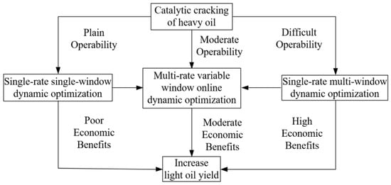
3.1. Single-Rate Optimization and Multi-Rate Optimization
Generally, all operation variables are optimized only once in the whole operation cycle, or the operation cycle can be discretized at the same frequency, and all operation variables are optimized in the corresponding discretization optimization period. The former can be called single-rate, single-window control vector parameterization (CVP) of full-cycle one-time optimization, and the latter can be called single-rate multi-window CVP of full-cycle one-time optimization. When the system is steady, the optimization period will be long. Generally, single-rate, single-window CVP can be used. Single-rate, single-window CVP is easy to use, and the optimization effect is not ideal. For single-rate multi-window CVP, a large amount of calculation must be carried out in the optimization process, but compared with the poor operability, the optimization effect will be better. However, the common shortcoming of both is poor practicality. The main reason is that the operation variables must have multiple operation frequencies due to the operation limitation of the industrial field. Therefore, a new dynamic optimization method is proposed, namely the multi-rate, variable-window online dynamic optimization method. This method can not only trade off the advantages of the two single-rate CVPs but also effectively improve practicability.
The multi-rate, variable-window online dynamic optimization discretizes multiple optimization variables according to the actual operating frequency of each optimization variable, and it transforms the dynamic optimization problem into a nonlinear programming problem with differential algebraic equation constraints. The most common parameterization method is the time segment strategy; that is, every optimization variable is approximated as a constant in each segment, and each time segment is the same as the actual operation period of the optimization variable. By discretizing the optimization variables, the optimization results can be infinitely approached to the optimal trajectory.
In order to illustrate the characteristics of multi-rate, variable-window online dynamic optimization, we first analyzed the single-rate, single-window optimization and single-rate multi-window optimization and then compared them with multi-rate, variable-window online dynamic optimization.
3.2. Mathematical Description of Single-Rate, Single-Window Optimization
In the process industry, it is not easy for production to reach the ideal state, so operation optimization is commonly used to operate the production process. Here, the single-rate, single-window CVP method was analyzed. The decision variables of dynamic optimization were , and the optimization period of all variables was Tm. The entire time domain of optimization was Tm; that is, there were m optimization variables in the system, and the refresh time of all variables was the entire optimization period. The optimization variables were optimized only once in the entire time domain, and the expression was as follows. After the above optimization process, the optimization window continued to move forward.
When the optimization time ∈ [0, Tm], the mathematical expression was:
Let ; then, is the general expression of the objective function, and the basic goal is to minimize the additional cost while maximizing product yield. In all the mathematical expressions, j represents a function, (, ) represents the vector of (differential, algebraic) state variables, u represents the optimization vector, φ represents other constraints of the system, and (, ) represents the set of (differential, algebraic) equations.
The single-rate, single-window CVP method was adopted, and the optimization variable was a constant value in the whole operation cycle. The single-rate, single-window CVP method is common in the field of process control, but it has obvious advantages and disadvantages.
Advantages: (1) The number of optimizations is relatively small. Because all optimization objectives are a single-rate, single-window, only one optimization is required for optimization variables. For process engineering, it is relatively easy to implement. (2) The optimization process is simple.
Disadvantages: The method has poor practicality. In the field of process control, the system is generally a relatively complex system. Although the optimization variables are not single, the optimization results are not ideal. Therefore, it has certain limitations for the single-rate, single-window CVP method.
3.3. Mathematical Description of Single-Rate Multi-Window Optimization
Due to the unsatisfactory effect of the single-rate, single-window CVP method, the single-rate multi-window CVP method was studied. The analysis of the single-rate multi-window CVP method is shown in Figure 2.
In Figure 2, the time corresponding to each black grid and gray grid is equal to T. Among them, the black grid and gray grid represent the same optimization window. When the system is optimized, all optimization variables are optimized by one-time, single-rate, multi-window, full-cycle optimization. The update period of the optimization variables of dynamic optimization are all T, and Tm = qT; then, are optimized at the same time every T time. Then, all the optimization variables are optimized q times in the whole cycle, and the expression of optimization variables is as follows. In the process of system optimization, after completing an optimization cycle, the optimization window will continue to move forward and start a new optimization process.
When the optimization time ∈ [0, Tm], the mathematical expression is.
For the single-rate, multi-window CVP method, the optimization variables are continuously optimized in the whole cycle so that the optimization variables are closer to the optimal value. The single-rate multi-window CVP method in some specific objects is of ideal optimization effect. However, there are some advantages and disadvantages of the single-rate, multi-window CVP method.
Advantages: the optimization effect is better because the single-rate, multi-window CVP method uses multiple optimizations for all optimization variables. The more optimization times in the full cycle, the better the results will be.
Disadvantages: (1) It takes a long time to complete the optimization. The single-rate, multi-window CVP method is a relatively more refined optimization method. Compared with the single-rate, single-window CVP method, the faster optimization operation frequency of the single-rate, multi-window CVP method is required, which not only poses certain challenges to the dynamic performance of the program but also makes the program more redundant. (2) Poor practicality. In the field of control, if the single-rate, multi-window CVP method is used for optimization, the applicable scope will be reduced. Therefore, it is difficult to realize.
3.4. Multi-Rate, Variable-Window Online Dynamic Optimization Research and Process Description
In the production process, the system is generally in a state of dynamic balance, so it is more in line with the needs of production to study multi-rate, variable-window online dynamic optimization. In online dynamic optimization of multi-rate, variable-window systems, reasonable optimization variables should be selected. Here, we conducted a detailed study of the online dynamic optimization process of a multi-rate, variable-window system, as shown in Figure 3.
In Figure 3 above, u0 is the input variable, and d is the measured disturbance. The conventional optimization method is that under the action of input variable u0 and disturbance d, the system output result is y. When multi-rate, variable-window online dynamic optimization is carried out, the output result of the system is under the action of input variable u0 and disturbance d. Through the online adjustment of dynamic optimization, the output of the system is better. In multi-rate, variable-window online dynamic optimization, J1 is solved first. In this process, u1 performs dynamic optimization, while u2, u3, …, um remain unchanged. When solving J2, u1 and u2 are dynamically optimized, while u3, …, um remain unchanged. According to the above optimization process, when solving Jm, u1, u2, …, um are dynamically optimized.
The online dynamic optimization process of a multi-rate, variable-window system is studied, as shown in Figure 4. m variables are selected as optimization variables. Then, the optimization periods of optimization variables , , …, are, respectively, , , …, . Assuming that the optimization result is obtained by the i-th component ui of i = 1, 2, …, m after the action of the optimization period Ti, the following relationship is satisfied between the optimization components.
where qi is a positive integer, and T is the basic optimization period of the control system. Let q be the least common multiple of all qi; that is,
Here, let
Then, Tm is the cycle period of the whole system.
Through the above definition and analysis,
In the above formula, , () are set as positive integers, and T1 < T2 < … < Tm.
In the online dynamic optimization of a multi-rate, variable-window system, the optimization variable with the shortest period is first selected for dynamic optimization. As time goes on, the optimization variable with the second optimization period begins to be optimized. According to the above process, the remaining optimization variables are optimized in turn until the period Tm of the whole system ends. The online dynamic optimization process of the multi-rate, variable-window system is described as follows, and the change in optimization variables is shown in Table 1.
(1) When the optimization time ∈ [0, T2], the optimization variable of dynamic optimization is u1. U1 needs to be optimized q12 times, from to , while other variables remain unchanged. The vector expression of optimization variables is as follows.
The mathematical expression is:
(2) When the optimization time ∈ [T2, T3], u1 and u2 are optimized, and other variables remain unchanged. In this process, u1 is optimized q12 times, from to . U2 needs to be optimized once, from to . The vector expression of the optimization variables is as follows.
The mathematical expression is:
(3) When the optimization time ∈ [T3, Tm−1], u1, u2, and u3 are optimized, and other variables remain unchanged. In this process, u1 is optimized q13 times, from to . U2 needs to be optimized q23 times, from to . U3 needs to be optimized once, from to . The vector expression of the optimization variables is as follows.
The mathematical expression is:
(4) When the optimization time ∈ [Tm−1, Tm], variables are optimized. In this optimization process, u1 is optimized by q1(m−1) times and is optimized to . U2 needs to be optimized q2(m−1) times from to . U3 needs to be optimized q3(m−1) times from to . Other variables are optimized in turn according to the above process. Additionally, um−1 needs to be optimized once, from to . The vector expression of the optimization variables is as follows.
The mathematical expression is:
For constraint equations in the above mathematical expressions, including initial conditions, end-point constraints, and process constraints, 0 and Tm represent two end-point moments, and the initial conditions and end-point constraints are expressed as
The process constraints are expressed as
where (, ) and (, ) are the lower and upper bounds of (differential, algebraic) state variables; and are the lower and upper limits of the optimization variables; and are the lower and upper bound constraints on other conditions.
4. Multi-Rate, Variable-Window Online Dynamic Optimization Solution Process
For the online dynamic optimization solution of a multi-rate, variable-window system, the direct method is to solve the dynamic optimization problem as a nonlinear programming problem after time discretization. Both the full discretization method and the sequential method belong to the category of discrete methods. With the full discretization method, the optimization variables and differential variables will be discretized. The sequential method can use the operation means of control vector parameterization so that only the optimization variables are discretized. Compared with the full discretization method, the sequential method has obvious advantages. It can only act on the optimization variables in the process of discretization, which can effectively avoid the problem of high dimension problem caused by discretization.
If the full discretization method is used for online optimization, errors will be increased, and the accuracy requirement for discretization will be further increased. In addition, the dimension increase not only increases the optimization calculation cost but may also lead to the inability to obtain the optimal solution. Considering that the multi-rate, variable-window system usually has more differential variables than optimization variables, the multi-rate, variable-window method is used for online dynamic optimization. The values of state variables, objective functions, and constraint conditions can all be found by standard DAE solvers. The solution process of multi-rate, variable-window online dynamic optimization is shown in Figure 5. First, optimization is carried out through path I. Then, through path II, the solution is carried out according to the same process. Online dynamic optimization is carried out one by one until the end of the whole operation cycle.
For the online optimization process described in Figure 5, the optimization variables can be expressed as
In the formula, m represents the number of optimization variables and is also the dimension of the control vector. Here, we emphasize again that Tm is the dynamic optimization period of the whole system. In order to carry out the time grid division of the control time domain for all control vectors, we define the optimization period of ui as Ti. Due to different optimization periods, the number of update qi of ui in the whole optimization period must be different. Then, there is
Let , and .
Due to the different optimization periods of different control vectors, the control vectors can divide the time domain into the following forms.
The multi-rate, variable-window online dynamic optimization process can be understood as nested rolling optimization. In the above definition, it can be seen that the optimization frequency of u1 is the highest, then the optimization period of u1 is the smallest; similarly, the optimization period of um is the largest. Dynamic optimization starts from time 0, and all target vectors will go through a continuous optimization process. The online dynamic optimization solution process for multi-rate, variable-window systems is shown as follows.
Because the smallest nested optimization window is achieved when u1 and u2 are optimized at the same time, as time goes on, when time T2 < T, the optimization equation of u1 and u2 can be expressed as
When time T3 < T, the optimization equation of u3 can be expressed as
When time T4 < T, the optimization equation of u4 can be expressed as
According to the above online optimization process, the remaining optimization variables are optimized one by one. When the time is greater than Tm−1, um−1 performs dynamic optimization. The optimization equation is expressed as
When time Tm = T, the optimization equation of um can be expressed as follows
In the above online optimization process, each variable is in the state of rolling update over time. The shorter the optimization period is, the faster the update speed is. When the update time reaches Tm, dynamic optimization is completed. Then, the optimization window moves forward to start the next optimization cycle.
5. Experimental Study on Catalytic Cracking
5.1. Operating Characteristics of FCCU under Nominal Conditions
The operating characteristics of the reaction-regeneration system under nominal conditions after model expansion are shown in Table 2, while some important operating parameters as listed at Appendix A. In addition, our group conducted a detailed study on the activity characteristics of CO combustion promoters. In a single cycle, the average activity dynamic trend of mixed CO combustion promoters is the same as that of fresh CO combustion promoters, but the activity decrease is relatively gentle.
The operating characteristics of the heavy oil catalytic cracking system under nominal operating conditions are shown in Figure 6, while the detail model of the FCCU is given at Appendix B.
It can be seen from Figure 6a that, due to the gradual decreasing activity of CO combustion promoters, the coke-burning intensity gradually weakens, and the temperature of the spent catalysts is reduced. It can be found in Figure 6b that the carbon content of the spent catalysts gradually increases due to the weakening of coke burning. It can be seen from Figure 6c that the carbon content of feedstock oil is high, the coke-burning generates more heat, and the temperature of the dilute phase gradually increases with the reaction. It can be found from Figure 6d that due to the higher carbon content of spent catalysts, the O2 consumption in the coke-burning tank increases, leading to the gradual decrease of O2 content in flue gas. Figure 6e,f show that due to more heat generated in the coke-burning tank, the temperature of regenerated catalysts increases. Because the temperature needs to be controlled at the set point, the catalyst cycle flow rate decreases and the light oil yield decreases.
5.2. Case Analysis of Catalytic Cracking
The premise of the online dynamic optimization of FCCU is to ensure that the system is in a stable state and that reasonable optimization operation is carried out in the feasible region. The constraint conditions of decision variables and state variables are shown in Table 3 [35]. The dynamic optimization results for FCCU are shown in Figure 7.
Single-rate, single-window dynamic optimization is mathematically expressed as model 1:
Single-rate, multi-window dynamic optimization is mathematically expressed as model 2:
Multi-rate, variable-window online dynamic optimization is mathematically expressed as model 3:
where , , , , and respectively, represent gasoline benefit, diesel benefit, slurry
benefit, CO combustion promoters cost, and other energy consumption. , , , and are the prices of gasoline, diesel, slurry, and CO combustion promoters. rN, rD, g, and g′ represent gasoline production, diesel production, slurry production, and total recycled slurry. c1 represents the consumption of CO combustion promoters, and k1, k2, k3, and k4 are coefficients. In the formula , the first item is the energy consumption of the combustion air, the second item is the energy consumption of the recycled slurry, the third item is the heat getting outside energy consumption, and the fourth item is the heat energy of flue gas.
The detailed composition of the objective function values before and after the dynamic optimization of FCCU is shown in Table 4. It can also be seen from Table 4 that when there are disturbances, the economic benefits generated by multi-rate, variable-window online dynamic optimization are the highest. Under the condition of measured disturbance in the working process, the system continuously optimizes online so that the conversion rate of feedstock oil is improved, thus maximizing economic benefits. In the actual chemical process, the operation period of the above five variables will not be 8 h or 15 min at the same time. Because of poor practicability, it belongs to the case of taking extreme values. It is also to prove the superiority of multi-rate, variable-window online dynamic optimization. However, multi-rate, variable-window online dynamic optimization is more in line with the operation of chemical systems. Through experimental comparison, it is found that multi-rate, variable-window online dynamic optimization for complex chemical systems can effectively improve economic benefits.
In Figure 7, the solid line is the benchmark result before optimization. It can be seen from Figure 7a that the amount of CO combustion promoters is increased through single-rate, single-window dynamic optimization. This is because the optimization effect is poor, and the utilization rate of CO combustion promoters decreases, thus promoting the addition amount to increase. Single-rate, multi-window optimization and multi-rate variable-window, online dynamic optimization can effectively reduce the amount of CO combustion promoters. Figure 7b shows that under the action of dynamic optimization, the amount of recycled slurry increases. In multi-rate, variable-window dynamic optimization adjustment, recycle slurry is relatively high. As the optimization period is reduced, the utilization rate of the safety margin is increased, thus promoting the increase of recycled slurry. Because the effect of single-rate, single-window dynamic optimization is poor, in order to prevent overrunning temperature, the amount of recycled slurry increases less. From Figure 7c, it is found that combustion air not only promotes coke-burning but also acts as a coolant in the whole reaction process. Single-rate, single-window dynamic optimization adjustment reduces the safe operation interval of the system, and the increase of combustion air plays the role of the protection device. Single-rate, multi-window dynamic optimization adjustment increases the amount of recycled slurry. In order to promote coke-burning, the combustion air increases. Under the action of multi-rate, variable-window online dynamic optimization, it is beneficial to improve the working performance of the system and improve the utilization rate of the combustion air. It can be seen from Figure 7d that single-rate, single-window optimization can maximize heat escape. Because feedstock oil is heavy oil, more heat is produced in the process of coke-burning, and heat escape is increased to improve the stability of the system. For single-rate, multi-window optimization and multi-rate, variable-window dynamic optimization, heat escape is more prominent in the initial stage of the system, the activity of the CO combustion promoters is reduced, the degree of coke-burning is weakened, and heat escape is gradually reduced. Under the action of a temperature regulator, dynamic optimization makes the temperature gradually stable. As can be seen from Figure 7e, the reaction temperature is obviously increased by single-rate, single-window dynamic optimization. Due to the poor optimization effect and heat escape, the recycled slurry cannot adjust the temperature in time, resulting in an increase in the reaction temperature. Multi-rate, variable-window online dynamic optimization and single-rate, multi-window optimization have relatively good effects on temperature regulation. In addition, with the progress of the reaction, the activity of CO combustion promoters gradually decreases, coke-burning intensity decreases, and the reaction temperature gradually decreases.
The sensitivity analysis of light oil yield before and after dynamic optimization is shown in Figure 8 for heavy oil in FCCU by dynamic optimization adjustment. Figure 8a is the result of light oil yield before optimization. Figure 8b is the result of single-rate, single-window dynamic optimization. Figure 8c is the result of single-rate, multi-window dynamic optimization. Figure 8d is the result of multi-rate, variable-window online dynamic optimization. Compared with Figure 8a,b, it can be seen that because the dynamic optimization period is 8 h, , , , , and are constant values in a single period, and the optimization process is affected by the decrease of CO combustion promoters activity. The increase rate of gasoline is small, and the decrease rate of diesel is slow, so the decrease rate of light oil yield is slow. Comparing Figure 8a,c, it can be seen that the reduction of the optimization period can make the system working state closer to the optimal point and promote the improvement of light oil yield. With the increasing optimization time, the reduction of diesel yield decreases, the growth rate of gasoline increases, and the light oil yield increases. Finally, by comparing Figure 8a,d, it can be seen that with optimization, the gasoline yield increases rapidly, and the diesel yield decreases slightly. The increasing rate of gasoline is greater than the decreasing rate of diesel, so the light oil yield increases gradually. From the above experimental results, it can be seen that the multi-rate, variable-window online dynamic optimization adjustment is better than single-rate, single-window optimization and weaker than single-rate, multi-window optimization. Therefore, for complex chemical system processes, multi-rate, variable-window online dynamic optimization can improve economic benefits to a certain extent.
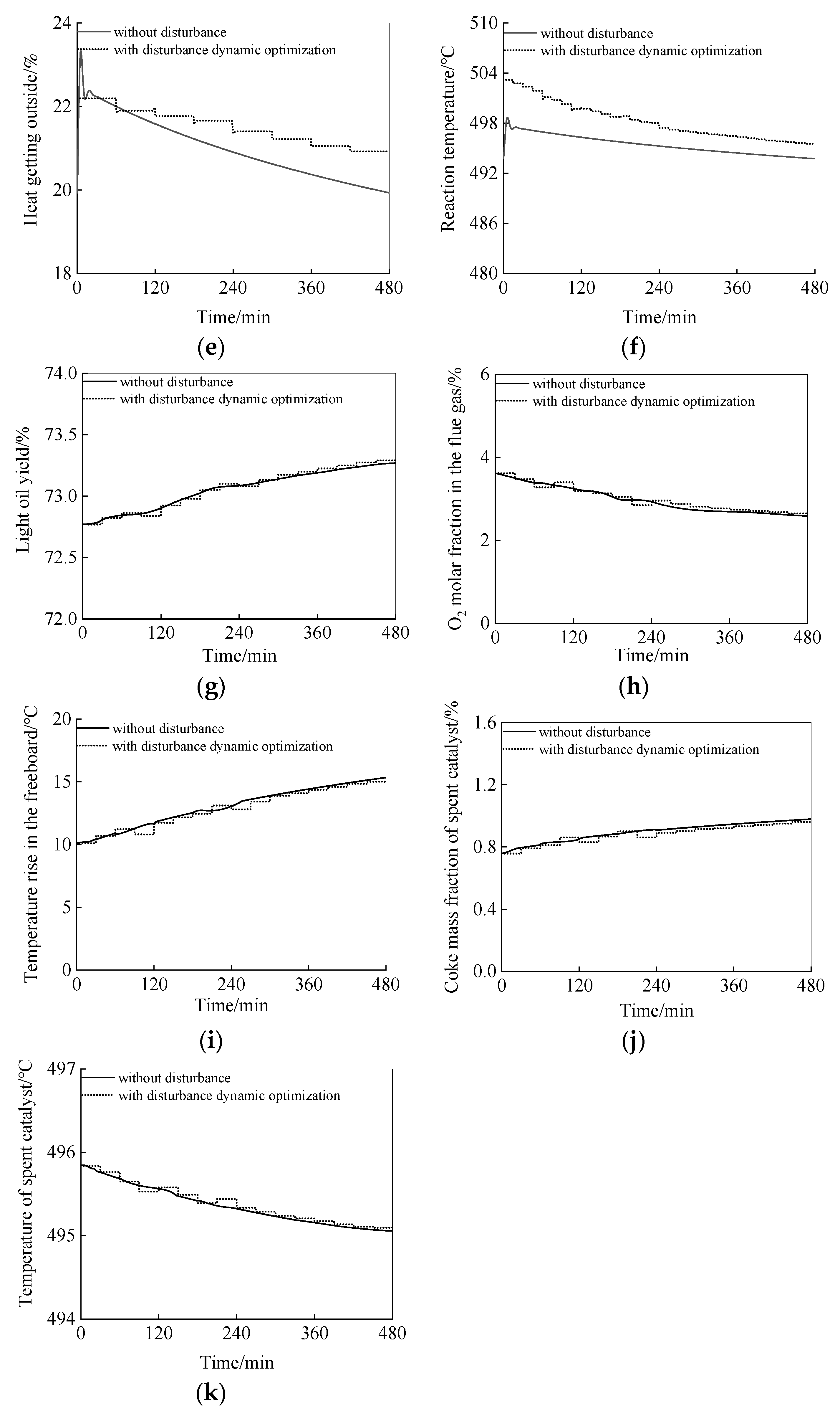
FCCU is in dynamic balance during stable operation. Due to unpredictable uncertainties when the system is running, there must be some external disturbance. Because the feed flow rate has more uncertainties, the feed flow rate is selected as the main disturbance factor. In order to study the dynamic performance of the multi-rate, variable-window online dynamic optimization method, disturbance is added for experimental comparative analysis. The experimental results are shown in Figure 9, and the composition of the objective function values is shown in Table 4.
The solid line in Figure 9 is the result of the experiment when there is no disturbance. The dotted line is the optimal solution obtained by adding disturbance in the standard case. It is found from Figure 9a that in order to ensure rationality before and after the comparison, the total amount of feedstock oil is kept unchanged. It can be seen from Figure 9b that multi-rate, variable-window online dynamic optimization can effectively improve the utilization rate of CO combustion promoters. When the feedstock amount decreases, the addition amount of CO combustion promoters decreases. It is found in Figure 9c that the amount of recycled slurry is higher than that before optimization because multi-rate, variable-window online dynamic optimization increases the utilization rate of safety margin space, thus promoting the conversion rate of feedstock oil. It can be seen from Figure 9d–f that due to the increase in the amount of recycled slurry, the coke-burning intensity in the system increases, and the reaction temperature increases, resulting in an increase in the heat escaping and the utilization rate of combustion air increases. It can be seen from Figure 9g that the light oil yield increases with increasing feed amount, and the light oil yield decreases with decreasing feed amount. In addition, the light oil yield can be effectively improved by multi-rate, variable-window dynamic optimization. This is because, in the optimization process, the time is divided to make the operating state of the system closer to the optimal operating point. Although the disturbance will affect the light oil yield, the overall trend remains unchanged. Figure 9h shows that with the decrease in the amount of feedstock oil added, the coke-burning intensity decreases, and the oxygen consumption decreases, resulting in the increase of oxygen content in the flue gas. The device adopts multi-rate, variable-window dynamic optimization, which improves the utilization rate of the incoming combustion air and increases the oxygen content in the flue gas. Although the disturbance will affect the optimization effect at a certain moment, the overall trend of the optimization result remains unchanged. It can be seen from Figure 9i that due to the decrease in feedstock oil, the coke-burning strength is weakened, which leads to a decrease in temperature in the dilute phase. Dynamic optimization increases the oxygen utilization rate and promotes temperature reduction in the dilute phase under the action of excessive combustion air. In Figure 9j, due to the high carbon residual value of the feedstock oil, the change in the addition amount will directly affect the coke mass fraction of the spent catalyst. With the increase in the added amount, the coke-burning strength increases and the coke content decreases. The multi-rate, variable-window dynamic optimization can effectively improve the working characteristics of the system, thus promoting the reduction in coke mass fraction on spent catalysts. In Figure 9k, due to the high carbon residue value of the feedstock oil, the feed amount is reduced, resulting in the weakening of coke-burning strength, and the temperature of the spent catalyst is decreased. The dynamic optimization improves the utilization rate of oxygen, promotes the coke-burning reaction, and causes the reaction temperature to increase. Through the above comparison experiments, it can be seen that, in the online dynamic optimization process, the addition of disturbance will have a direct impact on the optimization effect. However, during the whole optimization period, the changing trend of the experimental results remains unchanged, and only limited volatility is generated under the action of disturbance factors. This also just shows that multi-rate, variable-window online dynamic optimization has good dynamic performance and has a certain application value.
6. Conclusions
In this paper, a continuous chemical process based on multi-rate, variable-window online dynamic optimization was studied, taking FCCU with an external catalyst cooler as an example. First, heavy oil FCCU model expansion and multi-rate, variable-window online optimization analysis were carried out. Then, the single-rate, single-window CVP method and single-rate multi-window CVP method were analyzed, and the above methods were applied to the FCCU for simulation. In order to improve the practicability of optimization, a multi-rate, variable-window online dynamic optimization method was proposed. Then, the online dynamic optimization process of a multi-rate, variable-window system was analyzed by a mathematical method. Next, the online dynamic solution process of multi-rate, variable-window problem and the dynamic performance of multi-rate, variable-window dynamic optimization were studied. Multi-rate, variable-window online dynamic optimization can make the working state of the system closer to the optimal working point and improve the working efficiency of the system. Through analysis of the complex chemical system, CO combustion promoters, recycle slurry flow rate, combustion air flow rate, heat escape, and reaction temperature were taken as optimization variables. Therefore, for systems with two or more operating frequencies, a multi-rate, variable-window online dynamic optimization scheme was used to determine the optimal operating variables and active constraints. Finally, the experimental results proved the feasibility of the proposed multi-rate, variable-window online dynamic optimization in complex chemical systems and obtained ideal economic benefits while ensuring the steady operation of the system.
Author Contributions
Conceptualization, J.Z.; methodology, J.Z. and X.L.; software, J.Z., J.L., and F.X.; validation, J.Z., J.L., and F.X.; formal analysis, J.Z.; investigation, J.Z.; resources, J.Z. and X.L.; data curation, J.L. and F.X.; writing—original draft preparation, J.Z.; writing—review and editing, J.Z., J.L., and F.X.; visualization, J.Z.; supervision, X.L.; project administration, J.L., F.X., and X.L.; funding acquisition, X.L. All authors have read and agreed to the published version of the manuscript.
Funding
This research received no external funding.
Data Availability Statement
The data presented in this study are available on request from the corresponding author.
Acknowledgments
This work was supported by the National Natural Science Foundation of China (21676295).
Conflicts of Interest
The authors declare no conflict of interest.
Nomenclature
| Symbols | |
| A | area, m2 |
| C | coke content of catalysts, % |
| Cp | heat capacity, kJ/(kg·°C) |
| dp | average particle size of catalyst, m |
| D | diffusion coefficient, m2/s |
| DT | combustor diameter, m |
| E | activation energy, kJ/mol |
| F | mass flow rate, t/h |
| G | catalyst circulation rate, kg/s |
| h | film heat transfer coefficient, W/(m2·°C) |
| H | hydrogen content of catalysts, % |
| k | rate coefficient of a reaction or mass transfer rate coefficient |
| K | heat transfer coefficient |
| m | integer constant |
| M | mass flow rate, kg/s |
| N | constant coefficient |
| Nu | Nusselt number |
| O | cross-sectional area, m2 |
| P | pressure, Pa |
| Pe | Peclect number |
| Qs | total heat release, kJ/s |
| R | ideal gas constant, kJ/(mol·°C) |
| Rg | gas molar flux, mol/(m2·s) |
| Rtotal | catalyst mass flux, kg/(m2·s) |
| S | heat transfer area, m2 |
| T | temperature, °C |
| uf | linear velocity, m/s |
| V | gas flow rate, m3/s |
| W | inventory, t |
| xpro | amount of added CO combustion promoters, % |
| y | product yield or gas content, % |
| ZT | combustor length, m |
| Greek Letters | |
| β | carbon residue is converted to additional carbon, kg/kg |
| ΔH | reaction enthalpy, kJ/kg or kJ/mol |
| ΔT1 | temperature difference between Trg1 and saturated steam |
| ΔT2 | temperature difference between Trg2 and saturated steam |
| ΔT | log mean temperature difference, °C |
| ΔTf | temperature rise in the dilute phase, °C |
| ΔTw | coke-burning tank heat dissipation temperature difference, °C |
| γ | latent heat of vaporization of saturated water, kJ/kg |
| ε | Porosity |
| η | hydrogen−carbon molar ratio, H/C |
| η0 | heat extraction ratio, % |
| λg | axial thermal conductivity of gas, W/(m·K) |
| ρ | density, kg/m3 or mol/m3 |
| Subscripts and Superscripts | |
| C | coke |
| d | membrane |
| fresh | feedstock oil |
| g | gas phase |
| h | heat |
| hco | recycle oil |
| H | hydrogen |
| pro | combustion promoters |
| rg1 | combustor |
| rg2 | dense bed |
| rg3 | catalyst cooler |
| riser | reaction temperature |
| s | solid phase |
| sc | spent catalyst |
| slurry | recycle slurry |
| st | stripper |
| w | water or wall |
| ′0 | average after mixing |
| ′rg2 | external catalyst cooler output temperature |
| 1 | water vapor or inside |
| 2 | fluidizing air or outside |
Appendix A. Some Important Operating Parameters of FCCU
| Parameters | Value | Units |
| dense phase length, Lrg2 | 16 | m |
| external catalyst cooler height, Hs | 7.5 | m |
| reactor cross-sectional area, Ora | 0.636 | m2 |
| riser length, xt | 32 | m |
| wear-resistant heat-resistant layer density, ρi | 1845 | kg/m3 |
| cross-sectional area of coke-burning tank, Org1 | 19.63 | m2 |
| height of coke-burning tank, zt | 9.81 | m |
| coke-burning tank diameter, Dt | 5 | m |
| cross-sectional area of dense bed, Org2 | 9.23 | m2 |
| equivalent heat dissipation area of dense bed, Arg2 | 240.745 | m2 |
| total length of heat pipe, LT | 14 | m |
| catalyst particle density, ρs | 823.5 | kg/m3 |
| cross-sectional area of dilute phase, Od | 38.46 | m2 |
| part of carbon residue converted to additional carbon in feedstock oil, β | 0.6 | kg/kg |
| hydrogen−carbon molar ratio, η | 8/92 | kg/kg |
Appendix B. Research on Accounting Process
The external catalyst cooler leads the hot catalyst out of the regenerator and then returns the cold catalyst to the regenerator so as to achieve the purpose of extracting excess heat and controlling the temperature of the regenerator. The advantage of the external catalyst cooler is that the heat load can be adjusted, and the external catalyst cooler can be deactivated or activated at any time. The heat balance calculation of the external catalyst cooler is carried out, and the total heat release is Qs. The heat release of the external catalyst cooler is as follows:
The heat absorbed by the external catalyst cooler is
The heat transfer equation is
Logarithmic temperature difference equation is
Heat transfer coefficient is
Heat transfer coefficient in the tube is
Heat transfer coefficient outside the tube is
The model equations of carbon content and hydrogen content on the catalyst in the coke-burning tank are as follows. Among them, Rtotal contains three parts of the catalyst mass flow rate, which are the mass flow rate in the inclined tube to be grown, the mass flow rate from the dense bed to the coke-burning tank, and the mass flow rate of the internal circulation.
The ordinary differential equation of oxygen content in flue gas is as follows:
The regenerated catalyst exchanges heat through the external catalyst cooler to achieve the purpose of cooling the regenerated catalyst. This is not only beneficial to improving COR and conversion rate but also has a protective effect on the safe operation of the device. The heat calculation formula is as follows:
Through the operation of an external catalyst cooler, the cold catalyst is returned to the regenerator. Calculation of the temperature, carbon content, and hydrogen content of the catalyst after mixing in the coke-burning tank is as shown in the following equations.
For the material balance calculation of the second dense bed, the model equations for carbon content on the catalyst, the oxygen content in flue gas, and the reaction temperature are as follows.
References
- Biegler, L.T. An overview of simultaneous strategies for dynamic optimization. Chem. Eng. Process. Process Intensif. 2007, 46, 1043–1053. [Google Scholar] [CrossRef]
- Biegler, L.T.; Cervantes, A.M.; Wachter, A. Advances in simultaneous strategies for dynamic process optimization. Chem. Eng. Sci. 2002, 57, 575–593. [Google Scholar] [CrossRef]
- Zhang, Y.D.; Mo, Y.B. Dynamic Optimization of Chemical Processes Based on Modified Sailfish Optimizer Combined with an Equal Division Method. Processes 2021, 9, 1806. [Google Scholar] [CrossRef]
- Schlegel, M.; Stockmann, K.; Binder, T.; Marquardt, W. Dynamic optimization using adaptive control vector parameterization. Comput. Chem. Eng. 2005, 29, 1731–1751. [Google Scholar] [CrossRef]
- Kameswaran, S.; Biegler, L.T. Simultaneous dynamic optimization strategies: Recent advances and challenges. Comput. Chem. Eng. 2006, 30, 1560–1575. [Google Scholar] [CrossRef]
- Asgari, S.A.; Pishvaie, M.R. Dynamic optimization in chemical processes using region reduction strategy and control vector parameterization with an ant colony optimization algorithm. Chem. Eng. Technol. 2008, 31, 507–512. [Google Scholar] [CrossRef]
- Chen, X.; Du, W.L.; Tianfield, H.; Qi, R.B.; He, W.L.; Qian, F. Dynamic optimization of industrial processes with nonuniform discretization-based control vector parameterization. IEEE Trans. Autom. Sci. Eng. 2014, 11, 1289–1299. [Google Scholar] [CrossRef]
- Zhang, Y.H.; Chen, G.X.; Yan, G.S.; Li, B.; Lu, J.; Jiang, W. Multi-Objective Optimization of Kinetic Characteristics for the LBPRM-EHSPCS System. Processes 2023, 11, 2623. [Google Scholar] [CrossRef]
- Hartwich, A.; Marquardt, W. Dynamic optimization of the load change of a large-scale chemical plant by adaptive single shooting. Comput. Chem. Eng. 2010, 34, 1873–1889. [Google Scholar] [CrossRef]
- De Prada, C.; Mazaeda, R.; Podar, S. Optimal operation of a combined continuous–batch process. Comput. Aid. Chem. Eng. 2018, 44, 673–678. [Google Scholar]
- Ding, F.; Chen, T.W. Modeling and identification of multirate systems. Act. Auto. Sin. 2005, 31, 105–122. [Google Scholar]
- Arandes, J.M.; Torre, I.; Azkoiti, M.J.; Erena, J.; Bilbao, J. Effect of atmospheric residue incorporation in the fluidized catalytic cracking (FCC) feed on product stream yields and composition. Energy Fuels 2008, 22, 2149–2156. [Google Scholar] [CrossRef]
- Chen, L.H.; Cheng, M.Z.; Cai, Y.; Guo, L.; Gao, D. Multi−Objective Collaborative Optimization Design of Key Structural Parameters for Coal Breaking and Punching Nozzle. Processes 2022, 10, 1036. [Google Scholar] [CrossRef]
- Harding, R.H.; Peters, A.W.; Nee, J.R.D. New developments in FCC catalyst technology. Appl. Catal. A 2001, 221, 389–396. [Google Scholar] [CrossRef]
- Spretz, R.; Sedran, U. Operation of FCC with mixtures of regenerated and deactivated catalyst. Appl. Catal. A 2001, 215, 199–209. [Google Scholar] [CrossRef]
- Devard, A.; Puente, G.; Passamonti, F.; Sedran, U. Processing of resid–VGO mixtures in FCC: Laboratory approach. Appl. Catal. A 2009, 353, 223–227. [Google Scholar] [CrossRef]
- Srinivasan, B.; Palanki, S.; Bonvin, D. Dynamic optimization of batch processes: I. Characterization of the nominal solution. Comput. Chem. Eng. 2003, 27, 1–26. [Google Scholar] [CrossRef]
- Xu, Y.H.; Zhang, J.S.; Long, J.; He, M.Y.; Xu, H.; Hao, X.R. Development and commercial application of FCC process for maximizing iso-paraffins (MIP) in cracked naphtha. Eng. Sci. 2003, 5, 55–58. [Google Scholar]
- Ancheyta, J.J.; Lopez, F.I.; Aguilar, E.R. Correlations for predicting the effect of feedstock properties on catalytic cracking kinetic parameters. Ind. Eng. Chem. Res. 1998, 37, 4637–4640. [Google Scholar] [CrossRef]
- Ancheyta, J.J.; Lopez, F.I.; Aguilar, E.R. 5-Lump kinetic model for gas oil catalytic cracking. Appl. Catal. A 1999, 177, 227–235. [Google Scholar] [CrossRef]
- Wang, H.; Sheng, B.; Lu, Q.; Yin, X.; Zhao, F.; Lu, X.; Luo, R.; Fu, G. A novel multi-objective optimization algorithm for the integrated scheduling of flexible job shops considering preventive maintenance activities and transportation processes. Soft Comput. 2021, 25, 2863–2889. [Google Scholar] [CrossRef]
- Ancheyta, J.J.; Lopez, F.I.; Aguilar, E.R. A strategy for kinetic parameter estimation in the fluid catalytic cracking process. Ind. Eng. Chem. Res. 1997, 36, 5170–5174. [Google Scholar] [CrossRef]
- Otterstedt, J.E.; Gevert, S.B.; Jas, S.G.; Menon, P.G. Fluid catalytic cracking of heavy (residual) oil fractions: A review. Appl. Catal. 1986, 22, 159–179. [Google Scholar] [CrossRef]
- Ahmadi, E.; Zandieh, M.; Farrokh, M.; Emami, S.M. A multi objective optimization approach for flexible job shop scheduling problem under random machine breakdown by evolutionary algorithms. Comput. Oper. Res. 2016, 73, 56–66. [Google Scholar] [CrossRef]
- Chu, Y.; You, F. Integrated Scheduling and Dynamic Optimization of Complex Batch Processes with General Network Structure Using a Generalized Benders Decomposition Approach. Ind. Eng. Chem. Res. 2013, 52, 7867–7885. [Google Scholar] [CrossRef]
- Nie, Y.; Biegler, L.T.; Villa, C.M.; Wassick, J.M. Discrete time formulation for the integration of scheduling and dynamic optimization. Ind. Eng. Chem. Res. 2015, 54, 4303–4315. [Google Scholar] [CrossRef]
- Wu, Y.C.; Sun, G.; Tao, J. An Improved Multi-Objective Particle Swarm Optimization Method for Rotor Airfoil Design. Aerospace 2023, 10, 820. [Google Scholar] [CrossRef]
- Li, R.; Chen, Y.L.; Song, J.Z.; Li, M.; Yu, Y. Multi-Objective Optimization Method of Industrial Workshop Layout from the Perspective of Low Carbon. Sustainability 2023, 15, 12275. [Google Scholar] [CrossRef]
- Zhang, X.; Zhang, G.Y.; Zhang, D.; Zhang, L.; Qian, F. Dynamic Multi-Objective Optimization in Brazier-Type Gasification and Carbonization Furnace. Materials 2023, 16, 1164. [Google Scholar] [CrossRef]
- Hu, Q.; Zhai, X.Y.; Li, Z.F. Multi-Objective Optimization of Deep-Sea Mining Pump Based on CFD, GABP Neural Network and NSGA-III Algorithm. J. Mar. Sci. Eng. 2022, 10, 1063. [Google Scholar] [CrossRef]
- Hu, H.G.; Xu, L.H.; Wei, R.H.; Zhu, B. Multi-Objective Control Optimization for Greenhouse Environment Using Evolutionary Algorithms. Sensors 2011, 11, 5792–5807. [Google Scholar] [CrossRef] [PubMed]
- Ke, W.L.; Sha, J.H.; Yan, J.J.; Zhang, G.; Wu, R. A Multi-Objective Input–Output Linear Model for Water Supply, Economic Growth and Environmental Planning in Resource-Based Cities. Sustainability 2016, 8, 160. [Google Scholar] [CrossRef]
- Quan, Z.; Wang, Y.; Ji, Z. Multi-objective optimization scheduling for manufacturing process based on virtual workflow models. Appl. Soft Comput. 2022, 122, 108786. [Google Scholar] [CrossRef]
- Arbel, A.; Huang, Z.; Rinard, I.H.; Shinnar, R.; Sapre, A.V. Dynamic and Control of Fluidized Catalytic Crackers. 1. Modeling of the Current Generation of FCC’s. Ind. Eng. Chem. Res. 1995, 34, 1228–1243. [Google Scholar] [CrossRef]
- Lin, J.J.; Xu, F.; Luo, X. Dynamic Optimization of Continuous-Batch Processes: A Case Study of an FCCU with CO Promoter. Ind. Eng. Chem. Res. 2019, 58, 23187–23200. [Google Scholar] [CrossRef]
- Wang, M.C.; Li, Y.J.; Yuan, J.P.; Osman, F.K. Matching Optimization of a Mixed Flow Pump Impeller and Diffuser Based on the Inverse Design Method. Processes 2021, 9, 260. [Google Scholar] [CrossRef]
- Nie, Y.; Biegler, L.T.; Wassick, J.M. Integrated scheduling and dynamic optimization of batch processes using state equipment networks. AICHE J. 2012, 58, 3416–3432. [Google Scholar] [CrossRef]
- Weng, J.Z.; Shao, Z.J.; Chen, X.; Gu, X.P.; Yao, Z.; Feng, L.F.; Biegler, L.T. A novel strategy for dynamic optimization of grade transition processes based on molecular weight distribution. AIChE J. 2014, 60, 2498–2512. [Google Scholar] [CrossRef]
- Prata, A.; Oldenburg, J.; Kroll, A.; Marquardt, W. Integrated scheduling and dynamic optimization of grade transitions for a continuous polymerization reactor. Comput. Chem. Eng. 2008, 32, 463–476. [Google Scholar] [CrossRef]
- Morison, K.R.; Sargent, R.W.H. Optimization of multistage processes described by differential-algebraic equations. In Numerical Analysis; Springer: Berlin/Heidelberg, Germany, 1986; pp. 86–102. [Google Scholar]
- Liu, R.; Li, J.; Liu, J.; Jiao, L. A survey on dynamic multi-objective optimization. Chin. J. Comput. 2020, 43, 1246–1278. [Google Scholar]
- Binder, T.; Cruse, A.; Villar, C.A.C.; Marquardt, W. Dynamic optimization using a wavelet based adaptive control vector parameterization strategy. Comput. Chem. Eng. 2000, 24, 1201–1207. [Google Scholar] [CrossRef]
- Wongrat, W.; Younes, A.; Elkamel, A.; Douglas, P.L.; Lohi, A. Control vector optimization and genetic algorithms for mixed-integer dynamic optimization in the synthesis of rice drying processes. J. Franklin. Inst. 2011, 348, 1318–1338. [Google Scholar] [CrossRef]
- Luo, Z.Y.; Tan, S.X.; Liu, X.T.; Xu, H.; Liu, J. Multi-Objective Workflow Optimization Algorithm Based on a Dynamic Virtual Staged Pruning Strategy. Processes 2023, 11, 1160. [Google Scholar] [CrossRef]
- Zhang, P.P.; Chen, H.M.; Liu, X.G.; Zhang, Z.Y. An iterative multi-objective particle swarm optimization-based control vector parameterization for state constrained chemical and biochemical engineering problems. Biochem. Eng. J. 2015, 103, 138–151. [Google Scholar] [CrossRef]
- Pili, R.; Jørgensen, B.J.; Haglind, F. Multi-objective optimization of organic Rankine cycle systems considering their dynamic performance. Energy 2022, 246, 123345. [Google Scholar] [CrossRef]
- Zhang, J.; Shen, Y.; Gan, M.; Su, Q.; Lyu, F.; Xu, B.; Chen, Y. Multi-objective optimization of surface texture for the slipper/swash plate interface in EHA pumps. Front. Mech. Eng. 2022, 17, 48. [Google Scholar] [CrossRef]
- Zhang, J.F.; Lin, J.; Luo, X.; Xu, F. Modeling analysis for product distribution control and optimization of heavy oil FCCU. CIESC J. 2022, 73, 1232–1245. [Google Scholar]
Figure 1.
Schematic diagram of FCCU with external catalyst cooler [48].
Figure 1.
Schematic diagram of FCCU with external catalyst cooler [48].
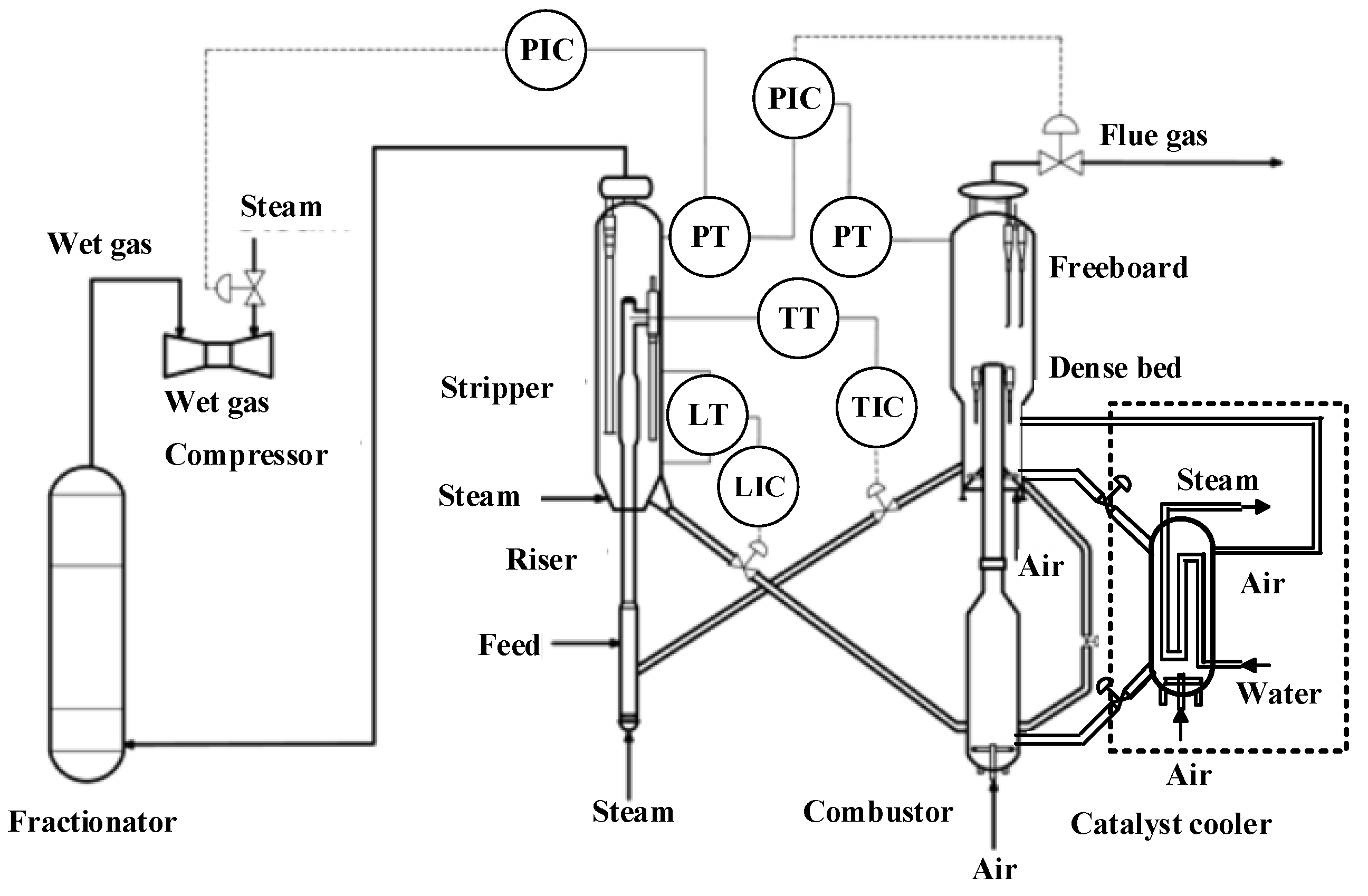
Figure 2.
Research on single-rate multi-window CVP method.

Figure 3.
Flow chart of multi-rate, variable-window system dynamic optimization process.

Figure 4.
Research on online dynamic optimization process of multi-rate, variable-window system.
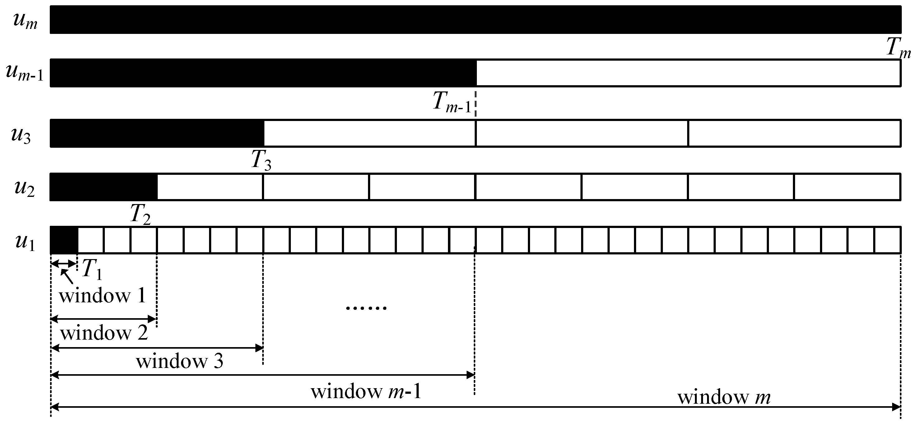
Figure 5.
Multi-rate, variable-window online dynamic optimization solution process.
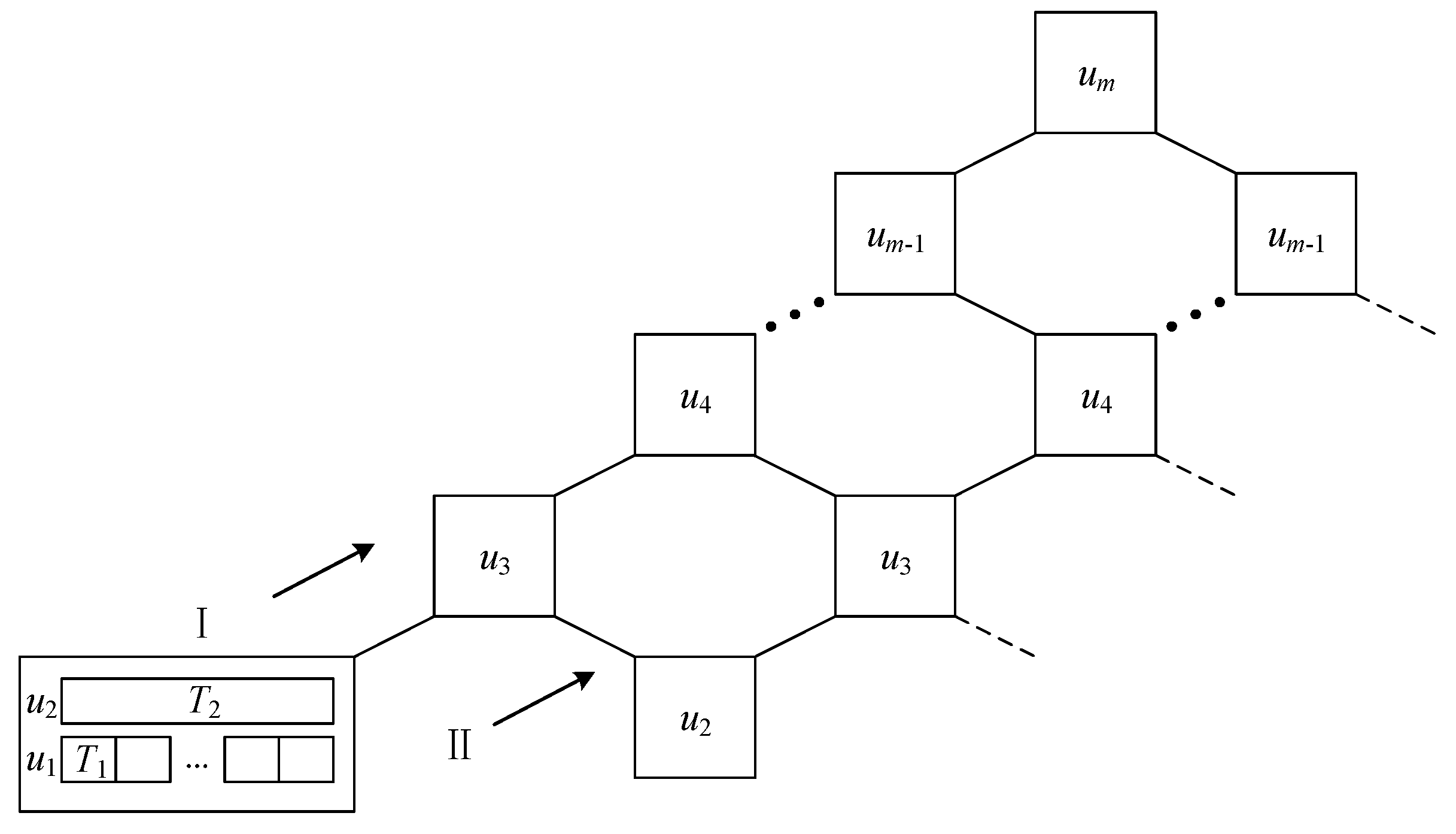
Figure 6.
Dynamic characteristics of the system under nominal operating conditions: (a) temperature of spent catalyst, (b) coke mass fraction of spent catalyst, (c) temperature rise in the freeboard, (d) O2 molar fraction in the flue gas, (e) COR, and (f) light oil yield.
Figure 6.
Dynamic characteristics of the system under nominal operating conditions: (a) temperature of spent catalyst, (b) coke mass fraction of spent catalyst, (c) temperature rise in the freeboard, (d) O2 molar fraction in the flue gas, (e) COR, and (f) light oil yield.
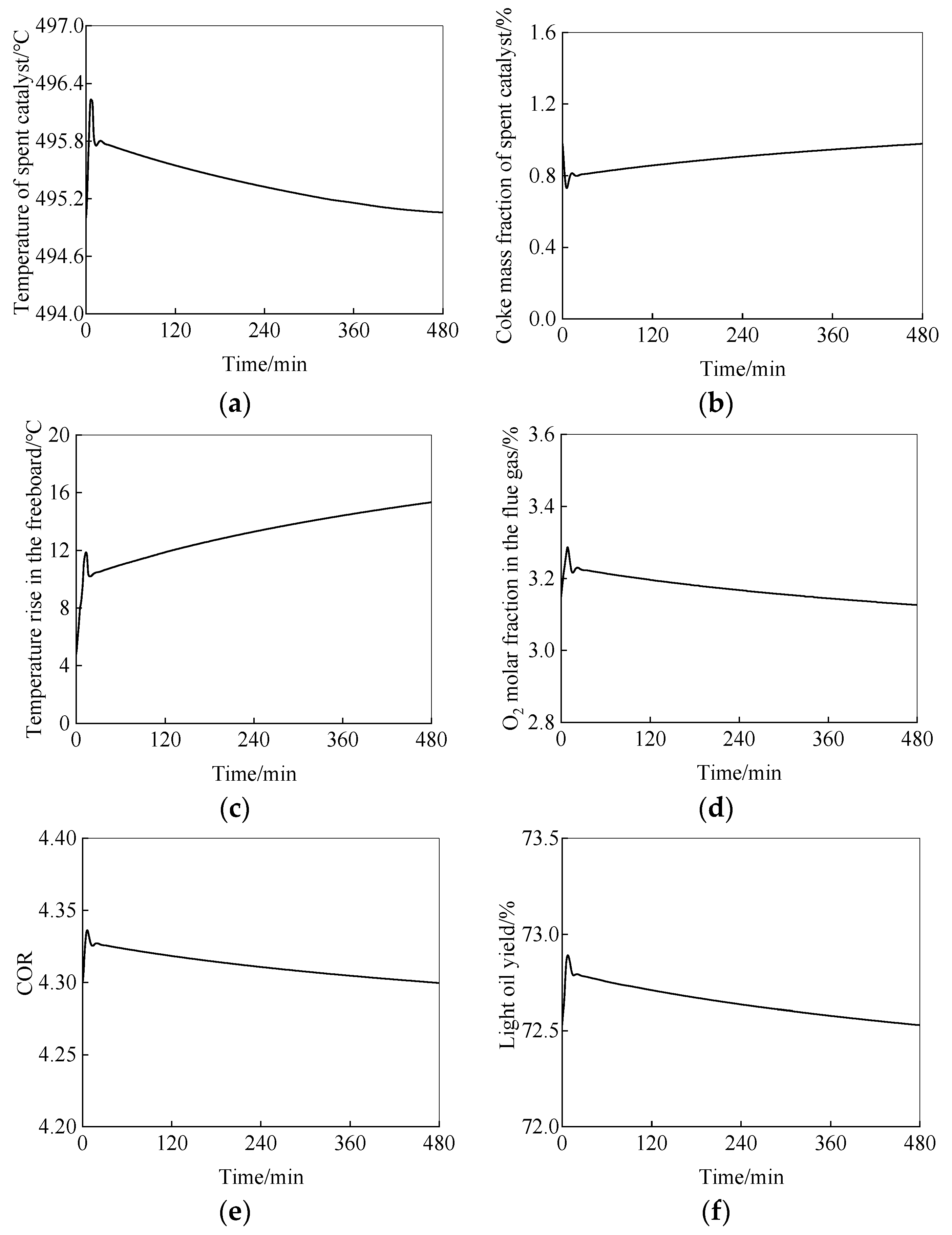
Figure 7.
Sensitivity analysis of different dynamic optimization methods: (a) CO combustion promoters, (b) recycle slurry, (c) combustion air flow rate, (d) heat escape, and (e) reaction temperature of riser.
Figure 7.
Sensitivity analysis of different dynamic optimization methods: (a) CO combustion promoters, (b) recycle slurry, (c) combustion air flow rate, (d) heat escape, and (e) reaction temperature of riser.
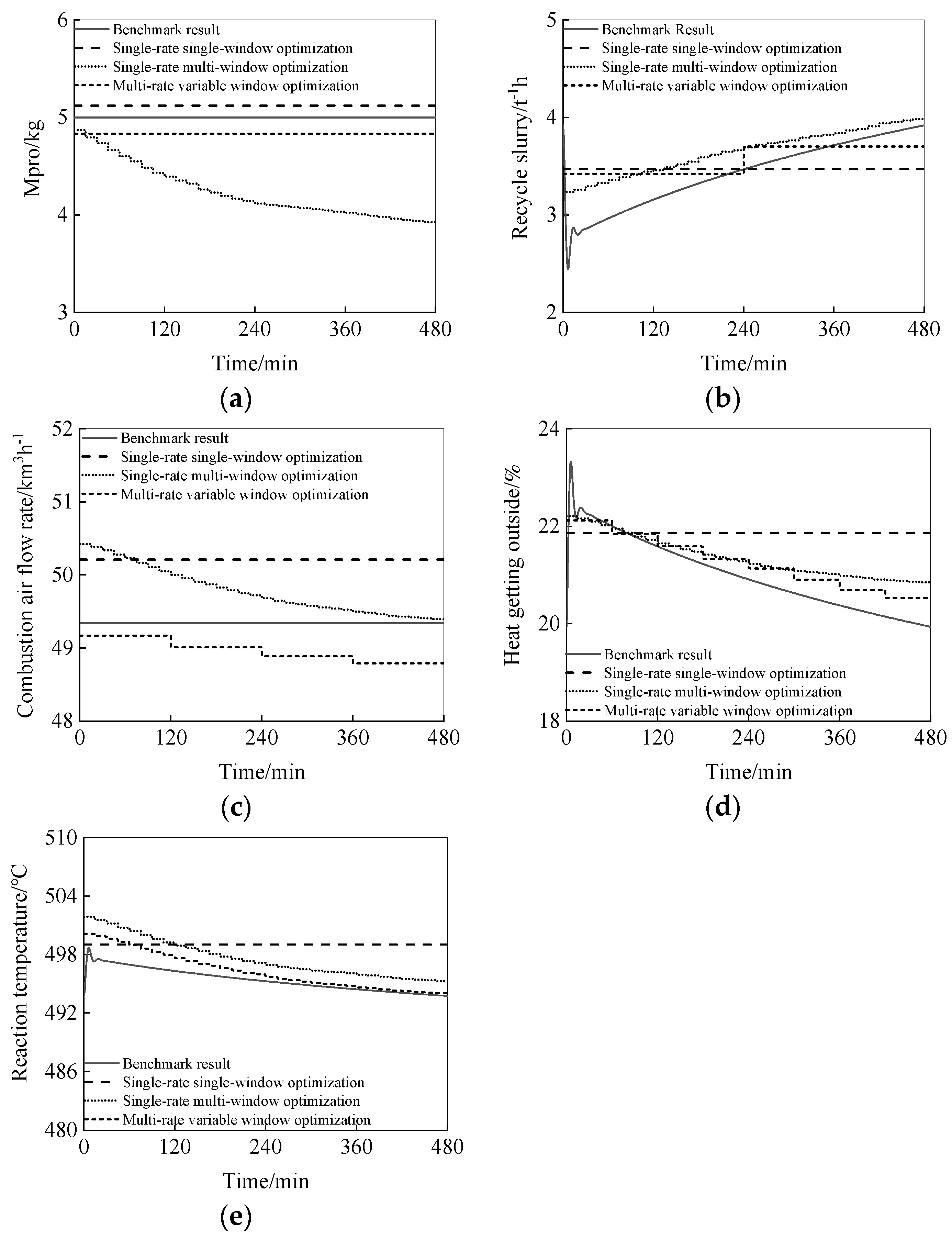
Figure 8.
Sensitivity analysis of different dynamic optimization to light oil yield.
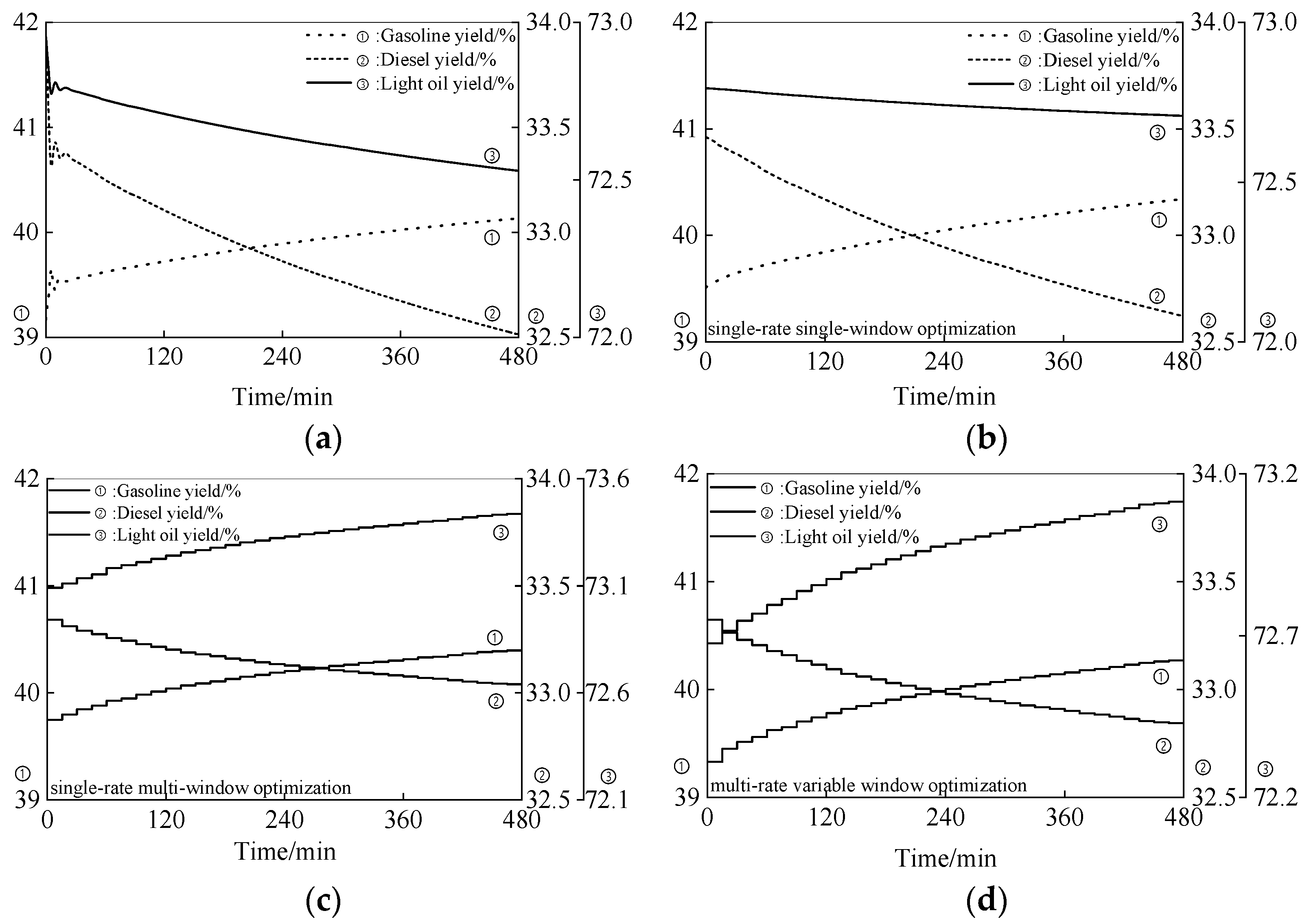
Figure 9.
Comparative analysis of experiments with disturbance: changes in target variables and some important parameters.
Figure 9.
Comparative analysis of experiments with disturbance: changes in target variables and some important parameters.


Table 1.
Change in optimization variables.
| Time | Optimization Variables | Variables |
|---|---|---|
| [0, T2] | u1 | u2, u3, …, um |
| [T2, T3] | u1, u2 | u3, u4, …, um |
| [T3, T4] | u1, u2, u3 | u4, u5, …, um |
| … | … | … |
| [Tm−1, Tm] | u1, u2, …, um−1 | um |
Table 2.
FCCU base case operating conditions.
| Variables | Value | Units |
|---|---|---|
| fresh feed flow rate, Ffresh | 85 | t/h |
| HCO flow rate, Fhco | 12.75 | t/h |
| regenerated catalyst circulation rate, Grg2 | 504.2 | t/h |
| catalyst-to-oil ratio, COR | 4.31 | wt/wt |
| combustion air flow rate, Vrg1 | 49,340 | m3/h |
| fluffing air flow rate, Vrg2 | 6658 | m3/h |
| amount of added CO combustion promoters, Mpro | 5 | kg |
| concentration of CO combustion promoters, xpro | 0.005 | wt% |
| inventories, W (combustor/dense bed/stripper) | 24/5/5 | t |
| reaction temperature, Triser | 495.4 | °C |
| recycle slurry flow rate, Fslurry | 3.35 | t/h |
| heat getting outside ratio, η0 | 21 | % |
| combustor top temperature, Trg1 | 698.6 | °C |
| dense bed temperature, Trg2 | 707.3 | °C |
| coke content of spent catalysts, Csc | 0.97 | wt% |
| coke content of regenerated catalysts, Crg2 | 0.045 | wt% |
| O2 content in flue gas, yO2 | 3.17 | mol% |
| CO content in flue gas, yCO | 0.15 | mol% |
| CO2 content in flue gas, yCO2 | 13.85 | mol% |
Table 3.
Constraints of operating variables and state variables.
| Variables | Lower Bound | Upper Bound |
|---|---|---|
| reaction temperature, Triser (°C) | 490 | 510 |
| dense bed temperature, Trg2 (°C) | 680 | 725 |
| coke content of spent catalysts, Csc (wt%) | 0.5 | 1.2 |
| O2 content in flue gas, yO2 (mol%) | 3 | 4 |
| yield of coke, yc (wt%) | 8 | 10.7 |
| yield of diesel, yd (wt%) | 32 | 34 |
| yield of gasoline, yn (wt%) | 39 | 41 |
| yield of wet gas, yg (wt%) | 10 | 20 |
| temperature rise in the freeboard, ΔTf (°C) | −5 | 20 |
| combustion air flow rate, Vrg1 (km3/h) | 40 | 55 |
| amount of added CO promoters, Mpro (kg) | 2 | 7 |
| recycle slurry flow rate, Fslurry (t/h) | 0 | 7.25 |
| combustor top temperature, Trg1 (°C) | 660 | 695 |
| heat escape ratio, η0 (%) | 0 | 30 |
| light oil yield, y (wt%) | 71 | 75 |
Table 4.
Detailed composition of economic benefits of different operating models.
| Variables | Gasoline | Diesel | Slurry | CO Combustion Promoters | Combustion Air | Recycle Slurry Energy Consumption | Heat Escape Energy Consumption | Flue Gas Energy | |
|---|---|---|---|---|---|---|---|---|---|
| benchmark operation | 271.014 | 223.829 | 0 | 5 | 1,449,792 | 58 | 0 | 3.17 × 10⁷ | |
| single-rate, single-window optimization period 8 h | dynamic optimization | 271.053 | 223.913 | 30.59 | 5.121 | 1,445,968 | 25.48 | 206.78 | 1.42 × 10⁷ |
| difference | 0.039 t | 0.084 t | 30.59 t | 0.121 kg | −3824 km3 | 25.48 km3 | 206.78 km3 | −1.75 × 10⁷ kJ | |
| benefits | 43.51$ | 79.77$ | 6162.35$ | 3.75$ | 11.19$ | 5.65$ | −45.88$ | −92.84$ | |
| total benefits | 6167.5$ | ||||||||
| single-rate, multi-window optimization period 15 min | dynamic optimization | 271.956 | 224.911 | 26.489 | 4.245 | 1,438,065 | 29.83 | 216.421 | 1.64 × 10⁷ |
| difference | 0.942 t | 1.082 t | 26.489 t | −0.755 kg | −11,727 km3 | 29.83 km3 | 216.421 km3 | −1.53 × 10⁷ kJ | |
| benefits | 1050.62$ | 1026.24$ | 5336.38$ | 23.41$ | 34.32$ | 6.62$ | −48.02$ | −81.17$ | |
| total benefits | 7348.4$ | ||||||||
| multi-rate, variable-window online dynamic optimization | dynamic optimization | 271.227 | 224.282 | 29.826 | 4.832 | 1,443,072 | 26.27 | 190.95 | 1.46 × 10⁷ |
| difference | 0.213 t | 0.453 t | 29.826 t | −0.168 kg | −6720 km3 | 26.27 km3 | 190.95 km3 | −1.71 × 10⁷ kJ | |
| benefits | 273.56$ | 429.65$ | 6008.65$ | 5.21$ | 19.67$ | 5.83$ | −42.37$ | −90.72$ | |
| total benefits | 6609.48$ | ||||||||
| multi-rate, variable-window online dynamic optimization (with disturbance) | dynamic optimization | 272.035 | 224.935 | 26.354 | 4.332 | 1,443,923 | 30.54 | 214.32 | 1.73 × 10⁷ |
| difference | 1.021 t | 1.106 t | 26.354 t | −0.668 kg | −5869 km3 | 30.54 km3 | 214.32 km3 | −1.44 × 10⁷ kJ | |
| benefits | 1311.29$ | 1048.99$ | 5309.19$ | 20.72$ | 17.18$ | 6.77$ | −47.56$ | −76.39$ | |
| total benefits | 7590.19$ | ||||||||
Disclaimer/Publisher’s Note: The statements, opinions and data contained in all publications are solely those of the individual author(s) and contributor(s) and not of MDPI and/or the editor(s). MDPI and/or the editor(s) disclaim responsibility for any injury to people or property resulting from any ideas, methods, instructions or products referred to in the content. |
© 2023 by the authors. Licensee MDPI, Basel, Switzerland. This article is an open access article distributed under the terms and conditions of the Creative Commons Attribution (CC BY) license (https://creativecommons.org/licenses/by/4.0/).
Share and Cite
MDPI and ACS Style
Zhang, J.; Lin, J.; Xu, F.; Luo, X. Online Dynamic Optimization of Multi-Rate Processes with the Case of a Fluid Catalytic Cracking Unit. Processes 2023, 11, 3088. https://doi.org/10.3390/pr11113088
AMA Style
Zhang J, Lin J, Xu F, Luo X. Online Dynamic Optimization of Multi-Rate Processes with the Case of a Fluid Catalytic Cracking Unit. Processes. 2023; 11(11):3088. https://doi.org/10.3390/pr11113088
Chicago/Turabian StyleZhang, Jianfei, Jiajiang Lin, Feng Xu, and Xionglin Luo. 2023. "Online Dynamic Optimization of Multi-Rate Processes with the Case of a Fluid Catalytic Cracking Unit" Processes 11, no. 11: 3088. https://doi.org/10.3390/pr11113088
Note that from the first issue of 2016, this journal uses article numbers instead of page numbers. See further details here.