
Heat and Mass Transfer to Particles in One-Dimensional Oscillating Flows

1
Boysen-TU Dresden-Research Training Group, Technische Universität Dresden, Chemnitzer Straße 48b, 01062 Dresden, Germany
2
Chair of Energy Process Engineering, Institute of Process Engineering and Environmental Technology, Technische Universität Dresden, George-Bähr-Straße 3b, 01069 Dresden, Germany
*
Author to whom correspondence should be addressed.
Processes 2023, 11(1), 173; https://doi.org/10.3390/pr11010173
Submission received: 5 December 2022
/
Revised: 2 January 2023
/
Accepted: 3 January 2023
/
Published: 5 January 2023
(This article belongs to the Special Issue Multiphase Flows and Particle Technology)
Abstract
:The heat and mass transfer to solid particles in one-dimensional oscillating flows are investigated in this work. A meta-correlation for the calculation of the Nusselt number (Sherwood number) is derived by comparing 33 correlations and data point sets from experiments and simulations. These models are all unified by their dependencies on the amplitude parameter and the Reynolds number , while the - plane is applied as a framework in order to graphically display the various models. This is the first study to consider this problem in the entire - plane quantitatively while taking preexisting asymptotic models for various areas of the - plane into account.
Keywords:
oscillating flow; heat transfer; mass transfer; one-dimensional; ϵ-Re plane; spheres; particles; correlation; meta1. Introduction
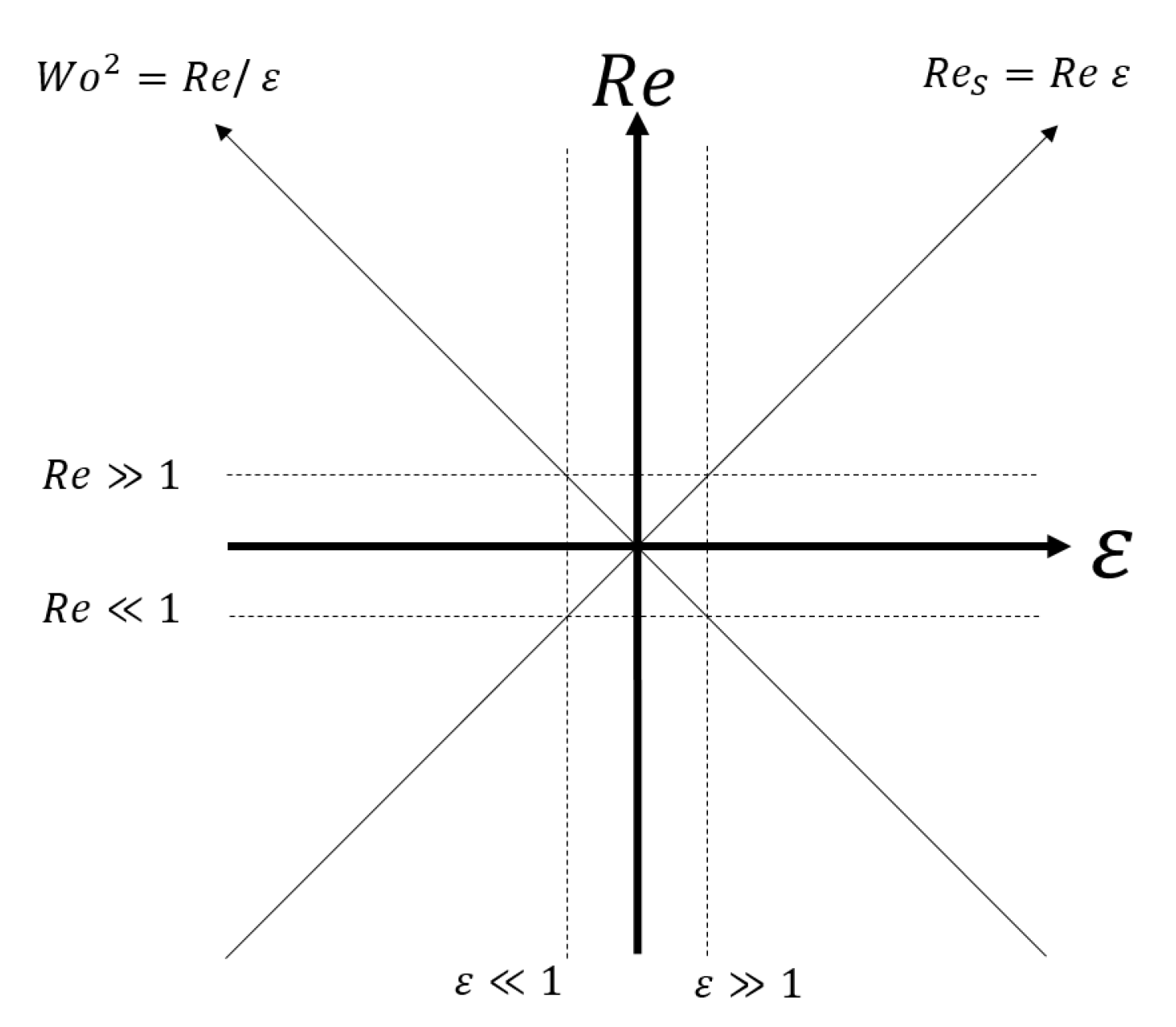
The heat and mass transfer (HMT) to (or from) a rigid, spherical particle suspended in a harmonically oscillating one-dimensional flow is considered. This configuration can be found, for example, in ultrasonic levitators [1,2] and pulsation reactors [3,4,5]. In case the particle is fixed in position (or the particle executes harmonic oscillations in a fluid at rest), the interaction between the fluid and the particle as well as the resulting flow state is defined by two dimensionless numbers: the particle Reynolds number and the amplitude parameter . The particle Reynolds number expresses the ratio between inertial and viscous forces with the slip velocity amplitude U, the density of the fluid , the particle diameter d, and the dynamic viscosity of the fluid . The amplitude parameter sets the particle displacement A in relation to the particle diameter, while the particle displacement itself is the ratio of slip velocity amplitude to the angular frequency of the oscillating fluid. An overview of these relations is provided in Appendix B. The Reynolds number and amplitude parameter span a plane in which all flow states can be pinpointed, as shown in Figure 1. The bisectors of this plane are the Womersley number [6], which is important for relaxation considerations, and the streaming Reynolds number [7], which is central for the modeling of steady streaming. Note that the origin of Figure 1 has the coordinates . The - plane was introduced by Wang [8] and then adopted by Chong et al. [9]. A comprehensive discussion of particle motion, particle relaxation and slip velocity in this configuration with the - plane as a basis was then conducted by Heidinger et al. [10]. Going forward, the - plane will simply be referred to as “plane” in this context. Not only is the particle motion and flow state of the described configuration defined by the two central dimensionless numbers and , but also the resulting heat and mass transfer. This means that pinpointing the location on the plane also delivers the intensity of the HMT from the particle. The intensity of the HMT is expressed via the Nusselt number or the Sherwood number , respectively. Many experimental and theoretical studies have already been conducted, but as they each cover only a small part of the plane, a comprehensive analysis of the HMT over the entire plane is still lacking. In the following, 33 data sets and correlations, each of which covers only a small part of the plane, are utilized in order to derive a meta-correlation, which covers the entire plane. In Section 2, an overview of the utilized works is presented, along with the general taxonomy and the approach adopted in this work. Then, in Section 3.1, the models for the quasi-steady sub-area of the plane are discussed and a steady meta-correlation is derived, which is later utilized for the general meta-correlation. The method for evaluating model deviations is introduced and the fit of the steady meta-correlation is evaluated. After that, Section 3.2 deals with data sets from oscillating flows, from which two general meta-correlations, one for fluid and one for gaseous environments, are derived. This is followed by a discussion of the design of the two meta-correlations in Section 4.1, and a discussion of the deviations between the meta-correlations and the utilized data sets in Section 4.2. Section 4.3 closes the discussion by evaluating the limits of the often applied quasi-steady assumption under the derived meta-correlations. The work is concluded with Section 5, in which the main features of the meta-correlations are highlighted.
2. Method
A Nusselt (Sherwood) number correlation for the entire plane is derived. For this purpose, a structured literature review is conducted in order to cover large parts of the plane with experimental, numerical, and analytical data for the occurring HMT. A list of the considered works can be found in Table 1 and a graphical overview in Figure 2. The Reynolds analogy (Prandtl analogy) is considered applicable in oscillating flows [9,11,12], leading to the interchangeability of correlations for Nusselt number and Sherwood number by exchanging the Schmidt number for the Prandtl number and vise versa. Therefore, the correlations for HMT to particles suggested by many authors can be expressed generally as
while the parameters () differ for individual correlations. For steady HMT, this approach has been used by Yavuzkurt et al. [12] and it is here extended with the term ‘’ in order to incorporate correlations for oscillating flows. All correlations in Table 1 fit this general ansatz except one.
Several authors concluded that, for a large enough amplitude parameter , the HMT in oscillating flow can be described by correlations for steady flow with sufficient accuracy. In these cases, the quasi-steady assumptions hold true.

Table 1.
A list of investigated works in the literature dealing with the HMT to spherical particles in steady (upper part) and oscillating flows (lower part).
Table 1.
A list of investigated works in the literature dealing with the HMT to spherical particles in steady (upper part) and oscillating flows (lower part).
| Authors | ( - ) | Steady (%) (Max) | Meta (%) (Max) | A | B | C | i | j | k | l | Source |
|---|---|---|---|---|---|---|---|---|---|---|---|
| Mori et al. | 4–24 | 8.4 (12.3) | 8.7 (15.1) | 2.000 | 0.550 | 0.000 | 0.500 | 0.000 | 0.333 | 0.000 | [13] |
| Ranz andMarshall | 0.1–2 × 10⁻² | 3.8 (10.3) | 3.8 (24.3) | 2.000 | 0.600 | 0.000 | 0.500 | 0.000 | 0.333 | 0.000 | [14] |
| Hsu et al. | 60–320 | 6.4 (9.0) | 8.4 (30.2) | 2.000 | 0.544 | 0.000 | 0.500 | 0.000 | 0.333 | 0.000 | [15] |
| Whitaker | 3.5–7.6 × 10⁴ | 7.0 (21.9) | 5.2 (46.1) | 2.000 | 0.400 | 0.060 | 0.500 | 0.667 | 0.400 | 0.000 | [16] |
| Gnielinski | 1–104 | 9.8 (32.9) | 7.2 (28.1) | 2.000 | 0.664 | 0.000 | 0.500 | 0.000 | 0.333 | 0.000 | [17] |
| Ke et al. | 10–200 | 9.7 (19.2) | 9.0 (21.7) | 1.910 | 0.545 | 0.019 | 0.500 | 0.667 | 0.333 | 0.000 | [18] |
| Richter and Nikrityuk | 10–250 | 6.9 (15.5) | 6.8 (24.6) | 1.760 | 0.550 | 0.014 | 0.500 | 0.667 | 0.333 | 0.000 | [19] |
| Sayegh and Gauvin | 0.2–100 | 3.4 (5.1) | 3.8 (28.3) | 2.000 | 0.473 | 0.000 | 0.552 | 0.000 | 0.780 | 0.000 | [20] |
| Melissari and Argyropoulos | 102–5 × 10⁴ | 2.9 (7.2) | 3.5 (36.7) | 2.000 | 0.470 | 0.000 | 0.500 | 0.000 | 0.360 | 0.000 | [21] |
| Witte | 3.5 × 10⁴–1.5 × 10⁵ | 26.2 (35.8) | 20.9 (72.2) | 2.000 | 0.386 | 0.000 | 0.500 | 0.000 | 0.500 | 0.000 | [22] |
| Chuchottaworn et al. | 1–200 | 7.8 (26.5) | 6.3 (23.4) | 2.000 | 0.370 | 0.000 | 0.610 | 0.000 | 0.510 | 0.000 | [23] |
| Bagchi et al. | 50–500 | 10.2 (15.1) | 11.7 (23.1) | data points—no given correlation | [24] | ||||||
| Blackburn | 1–100 | 6.0 (11.2) | 6.0 (13.8) | data points—no given correlation | [25] | ||||||
| Acrivos and Taylor | 0–1 | 6.4 (7.4) | 6.2 (14.0) | [26] | |||||||
| Steady meta-correlation | 10−1–1.5 × 10⁵ | 4.3 (27.1) | 1.7 (24.0) | 2.000 | 0.500 | 0.000 | 0.500 | 0.000 | 0.333 | 0.000 | - |
| Authors | (-) | ϵ (-) | Meta(%) (Max) | A | B | C | i | j | k | l | Source |
| Fiklistov and Aksel’rud | 10.5–93.5 | 0.24–0.7 | 21.1 (38.4) | 0.000 | 0.490 | 0.000 | 0.700 | 0.000 | 0.333 | 0.130 | [27] |
| Burdukov and Nakoryakov † | 5.5 × 10²–8.4 × 10³ | 2 × 10⁻³–4.5 × 10⁻² | 8.2 (20.8) | 0.000 | 1.300 | 0.000 | 0.500 | 0.000 | 0.500 | 0.500 | [28] |
| Subramaniyam et al. | 4.5 × 10³–2.0 × 10⁵ | 1–2.5 | 7.4 (33.5) | 0.000 | 0.259 | 0.000 | 0.620 | 0.000 | 0.333 | 0.000 | [29,30] |
| Burdukov and Nakoryakov ‡ | 2 × 10²–1.4 × 10⁴ | 3.2 × 10⁻²–0.18 | 23.1 (62.2) | 0.000 | 0.640 | 0.000 | 0.500 | 0.000 | 0.333 | 0.167 | [31] |
| Noordzij andRotte | 16–2.6 × 10² | 3 × 10⁻²–6 × 10⁻² | 29.7 (61.8) | 0.000 | 0.096 | 0.000 | 0.500 | 0.000 | 0.500 | 0.000 | [29,32] |
| Padamanabha andRamachandran | 4 × 10²–2.9 × 10³ | 0.2–0.87 | 27.5 (107.4) | 0.000 | 0.505 | 0.000 | 0.640 | 0.000 | 0.000 | 0.630 | [33] |
| Hara et al. | 5.5 × 10⁴–6.1 × 10⁴ | 4.4 × 10⁻³–0.11 | 26.8 (50.1) | 0.000 | 7.500 | 0.000 | 0.500 | 0.000 | 0.333 | 0.167 | [29] |
| Boldarev et al. | 35.4–1.4 × 10⁶ | 3.1 × 10⁻⁴–0.25 | 15.4 (52.5) | 0.000 | 0.640 | 0.000 | 0.500 | 0.000 | 0.333 | 0.167 | [34] |
| Gibert and Angelino | 2 × 10²–5 × 10³ | 0.2–0.75 | 10.3 (29.0) | 0.000 | 0.592 | 0.000 | 0.538 | 0.000 | 0.333 | 0.269 | [35] |
| Gibert andAngelino | 3 × 10²–4 × 10³ | 0.75–2 | 23.9 (40.0) | 0.000 | 0.558 | 0.000 | 0.538 | 0.000 | 0.333 | 0.000 | [35] |
| Ha and Yavuzkurt | 16–94 | 12.5–500 | 7.9 (16.0) | 2.000 | 0.420 | 0.000 | 0.500 | 0.000 | 0.333 | 0.000 | [36] |
| Al Taweel and Landau (gas) | 10–106 | 10−4–1 | 1.2 (10.5) | 0.000 | 1.100 | 0 | 0.500 | 0 | 0.500 | 0.500 | [29] |
| Al Taweel and Landau (liquid) | 10–106 | 10−4–1 | 8.3 (51.6) | 0.000 | 0.640 | 0 | 0.500 | 0 | 0.500 | 0.500 | [29] |
| Kawahara et al. | 1.9 × 10³ | 1.48 × 10⁻² | 55.9 | data points— no given correlation | [37] | ||||||
| Gopinath and Mills | 2.87 × 10² | 0.54 | 15.8 | data points— no given correlation | [38] | ||||||
| Drummond and Lyman | 1–150 | 10−4–1 | 64.0 (190.7) | data points— no given correlation | [39] | ||||||
| Alassar et al. | 10–200 | 0.16–5 | 39.3 (76.7) | data points— no given correlation | [40] | ||||||
| Xu et al. | 1.25–18 | 0.22–2.7 × 10³ | 11.5 (39.5) | data points— no given correlation | [41] | ||||||
| Blackburn | 1–100 | 5 × 10⁻²–5 | 30.6 (73.1) | data points— no given correlation | [25] | ||||||
| Meta correlation (gas) | 10−1–106 | 10 × 10−3–103 | 0.8 (10.4) | - | |||||||
| Meta correlation (liquid) | 10−1–106 | 10 × 10-3–103 | 3.7 (51.5) | - | |||||||
†, ‡, †† The conducted data preparation for some marked works can be found in Appendix A.
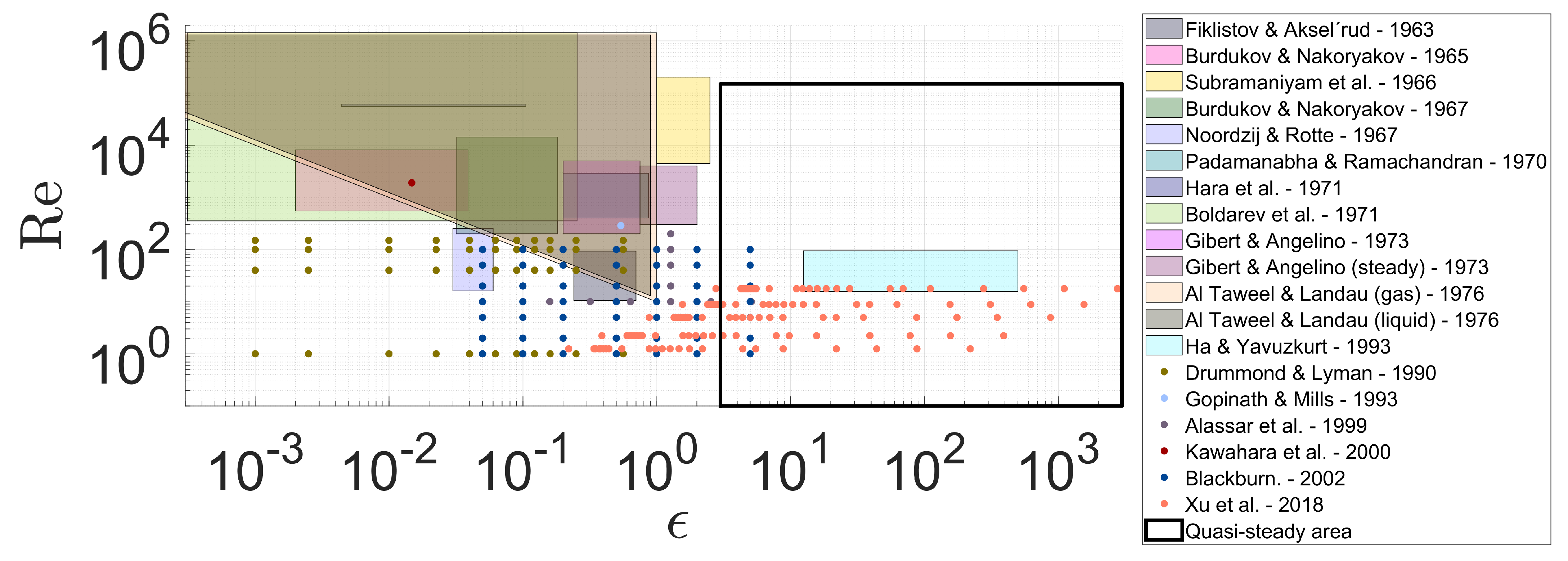
This threshold was suggested as by Gibert and Angelino [35] and supported by Al Taweel and Landau [29], while Drummond and Lyman [39] derived it to be . The general quasi-steady assumption for large is also supported by the theoretical work of Ha and Yavuzkurt [36] and the work of Subramaniyam et al. [29]. Additionally, the experimental work of Xu et al. [41] fit the quasi-steady assumption quite well, for but also . The simulation results of Blackburn [25] and Alassar et al. [40] match each other well and also match the steady-state assumption for . In light of the review of the bulk of recent data, the approach of modeling the HMT for large validly with the quasi-steady assumption is substantiated. Nevertheless, the exact quasi-steady limit remains unclear, but it is approximately . For the sake of a comprehensive approach and in order to avoid model discontinuities (which other authors accepted), is chosen as the quasi-steady limit in this work. Figure 2 shows all the available data, while colored patches indicate a correlation given by the respective authors and dots indicate single data points without a correlation provided. Additionally, a black rectangle marks the quasi-steady area, where a multitude of steady data is available. This quasi-steady area is handled first in the following Section 3.1.
3. Results
3.1. Steady HMT Models
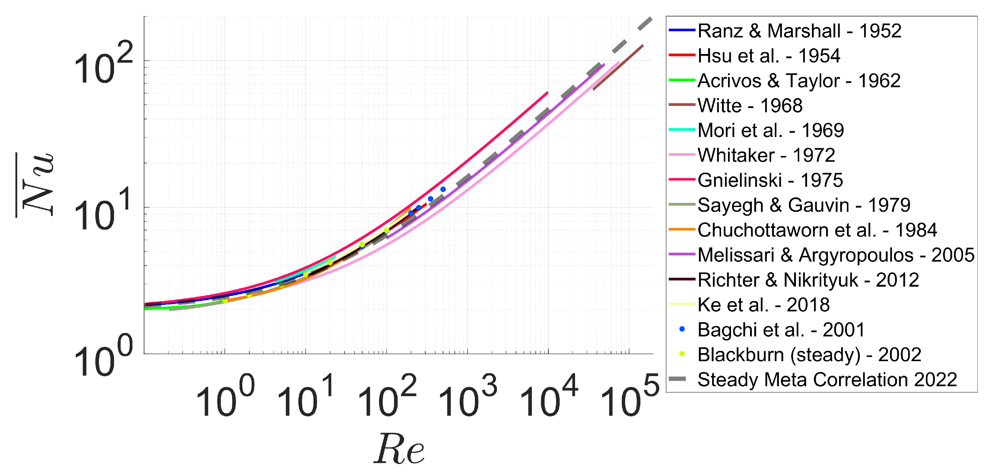
In accordance with the explanations in the previous section, the HMT for is modeled under the quasi-steady assumption. Therefore, a structured review of steady models for the HMT to particles was conducted. While meta-studies on this topic by Whitaker [16] and Gnielinski [17] provide good insights and also correlate a large number of works, they arrive at somewhat different correlations. So these two studies, along with central preceding studies, as well as newer experimental and numerical works are plotted in Figure 3. Solid lines indicate correlations given by the respective authors in the stated ranges of validity, or implicitly by the investigated ranges, while dots represent data points without a correlation provided by the authors. The dependencies of the investigated correlations on the Prandtl number (Schmidt number) are not considered in this work in order to achieve a better comparison of the Reynolds number dependencies. A meta-correlation of the steady Nusselt number (Sherwood number) averaged over the surface of the particle
is suggested for its simplicity, while fitting the data well. The normalized root-mean-square deviation () of each correlation or data set from the steady meta-correlation is provided in Table 1. The is calculated via
with the value of the respective correlation or single data point , the value of the meta-correlation , the value range of the respective correlation , and the number of sample points n. Note that the R2 value (coefficient of determination) is not a good measure for the correlation of nonlinear regressions [42] and is therefore not used here.
The meta-correlation fits most of the correlations very well with each . The only outlier is Witte (26.2%), which represents a special case with the investigation of the HMT from a tantalum sphere in liquid sodium. Based on the deviation from the other experimental setups and investigated systems, a somewhat different correlation is expected. Since the steady meta-correlation of this work over-predicts the lowest values of the meta-study by Whitaker (7.0%) to a similar degree as it under-predicts the highest values of the meta-study by Gnielinski (9.8%), it is deemed acceptable at this point based on the lack of any further data for spheres in high Reynolds number flows. Meta-Correlation (2) is now used in order to model the HMT to particles in oscillating flows for , together with the data from oscillating flows.
3.2. HMT Models for Oscillating Flows
Several works exist in the literature which have investigated the HMT to spheres in an oscillating flow with an . Their data fit the quasi-steady assumption often well or they suggested a steady correlation themselves, as discussed in Section 3.1. This is not the case for , where the amplitude parameter has to be taken into account, especially if, in addition to a small , also large Womersley numbers occur. In these cases, the streaming Reynolds number is significant, leading to an increased influence of steady streaming in the HMT process [7]. Most investigated authors account for the influence of steady streaming by correcting the steady HMT correlations with a term ‘’, or sometimes directly working with the streaming Reynolds number. Taxonomy (1) was updated to incorporate these models accordingly. The meta-study by Al Taweel and Landau [29], confined to the mass transfer due to steady streaming, laid the groundwork for this updated meta-study. On the one hand, unfortunately, some of their referenced papers are no longer available, leaving only the data as stated by Al Taweel and Landau. On the other hand, even more data could be retrieved from some of the works investigated by Al Taweel and Landau with the help of the relations presented in Figure A1. A detailed explanation of the conducted data preparation can be found in Appendix A. However, much more data from various recent works are available now, especially for a gaseous environment: Gopinath and Mills [38] based their work on the flow formulations by Riley [43] for the region of impactful steady streaming with and . They derived the governing equation of energy for this case, which is numerically solved along with the equation of motion in order to provide several data points for a regression. A simple experiment was conducted for the validation of the resulting correlation. Kawahara et al. [37] investigated the mass transfer from a camphor-covered sphere placed in a USL. They found good agreement with the experiments of Gopinath and Mills and Burdukov and Nakoryakov. Drummond and Lyman [39] applied a pseudospectral method in order to solve the NSEs and mass transport equations. They found a decreasing HMT for an increasing amplitude parameter, which is a unique result within the literature. Additionally, they suggested a quasi-steady limit of . Alassar et al. [40] solved the NSEs and energy equations for a Boussinesq fluid. The Prandtl number was assumed constant, , as was done in this work. While the authors investigated the forced and mixed convection regimes, only data for forced convection were utilized in this work for better comparability. Ha and Yavukurt [36] solved the two-dimensional, unsteady, laminar conservation equations for mass, momentum, and energy transport numerically in order to investigate the heat transfer to a particle. They found that for it can be approximated well with the steady HMT approach. Xu et al. [41] investigated the heat transfer from a coal particle in a power plant boiler in the presence of an acoustic field. The mathematical framework of Ha and Yavukurt was utilized, while the particle size was kept constant at 100 and the flue gas properties were kept constant at a temperature of 1200 . The oscillation frequency and oscillation amplitude were varied and they found a decrease in heat transfer intensity at , an increase at , and a decreasing dependency on the amplitude parameter for . The numerical calculations were validated by experiments with copper spheres in an acoustic field. Blackburn [25] investigated the heat and mass transfer to a particle in an oscillating flow numerically. The author also utilized the two defining dimensionless numbers of amplitude parameter and oscillating Reynolds number . Additionally, the steady case was calculated for comparison. Blackburn found a slightly decreased HMT intensity for the oscillating case compared with the steady case. Even though the author’s values for the steady case are slightly higher than in many other works, this is a unique result.
The HMT in gases and liquids are quite similar to each other since it is subject to the same physical phenomena and therefore often modeled similarly. Although the Prandtl numbers (Schmidt numbers) are commonly several magnitudes greater in gases than in liquids, the basic models and correlations are the same. In fact, the statements in this work so far can be applied to gases and liquids alike. This is not the case for steady streaming, where different asymptotic behavior could be observed for gases and liquids, necessitating a distinction of cases [29]. Therefore, similar to the approach for the steady models in the previous section, two meta-correlations were found covering the entire plane, each of which being applicable to either a gaseous or liquid environment, respectively. The Nusselt number (Sherwood number) is averaged over the particle surface and averaged over one oscillation cycle in this case:
4. Discussion
4.1. Meta-Correlation Design
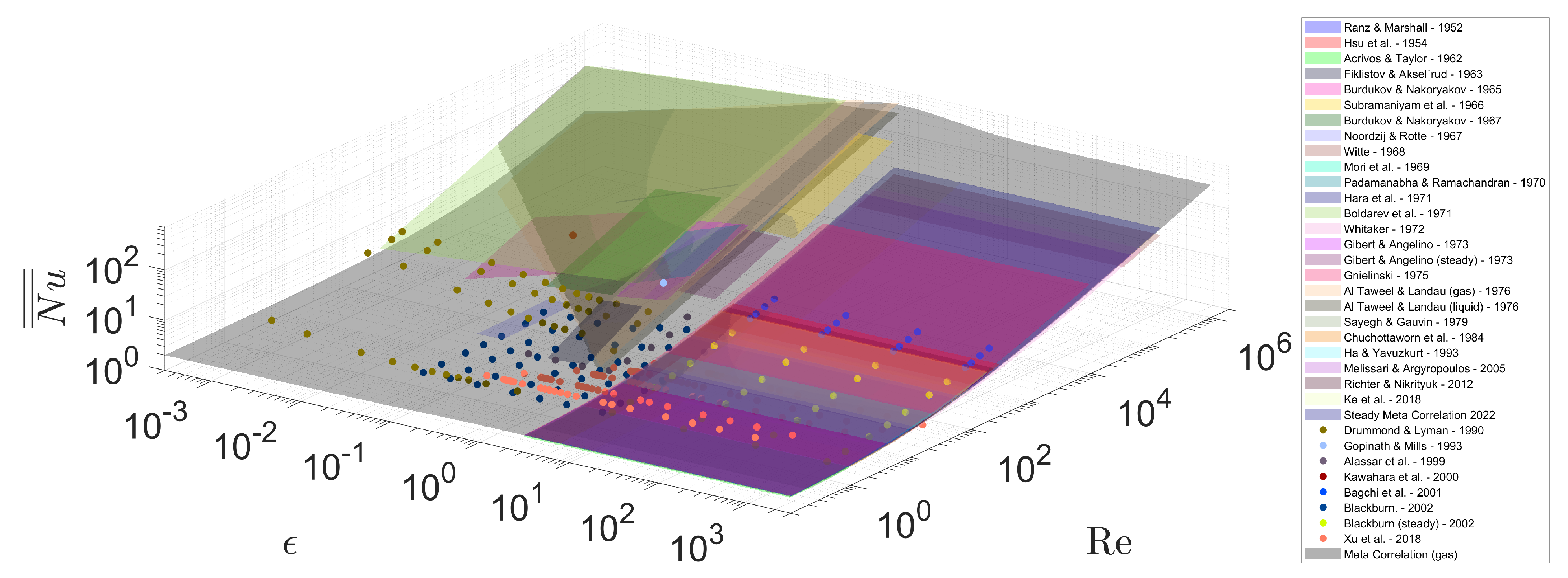
The plane captures the extremes of very small and very large amplitude parameters and Reynolds numbers. It was ensured that Meta-Correlations (4) and (5) follow all the various asymptotic behaviors that the experimental and theoretical works in the literature derived. For small Reynolds numbers, the conductive (diffusive) limit of for a sphere is ensured with term ‘A’. The quasi-steady behavior of is modeled with term ‘B’, which reflects the Steady Meta-Correlation (2). While term ‘C’ tends towards unity for large , term ’D’ tends towards zero. The steady Term ‘B’ is then corrected for with Term ‘C’. This term brings the dependency on and corrects the factor accordingly. Here, a distinction needs to be drawn between the asymptotic behavior in gases and liquids, hence the two correlations differ here. The enhancement of the HMT at , which is suggested by several models, is described by term ‘D’. By form, the standard normal distribution of a probability density function was utilized here. It describes the enhancement of the HMT at well, especially for . The expectation and the standard deviation were fitted well to values of zero and unity, respectively. This term also differs for gases and liquids, mostly in order to offset the difference in Term ‘C’ and to ensure model consistency. The split of correlations in the steady streaming area for gases and liquids in Figure 4 is noticeable, especially with their different asymptotic behavior for , while the asymptotic behavior for gases is captured well with Meta-Correlation (4).
4.2. Deviations
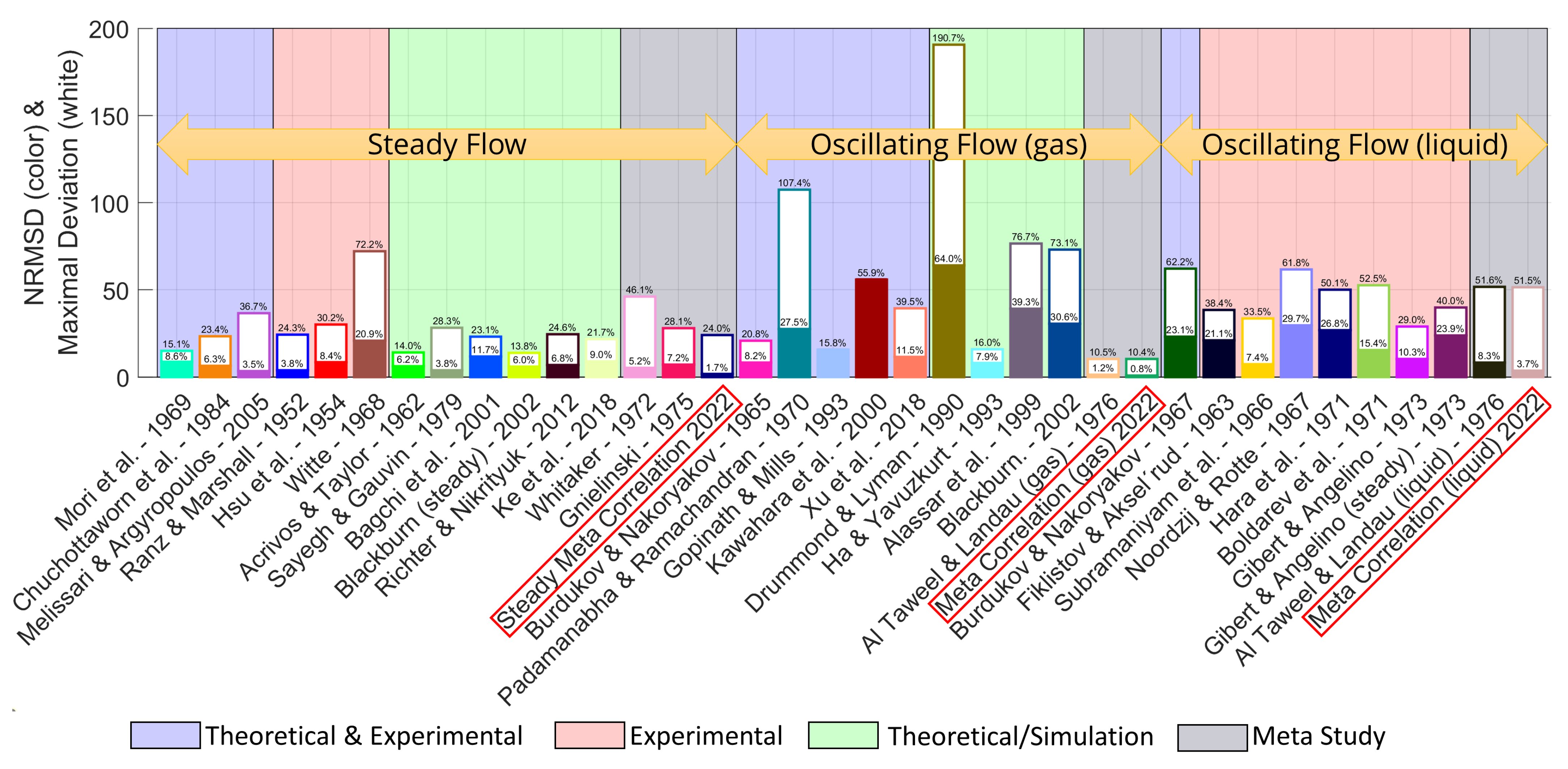
Figure 5 shows the deviations of Meta-Correlations (4) and (5) from the respective individual models.
The colored bars give the , calculated with Equation (3), while the white bars give the maximum normalized deviation. Meta-Correlations (4) and (5) deviate insignificantly from Steady Meta-Correlation (2) and from the investigated steady models in general, as pointed out in Section 3.1. While the correlations for steady flow behave very similarly, this is not so clear for oscillating flows. Besides the mentioned necessity for a distinction between gaseous and liquid flows, due to their different asymptotic behavior, the overall measured and simulated data diverge substantially. Drummond and Lyman are the obvious outlier here since they are the only authors who predicted an increase of HMT intensity with a decreasing amplitude parameter , which is also reflected in a large deviation of their data. Blackburn [25] commented on this study and suggested that the mesh resolution near the surface of the sphere might be too low. This would result in the inability to capture the flow behavior for small oscillation amplitudes properly. The other models for oscillating flow, which often cover the same region of the plane, deliver scattered data. This implies an insufficient experimental or simulation design by many authors, or additional dependencies beyond solely the oscillation Reynolds number and the amplitude parameter, contrary to the consensus in the literature. Nevertheless, based on the currently available data, Meta-Correlations (4) and (5) are viable, especially with regard to the large parameter ranges covering several orders. This is also reflected in their from all combined data of 0.8% for gases and 3.7% for liquids. Additionally, Meta-Correlations (4) and (5) only slightly deviate from the previous meta-analyses in their respective part of the plane (1.2% for gases and 8.3% for liquids).
4.3. Quasi-Steady Assumption
Often in the literature, the quasi-steady assumption is applied for the HMT to particles in oscillating flows. Figure 6 shows a comparison of Meta-Correlation (4) with the derived Steady Correlation (2). It shows that the quasi-steady approach is only valid for or . For , it under-predicts the intensity of the HMT, while it over-predicts the intensity of the HMT for and .
5. Conclusions
- the high number of 33 correlated data sets;
- the large size of the covered parameter space of amplitude parameter and Reynolds number and the comprehensive nature of the correlations;
- the carefully modeled asymptotic behavior for extreme values as the relevant literature suggests by theoretical considerations and a multitude of experiments;
- them highlighting the substantiated characteristics of a decreased HMT in the steady streaming region, an increased HMT for , and the quasi-steady HMT for .
The presented meta-correlations enable a direct prediction of the heat (and mass) transfer to a single, solid particle in an oscillating gas or liquid flow, with a known oscillating Reynolds number , amplitude parameter , and Prandtl number (or Schmidt number ).
Author Contributions
Conceptualization, methodology, writing—original draft preparation, writing—review and editing, and visualization, S.H.; supervision, project administration and funding acquisition, S.U. and M.B. All authors have read and agreed to the published version of the manuscript.
Funding
The authors would like to thank the Boysen-TU Dresden-Research Training Group for the financial support that has made this publication possible. The Research Training Group is co-financed by TU Dresden and the Friedrich and Elisabeth Boysen Foundation. Grant number: BOY-135.
Data Availability Statement
Data are available from the corresponding author upon reasonable request.
Acknowledgments
This publication is part of the dissertation of S. Heidinger, which is soon to be published as a comprehensive treatise on this topic.
Conflicts of Interest
The authors declare no conflict of interest.
Nomenclature
| A | displacement amplitude |
| m | mass |
| d | particle diameter |
| n | number of sample point |
| y | sample point |
| oscillation Reynolds number | |
| oscillation Stokes number | |
| Nusselt number | |
| Sherwood number | |
| Streaming Reynolds number | |
| U | slip velocity amplitude |
| Womersley number | |
| Prandtl number | |
| Schmidt number | |
| density ratio | |
| amplitude parameter | |
| boundary layer thickness | |
| difference | |
| dynamic viscosity | |
| density | |
| angular frequency |
Abbreviations
| heat and mass transfer | |
| normalized root mean square deviation | |
| standard temperature and pressure |
Indices
| p | particle |
| f | fluid |
Appendix A. Conducted Data Preparation
The paper by Al Taweel and Landau [29] was the source for some of the works listed in Table A1. The handling of these works was conducted as follows: there was an attempt to retrieve the original paper. If this was not possible, the information stated by Al Taweel and Landau was used. In this case, their paper was indicated as the source of the data. In case the original paper was available, the data were compared with Al Taweel and Landau. In some cases, they did not specify a value or range of a parameter, even though it could be indirectly retrieved by the relations in Figure A1 or by other relations in general. These steps in data preparation are listed here for each individual case:
- †
- Al Taweel and Landau did not provide a value range for the displacement amplitude A and stated only that the amplitude parameter is much smaller than unity for the work of Burdukov and Nakoryakov [28]. While this statement agrees with the respective paper, also the applied decibel range of the utilized levitator is stated in that paper: 150 dB to 163 dB. With the standard reference sound pressure level of [44] and the linear relation between pressure amplitude P and velocity amplitude , , with the speed of sound c in the fluid, the fluid velocity amplitude was calculated. Since no significant particle relaxation occurs [10], the slip velocity amplitude was set equal to the fluid velocity amplitude as given in Table A1. Subsequently, the displacement amplitude and the amplitude parameter were calculated according to the relations in Figure A1.
- ‡
- Al Taweel and Landau did not provide a value for the spheres’ diameter, but in the original paper of Burdukov and Nakoryakov [31] is stated that the glass spheres with mount weighed about . Additionally, the thickness of benzoic acid coating was about 0.6 to 1 , with a weight of about . This information opens up two ways of estimating the diameter of the glass sphere:
- Neglecting the weight of the mount and assuming the utilization of borosilicate glass, which is often used in a scientific environment, with a density of about [45], the diameter can be calculated to aboutIn case ordinary glass (soda–lime) was used with a density of , the spheres would be insignificantly smaller.
- Calculating the dimensions of the coating by assuming a benzoic acid density of [46], the diameter can be calculatedEven though Equation (A4) has two theoretical solutions due to its quadratic nature, only the physically plausible solution with a positive diameter was chosen.In approaches 1 and 2, the diameter of the spheres can be estimated to be . Therefore, this value is used in this work. Still, this problem is undetermined and the determination of another parameter is necessary in order to calculate all the parameters listed in Table A1. In the original paper is stated that the frequency varied from 10 to 125 translating to angular frequencies of 63 s−1 to 785 s−1. All other input properties listed in the first row of Figure A1 are kept constant except the velocity amplitude U, which is dependent on the frequency. The parameter in the original paper was varied between 100 and 1200. The Schmidt number was estimated by Al Taweel and Landau to be approximately 1000 in this setup. Adopting this value and linking low oscillation frequencies to low-velocity amplitudes and high oscillation frequencies to high-velocity amplitudes delivers an investigated velocity amplitude window of approximately 0.02 m s−1 to 1.43 m s−1. With these values, all the parameters listed in Table A1 can be determined via the relations in Figure A1.
- One parameter is missing in the original paper [34] in order to calculate all the values listed in Table A1. The velocity amplitude is calculated via the same approach as in the previous paragraph. The parameter is varied between 25 and 100 in the original paper while keeping all parameters except the oscillation frequency constant. This translates with to a velocity amplitude window of about 0.24 m s−1 to 239 m s−1.
Table A1.
A list of investigated works by Al Taweel and Landau [29]. Some of their stated data have been marked () and expanded with information from the original papers.
Table A1.
A list of investigated works by Al Taweel and Landau [29]. Some of their stated data have been marked () and expanded with information from the original papers.
| Authors | [s] | (m) | (m) | (m s) | (m s) | ( - ) | ( - ) | Source |
| Fiklistov and Aksel’rud | 3.8 33.3 | 1.2 × 10⁻³ 3.5 × 10⁻³ | 5× 10⁻³ | 2.1× 10⁻³ 1.9× 10⁻² | 10−6 | 0.24 0.7 | 10.5 93.5 | [27] |
| Burdukov and Nakoryakov † | 7.2 × 10⁴ 1.1 × 10⁵ | 2.0 × 10⁻⁵ 1.4 × 10⁻⁴ | 3.5 × 10⁻³ 10−2 | 2.2 9.8 | 1.2 × 10⁻⁵ | 2 × 10⁻³ 4.5 × 10⁻² | 5.5 × 10² 8.4 × 10³ | [28] |
| Subramaniyam et al. | 25 126 | 2.7 × 10⁻² 3.7 × 10⁻² | 1.3 × 10⁻² 2.5 × 10⁻² | 0.3 8.0 | 10−6 | 1 2.5 | 4.5 × 10³ 2.0 × 10⁵ | [29] [30] |
| Burdukov and Nakoryakov ‡ | 63 785 | 3.2 × 10⁻⁴ 1.8 × 10⁻³ | 1 × 10⁻² | 2 × 10⁻² 1.4 | 10−6 | 3.2 × 10⁻² 0.18 | 2 × 10² 1.4 × 10⁴ | [31] |
| Noordzij and Rotte | 0 220 | 7.8 × 10⁻⁴ 1.6 × 10⁻³ | 2.5 × 10⁻² | 0.17 0.33 | 10−6 | 3 × 10⁻² 6 × 10⁻² | 16 2.6 × 10² | [29] [32] |
| Padamanabha and Ramachandran | 19 63 | 1 × 10⁻² 2.2 × 10⁻² | 2.5 × 10⁻² 5 × 10⁻² | 0.19 1.38 | 1.2 × 10⁻⁵ | 0.2 0.87 | 4 × 10² 2.9 × 10³ | [33] |
| Hara et al. | 1.2 × 10⁴ 1.2 × 10⁵ | 4.4 × 10⁻⁵ 7.2 × 10⁻⁴ | 6.8 × 10⁻³ 10−2 | 5.5 9.0 | 10−6 | 4.4 × 10⁻³ 0.11 | 5.5 × 10⁴ 6.1 × 10⁴ | [29] |
| Boldarev et al. | 1.3 × 10⁵ 6.3 × 10⁶ | 1.9 × 10⁻⁶ 3.8 × 10⁻⁵ | 1.5 × 10⁻⁴ 6 × 10⁻³ | 0.24 239 | 10−6 | 3.1 × 10⁻⁴ 0.25 | 35.4 1.4 × 10⁶ | [34] |
| Gibert and Angelino | 5 25 | 1.6 × 10⁻³ 2.3 × 10⁻² | 8 × 10⁻³ 3 × 10⁻² | 6.6 × 10⁻³ 6.3 × 10⁻¹ | 10−6 | 0.2 0.75 | 2 × 10² 5 × 10³ | [35] |
| Gibert and Angelino | 5 25 | 6 × 10⁻³ 6.1 × 10⁻² | 8 × 10⁻³ 3 × 10⁻² | 9.8 × 10⁻³ 0.5 | 10−6 | 0.75 2 | 3 × 10² 4 × 10³ | [35] |
Appendix B. Central Dimensionless Numbers in Oscillating Flows
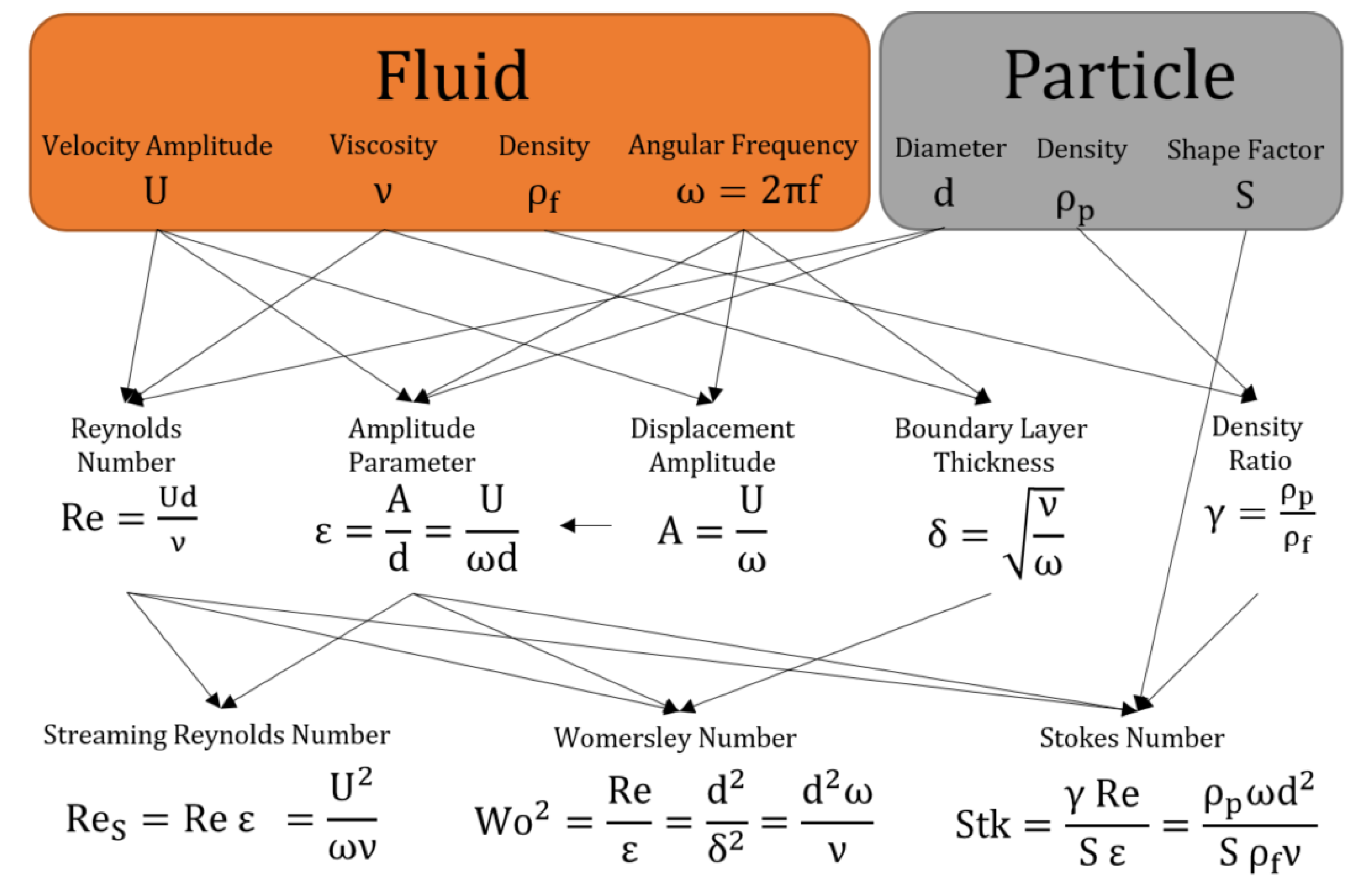
Figure A1.
Derivation and relations of central dimensionless numbers.

References
- Rothlisberger, M.; Schmidli, G.; Schuck, M.; Kolar, J.W. Multi-Frequency Acoustic Levitation and Trapping of Particles in All Degrees of Freedom. IEEE Trans. Ultrason. Ferroelectr. Freq. Control 2022, 69, 1572–1575. [Google Scholar] [CrossRef] [PubMed]
- Wang, Y.; Wu, L.; Wang, Y. Study on Particle Manipulation in a Metal Internal Channel under Acoustic Levitation. Micromachines 2021, 13, 18. [Google Scholar] [CrossRef] [PubMed]
- Heidinger, S.; Spranger, F.; Dostál, J.; Zhang, C.; Klaus, C. Material Treatment in the Pulsation Reactor—From Flame Spray Pyrolysis to Industrial Scale. Sustainability 2022, 14, 3232. [Google Scholar] [CrossRef]
- Klaus, C.; Wegner, K.; Rammelt, T.; Ommer, M. New Challenges in Thermal Processing. Interceram—Int. Ceram. Rev. 2021, 70, 22–25. [Google Scholar] [CrossRef]
- Hoffmann, C.; Ommer, M. Reaktoren für Fluid-Feststoff-Reaktionen: Pulsationsreaktoren. In Handbuch Chemische Reaktoren; Reschetilowski, W., Ed.; Springer Reference Naturwissenschaften; Springer: Berlin/Heidelberg, Germany, 2019; pp. 1–19. [Google Scholar] [CrossRef]
- Womersley, J.R. Method for the calculation of velocity, rate of flow and viscous drag in arteries when the pressure gradient is known. J. Physiol. 1955, 127, 553–563. [Google Scholar] [CrossRef]
- Riley, N. Steady Streaming. Annu. Rev. Fluid Mech. 2001, 33, 43–65. [Google Scholar] [CrossRef]
- Wang, C.Y. On high-frequency oscillatory viscous flows. J. Fluid Mech. 1968, 32, 55–68. [Google Scholar] [CrossRef]
- Chong, K.; Kelly, S.D.; Smith, S.; Eldredge, J.D. Inertial particle trapping in viscous streaming. Phys. Fluids 2013, 25, 033602. [Google Scholar] [CrossRef] [Green Version]
- Heidinger, S.; Unz, S.; Beckmann, M. Simple Particle Relaxation Modeling in One-Dimensional Oscillating Flows. Processes 2022, 10, 1322. [Google Scholar] [CrossRef]
- Valverde, J.M. Acoustic streaming in gas-fluidized beds of small particles. Soft Matter 2013, 9, 8792. [Google Scholar] [CrossRef]
- Yavuzkurt, S.; Ha, M.Y. A Model of the Enhancement of Combustion of Coal-Water Slurry Fuels Using High-Intensity Acoustic Fields. J. Energy Resour. Technol. 1991, 113, 268–276. [Google Scholar] [CrossRef]
- Mori, Y.; Imabayashi, M.; Hijikata, K.; Yoshida, Y. Unsteady heat and mass transfer from spheres. Int. J. Heat Mass Transf. 1969, 12, 571–585. [Google Scholar] [CrossRef]
- Ranz, W.E.; Marshall, W.R. Vaporation from drops, Part I. Chem. Eng. Progr. 1952, 48, 141–146. [Google Scholar]
- Hsu, N.T.; Sato, K.; Sage, B.H. Material Transfer in Turbulent Gas Streams. Ind. Eng. Chem. 1954, 46, 870–876. [Google Scholar] [CrossRef]
- Whitaker, S. Forced convection heat transfer correlations for flow in pipes, past flat plates, single cylinders, single spheres, and for flow in packed beds and tube bundles. AIChE J. 1972, 18, 361–371. [Google Scholar] [CrossRef]
- Gnielinski, V. Berechnung mittlerer Wärme- und Stoffübergangskoeffizienten an laminar und turbulent überströmten Einzelkörpern mit Hilfe einer einheitlichen Gleichung. Forsch. Ingenieurwesen 1975, 41, 145–153. [Google Scholar] [CrossRef]
- Ke, C.; Shu, S.; Zhang, H.; Yuan, H.; Yang, D. On the drag coefficient and averaged Nusselt number of an ellipsoidal particle in a fluid. Powder Technol. 2018, 325, 134–144. [Google Scholar] [CrossRef]
- Richter, A.; Nikrityuk, P.A. Drag forces and heat transfer coefficients for spherical, cuboidal and ellipsoidal particles in cross flow at sub-critical Reynolds numbers. Int. J. Heat Mass Transfer 2012, 55, 1343–1354. [Google Scholar] [CrossRef]
- Sayegh, N.N.; Gauvin, W.H. Numerical analysis of variable property heat transfer to a single sphere in high temperature surroundings. AIChE J. 1979, 25, 522–534. [Google Scholar] [CrossRef]
- Melissari, B.; Argyropoulos, S.A. Development of a heat transfer dimensionless correlation for spheres immersed in a wide range of Prandtl number fluids. Int. J. Heat Mass Transf. 2005, 48, 4333–4341. [Google Scholar] [CrossRef]
- Witte, L.C. An Experimental Study of Forced-Convection Heat Transfer From a Sphere to Liquid Sodium. J. Heat Transf. 1968, 90, 9–12. [Google Scholar] [CrossRef]
- Chuchottaworn, P.; Fujinami, A.; Asano, K. Experimental study of evaporation of a volatile pendant drop under high mass flux conditions. J. Chem. Eng. Jpn. 1984, 17, 7–13. [Google Scholar] [CrossRef] [Green Version]
- Bagchi, P.; Ha, M.Y.; Balachandar, S. Direct Numerical Simulation of Flow and Heat Transfer From a Sphere in a Uniform Cross-Flow. J. Fluids Eng. 2001, 123, 347–358. [Google Scholar] [CrossRef]
- Blackburn, H.M. Mass and momentum transport from a sphere in steady and oscillatory flows. Phys. Fluids 2002, 14, 3997–4011. [Google Scholar] [CrossRef]
- Acrivos, A.; Taylor, T.D. Heat and Mass Transfer from Single Spheres in Stokes Flow. Phys. Fluids 1962, 5, 387. [Google Scholar] [CrossRef]
- Fiklistov, I.N.; Aksel’rud, G.A. Kinetics of mass transfer between a bed of solid particles and a pulsating stream of liquid. J. Eng. Phys. 1963, 10, 312–316. [Google Scholar] [CrossRef]
- Burdukov, A.P.; Nakoryakov, V.E. On mass transfer in an acoustic field. J. Appl. Mech. Tech. Phys. 1965, 6, 51–55. [Google Scholar] [CrossRef]
- Al Taweel, A.M.; Ismail, M.I. Comparative analysis of mass transfer at vibrating electrodes. J. Appl. Electrochem. 1976, 6, 559–564. [Google Scholar] [CrossRef]
- Al Taweel, A.M.; Landau, J. Mass transfer between solid spheres and oscillating fluids—A critical review. Can. J. Chem. Eng. 1976, 54, 532–539. [Google Scholar] [CrossRef]
- Burdukov, A.P.; Nakoryakov, V.E. Effects of vibrations on mass transfer from a sphere at high prandtl numbers. J. Appl. Mech. Tech. Phys. 1967, 8, 111–113. [Google Scholar] [CrossRef]
- Noordzij, M.P.; Rotte, J.W. Mass-transfer coefficients for a simultaneously rotating and translating sphere. Chem. Eng. Sci. 1967, 23, 657–660. [Google Scholar] [CrossRef]
- Padamanabha, D.; Nair, B.G.; Ramachandran, A. Effect of vertical vibration on mass transfer from spheres. Indian J. Technol. 1970, 8, 243–247. [Google Scholar]
- Boldarev, A.M.; Burdukov, A.P.; Nakoryakov, V.E.; Sosunov, V.I. Investigation of the effect of ultrasonic vibrations on mass transfer from a sphere, with large prandtl numbers. J. Appl. Mech. Tech. Phys. 1971, 12, 295–297. [Google Scholar] [CrossRef]
- Gibert, H.; Angelino, H. Influence de la pulsation sur les transferts de matière entre une sphère et un liquide. Can. J. Chem. Eng. 1973, 51, 319–325. [Google Scholar] [CrossRef]
- Ha, M.Y.; Yavuzkurt, S.; Kim, K.C. Heat transfer past particles entrained in an oscillating flow with and without a steady velocity. Int. J. Heat Mass Transf. 1993, 36, 949–959. [Google Scholar] [CrossRef]
- Kawahara, N.; Yarin, A.L.; Brenn, G.; Kastner, O.; Durst, F. Effect of acoustic streaming on the mass transfer from a sublimating sphere. Phys. Fluids 2000, 12, 912–923. [Google Scholar] [CrossRef]
- Gopinath, A.; Mills, A.F. Convective Heat Transfer From a Sphere Due to Acoustic Streaming. J. Heat Transf. 1993, 115, 332–341. [Google Scholar] [CrossRef]
- Drummond, C.K.; Lyman, F.A. Mass transfer from a sphere in an oscillating flow with zero mean velocity. Comput. Mech. 1990, 6, 315–326. [Google Scholar] [CrossRef] [Green Version]
- Alassar, R.S.; Badr, H.M.; Mavromatis, H.A. Heat convection from a sphere placed in an oscillating free stream. Int. J. Heat Mass Transf. 1999, 42, 1289–1304. [Google Scholar] [CrossRef]
- Xu, W.; Jiang, G.; An, L.; Liu, Y. Numerical and experimental study of acoustically enhanced heat transfer from a single particle in flue gas. Combust. Sci. Technol. 2018, 190, 1158–1177. [Google Scholar] [CrossRef]
- Spiess, A.N.; Neumeyer, N. An evaluation of R2 as an inadequate measure for nonlinear models in pharmacological and biochemical research: A Monte Carlo approach. BMC Pharmacol. 2010, 10, 6. [Google Scholar] [CrossRef] [PubMed]
- Riley, N. On a Sphere Oscillating in a Viscous Fluid. Q. J. Mech. Appl. Math. 1966, 19, 461–472. [Google Scholar] [CrossRef]
- IEC 61672-1:2013; Electroacoustics—Sound Level Meters. International Electrotechnical Commission: Geneva, Switzerland, 2013.
- Bansal, N.P.; Doremus, R.H. Handbook of Glass Properties; Academic Press Handbook Series; Academic Press: Orlando, FL, USA, 1986. [Google Scholar]
- Zakel, S.; Brandes, E.; Schröder, V. Reliable safety characteristics of flammable gases and liquids—The database CHEMSAFE. J. Loss Prev. Process. Ind. 2019, 62, 103914. [Google Scholar] [CrossRef]
Figure 1.
- plane by Heidinger et al. [10] in which all flow states of a single particle in an oscillating flow can be defined. Note that the origin has the coordinates .
Figure 1.
- plane by Heidinger et al. [10] in which all flow states of a single particle in an oscillating flow can be defined. Note that the origin has the coordinates .

Figure 2.
Overview of considered experimental and numerical data and correlations for the HMT to particles in oscillating flows. Colored patches indicate a provided correlation by the authors, while single points indicate individual measurement or simulation points without a correlation provided by the respective authors. All the sources of the data are listed in Table 1.

Figure 3.
Overview of considered experimental and numerical HMT data for single spherical particles in steady flow. Solid lines indicate correlations provided by the respective authors, while single points indicate individual measurements or simulation points without correlations provided by the authors. Additionally, Steady Meta-Correlation (2) is plotted, which is fitted to the listed data. The Prandtl number is set to as it can be found with air at STP. All the sources of the data are listed in Table 1.

Figure 4.
Nusselt number averaged over the particle surface and averaged over one oscillation cycle predicted by various investigated models plotted in the - plane. Additionally, Meta-Correlation (4) for gaseous environments is plotted, while the Prandtl number is set to as can be found with air at STP.

Figure 5.
Deviations of Meta-Correlation (4) and (5) to the respective individual models investigated and listed in Table 1. The colored bars give the , calculated with Equation (3), while the white bars give the maximum normalized deviation. The deviation presented for Meta-Correlations (4) and (5) is for all investigated models and data combined.


Disclaimer/Publisher’s Note: The statements, opinions and data contained in all publications are solely those of the individual author(s) and contributor(s) and not of MDPI and/or the editor(s). MDPI and/or the editor(s) disclaim responsibility for any injury to people or property resulting from any ideas, methods, instructions or products referred to in the content. |
© 2023 by the authors. Licensee MDPI, Basel, Switzerland. This article is an open access article distributed under the terms and conditions of the Creative Commons Attribution (CC BY) license (https://creativecommons.org/licenses/by/4.0/).
Share and Cite
MDPI and ACS Style
Heidinger, S.; Unz, S.; Beckmann, M. Heat and Mass Transfer to Particles in One-Dimensional Oscillating Flows. Processes 2023, 11, 173. https://doi.org/10.3390/pr11010173
AMA Style
Heidinger S, Unz S, Beckmann M. Heat and Mass Transfer to Particles in One-Dimensional Oscillating Flows. Processes. 2023; 11(1):173. https://doi.org/10.3390/pr11010173
Chicago/Turabian StyleHeidinger, Stefan, Simon Unz, and Michael Beckmann. 2023. "Heat and Mass Transfer to Particles in One-Dimensional Oscillating Flows" Processes 11, no. 1: 173. https://doi.org/10.3390/pr11010173
Note that from the first issue of 2016, this journal uses article numbers instead of page numbers. See further details here.