

Performance of a Novel Enhanced Sparrow Search Algorithm for Engineering Design Process: Coverage Optimization in Wireless Sensor Network

1
College of Electronic Information, Guangxi Minzu University, Nanning 530006, China
2
Guangxi Key Laboratory of Hybrid Computation and IC Design Analysis, Guangxi Minzu University, Nanning 530006, China
3
School of Artificial Intelligence, Guangxi Minzu University, Nanning 530006, China
*
Author to whom correspondence should be addressed.
Processes 2022, 10(9), 1691; https://doi.org/10.3390/pr10091691
Submission received: 26 July 2022
/
Revised: 18 August 2022
/
Accepted: 22 August 2022
/
Published: 25 August 2022
(This article belongs to the Special Issue Evolutionary Process for Engineering Optimization (II))
Abstract
:Burgeoning swarm intelligence techniques have been creating a feasible theoretical computational method for the modeling, simulation, and optimization of complex systems. This study aims to increase the coverage of a wireless sensor network (WSN) and puts forward an enhanced version of the sparrow search algorithm (SSA) as a processing tool to achieve this optimization. The enhancement of the algorithm covers three aspects. Firstly, the Latin hypercube sampling technique is utilized to generate the initial population to obtain a more uniform distribution in the search space. Secondly, a sine cosine algorithm with adaptive adjustment and the Lévy flight strategy are introduced as new optimization equations to enhance the convergence efficiency of the algorithm. Finally, to optimize the individuals with poor fitness in the population, a novel mutation disturbance mechanism is introduced at the end of each iteration. Through numerical tests of 13 benchmark functions, the experimental results show that the proposed enhanced algorithm can converge to the optimum faster and has a more stable average value, reflecting its advantages in convergence speed, robustness, and anti-local extremum ability. For the WSN coverage problem, this paper established a current optimization framework based on the swarm intelligence algorithms, and further investigated the performance of nine algorithms applied to the process. The simulation results indicate that the proposed method achieves the highest coverage rate of 97.66% (on average) among the nine algorithms in the calculation cases, which is increased by 13.00% compared with the original sparrow search algorithm and outperforms other methods by 1.47% to 15.34%.
1. Introduction
A wireless sensor network (WSN) is a practical intelligent information acquisition system composed of a certain number of sensor nodes with communication, computing, sensing, and other functions deployed in the area to be monitored. Owing to its advantages of economic applicability and fault tolerance, WSNs have been increasingly prevalent in agricultural management [1], intelligent medical services [2,3], advanced communication [4], and Internet of Things (IoT) [5,6]. By and large, the design of a WSN confronts many constraints and challenges, and the coverage optimization for monitoring areas is a fundamental issue that any type of WSNs need to solve [7]. In some scenarios, the application of a WSN is restricted by the actual physical conditions. Random deployment is the simplest method, but it often leads to uneven distribution, high overlap, and low coverage, which remarkably affects the quality of service for a WSN. Consequently, an intelligent nodes deployment method is necessary. As one direct means of implementation, the deployment optimization of sensor nodes is of great significance to improve the sensing performance and work efficiency of a WSN.
In recent years, metaheuristics have provided flexible solutions to various optimization problems. As an efficient branch, swarm intelligence has the characteristics of coevolution and more robust population optimization [8,9], which has attracted the attention of many scholars and has made some progress in the application study of WSN coverage optimization. Liao W et al. (2011) [10] and Yoon Y et al. (2013) [11], respectively, proposed sensor nodes deployment schemes based on the ant colony optimization algorithm and genetic algorithm for the problem, which increased the coverage area of a WSN and extended its service life. Wang L et al. (2018) [12] used the reverse learning strategy to improve the whale optimization algorithm and applied it to a probability-aware WSN model to enhance its coverage. Wang X et al. (2018) [13] improved particle swarm optimization by using the resampling method based on particle swarm optimization to ensure the activity of the population to a certain extent and applied the optimized algorithm to the coverage control problem. Miao Z et al. (2020) [14] proposed an improved grey wolf optimizer that consolidated the leadership of α gray wolf, and the applicability of the algorithm has been confirmed in the solution of WSN coverage optimization. Zhu F et al. (2021) [15] proposed a node simulation optimization method based on the improved weed algorithm before the actual deployment of the network. By introducing the differential evolution strategy and the disturbance mechanism, the improved algorithm has a more efficient convergence speed and a deployment scheme that can guide manual or robot placement of nodes is obtained. Mohammad Shokouhifar (2021) [16] proposed a practical multi-objective optimization algorithm based on the combination of the whale optimization algorithm and simulated annealing. With the objective function of maximizing the network coverage and minimizing the total cost, it has been successfully applied to radio frequency identification (RFID) network planning in the hospital environment, greatly reducing the total cost of the RFID network and achieving the goal of tracking medical assets. He Q et al. (2022) [17] proposed a marine predator algorithm with dynamic inertia weight and a multi-elite learning mechanism, which has improved the WSN coverage rate compared with the original algorithm. However, the improved algorithm converges slowly in the early iterations, which leads to unstable coverage. In this problem, the coverage optimization algorithms based on swarm intelligence are capable of obtaining the deployment schemes of sensor nodes more conveniently through the black box operation mechanism. In these cases, the performance of the algorithm is a key factor affecting the deployment quality. Hence, it is also crucial to perfect the algorithm, which can considerably make a difference to the results of WSN coverage optimization.
In this context, by correcting the defects of the sparrow search algorithm [18], this paper introduces a WSN sensor nodes deployment optimization method based on the augmentation of SSA, and names the new algorithm as a novel enhanced SSA (NESSA). Firstly, NESSA uses Latin hypercube sampling (LHS) to initialize the population, which ensures that the initial variables can effectively cover the search space and facilitates the rationality of the initial population distribution compared with the original random initialization method. Secondly, from the perspective of improving the performance and applicability to specific optimization problems, the original version is enhanced by using a sine cosine algorithm iteration and Lévy flight strategy, respectively. The results obtained are validated by the experimental data feedback and have achieved good performance in the subsequent WSN coverage optimization. Finally, based on the warning disturbance mechanism of the original algorithm, NESSA introduces a disruption phase for the population with poor fitness. Its principle is to utilize the information of the optimal individual to guide the worse population, so as to improve their optimization quality. This measure enriches the diversity of the population and is conducive to boosting the convergence and efficiency of the algorithm. To sum up, the contributions of our paper are mainly reflected in the following three aspects:
- A novel enhanced SSA version is implemented from the perspective of applicability and utilized to maximize the WSN coverage rate.
- A swarm intelligence applicable optimization process for the WSN coverage enhancement problem is established.
- The performance of other well-known swarm intelligence algorithms in WSN coverage optimization is further investigated and analyzed.
The rest of the paper is organized in the following manner. In Section 2, we first discuss the iterative mechanism of SSA and clarify the motivation for the improvement in this study, then expound in detail on the mathematical model of NESSA based on the augmentation part, and finally use the benchmark functions to conduct a numerical comparison experiment on the enhanced version to verify the effectiveness of the improved strategy. In Section 3, we introduce the mathematical model of WSN coverage optimization and set up a universal optimization process based on the swarm intelligence algorithm. Then, we further investigate the coverage optimization performance of nine swarm intelligence algorithms for three cases under this framework. In Section 4, we summarize some conclusions of this paper and look forward to future research directions.
2. Mathematical Model of Optimization Algorithm
The beginning of this section discusses the standard SSA metaheuristics, describing its known drawbacks. The improvement strategies to overcome these shortcomings are provided in detail and a novel enhanced SSA metaheuristics is proposed. Finally, the performance of the new algorithm is validated by numerical experiments.
2.1. Overview of the Standard SSA Metaheuristics
The standard SSA metaheuristic is a swarm intelligence algorithm proposed by Jiankai Xue et al. (2020) [18]. Its motivation comes from the foraging behavior of the sparrow population and the biological characteristics of avoiding natural enemies. To make the algorithm work in the actual optimization, SSA idealizes the sparrow individuals through several approximation rules and divides the constructed mathematical model into the following four iterative stages.
2.1.1. Initialization of Sparrow Population
SSA initializes the population in the form of random distribution, and the sparrows used for searching can be expressed as , where represents the dimension of the optimization problem variable. Generally, when all sparrow individuals have the same boundary, the randomly initialized population is:
where X represents the sparrow population, represents a random number matrix of , and and represent the upper and lower boundaries of sparrows, respectively.
2.1.2. The Producer Update Phase
SSA stipulates that producers are sparrows with the highest fitness in the population, are the learning objects of other individuals, and play a role in providing an evolutionary direction for the whole population. The updated equation for the producer is as follows:
where is the current iteration, is the maximum iteration, is the random number on (0,1], is the random number subject to a Normal Distribution, and is the ones matrix of . and represent the alarm value and the safety threshold, respectively, which are used as the adjustment parameters of the producer. In this paper, is set as the random value, while is defined as a fixed value of 0.8, which is consistent with the reference [18].
2.1.3. The Scrounger Update Phase
SSA defines the part whose fitness ranks behind all producers as the scrounger. These sparrows follow producers to improve their locations in the search space and are a supplement to producers. Their identities are in dynamic balance with producers in each iteration. The updated equation for the scrounger is as follows:
where is the best location found by the producer, is the current worst location, is a matrix, its internal elements are 1 or −1, and , and are the same as Equation (2).
2.1.4. The Scouter Update Phase
After the iteration of producers and scroungers, SSA randomly selects a certain proportion of sparrows in the population as scouters and updates their locations in each iteration. The updated equation for the scouter is as follows:
where is the current global optimal location, and are the control parameters, is the individual fitness, and is a minimal constant to avoid the denominator being 0, which is set as , and , respectively, represent the current global optimal fitness and the worst fitness.
2.2. Motivation for Improvements
Although previous studies have indicated that SSA has made significant progress in some practical challenges in the engineering field [19,20], these successful applications are often established based on the improved algorithms [21,22,23,24]. Solving the defects faced by standard SSA and adopting more appropriate improvement strategies to supplement and replace the algorithm framework are crucial prerequisites for attaining better performance indicators in engineering problems. For the iterative framework of standard SSA, we have the following conclusions to expound.
For the initialization phase of SSA, mapping variables in the search space using the random method tends to cause a lack of population diversity and a reduction in the ability to resist local extremum, which harms the convergence speed and accuracy of the algorithm. Thus, improving the quality of the initial population is meaningful work. Moreover, SSA also faces the disadvantage that the convergence becomes slower in the later iteration. Through the analysis of Equation (2), it can be seen that the update of producers is only affected by the individuals of the previous generation and lacks the guidance of the global optimal solution. When , the value range of the population is gradually reduced by the influence of [25], forming a typical “narrow search mode” tending to zero. Although this strategy facilitates the development ability of the algorithm and enables it to deeply mine the current region, in solving some problems, it is more necessary to ensure the breadth of the search scope and to find a promising area in the search space. Consequently, the current strategy at this phase is not always applicable. In addition, enhancing the exploration ability of scroungers to boost the chances of turning them into producers can reduce the possibility of the algorithm falling into stagnation, and effectively disturb the individuals with lower fitness ranking, which is helpful with the algorithm to search for the global optimal solution of the problem more efficiently.
It is worth noting that, as the “no free lunch” theorem reveals [26], no learning algorithm can provide the best solution to all problems. Hence, based on extensive empirical simulation, this study considers the improvement of SSA from the application side of WSN coverage optimization and enables the designed new algorithm to attain positive feedback results in the simulation test of the benchmark functions.
2.3. Proposed Novel Enhanced SSA Metaheuristics
A novel enhanced SSA version proposed in this study addresses issues of the standard SSA by assimilating the following strategies:
- Uniform population initialization based on Latin hypercube sampling;
- The sine and cosine iteration equations for the producer update phase;
- The scrounger update phase with Lévy flight;
- The disruption phase acts on the worse population with poor fitness.
2.3.1. Latin Hypercube Sampling Initialization
Latin hypercube sampling (LHS) is a multidimensional stratified sampling technique proposed by McKay et al. (1979) [27], which has the advantage of obtaining tail sample values under fewer sampling conditions.
Assuming that the sample size is 30, the distribution of LHS and random method in [0, 1] under two-dimensional conditions is illustrated in Figure 1. It can be seen that the sample distribution generated by LHS is wider than the area covered by the random one, and it meets the randomness of sampling [28]. Thus, LHS can form more uniform points in the search space, improve the diversity of the population, and lay a solid foundation for the optimization of the algorithm.
The steps of initializing the sparrow population using the LHS strategy with uniform stratification and equal probability sampling are as follows:
- (1)
- The population , dimension , and the boundary of individual sparrows are set.
- (2)
- The of each individual is divided into three sub-intervals that do not overlap each other and have the same probability.
- (3)
- One point is randomly selected from each sub-interval.
- (4)
- The points extracted from each dimension are combined to form an initial population.
2.3.2. Sine and Cosine Iteration Equations
The hybrid strategy can integrate the advantages of different metaheuristics and often bring more reliable and efficient optimization solutions to the problem [29]. Similar to SSA, the sine cosine algorithm (SCA) is also a metaheuristic method based on population optimization. It was proposed by Mirjalili (2016) [30] with the characteristics of simplicity and effectiveness, which is composed of only one set of iterative equations, as shown below:
where , and are random numbers, and , , and , is the control factor as follows:
where is a constant. The function of is to adjust the exploration and development process of the algorithm, and its essence is an inertia weight that decreases linearly with iteration. In this paper, we modify Equation (5), apply to the current iteration location to further play its role in the adaptive adjustment of the algorithm, and introduce the modified equation into the SSA optimization framework as a new updated producer strategy:
Furthermore, the simulation results show that the value of constant can affect the convergence of the hybrid algorithm. By solving the sphere function, Figure 2 shows the iterative trajectory of six hybrid algorithms with different values when , , and .
Six algorithms with different values can successfully find the optimal value 0 of the sphere function. It can be seen from Figure 2 that the convergence speed of the algorithm gradually increases with the decrease in the parameter value. When , the hybrid algorithm can converge in less than 50 iterations. When , the reduction in iteration is no longer significant. Hence, this paper sets to ensure that the enhanced version has a faster convergence speed.
2.3.3. Lévy Flight Strategy
As a supplement to the producer in the population, scroungers usually concentrate on a narrow region under the influence of the local optimal, which makes the algorithm premature. It will also slow down the evolution of scroungers into producers and reduce the diversity of the search process.
Lévy flight is one special random walk, which can provide a certain probability of large-scale disturbance for the algorithm [31]. When scroungers fall into the local optimal, they can step into a wider area for optimization according to the generated random step size, which improves the exploration ability of the algorithm. Thus, we designed the Lévy flight strategy for the scrounger update phase. The new scrounger update strategy is as follows:
where is the dimension, and the Lévy function is calculated as follows:
where and are random numbers on [0,1], is a constant, which is taken as 1.5 in this paper, and is calculated as follows:
where , belongs to the set of natural numbers.
2.3.4. Disruption Phase
The simulation of the disruption phenomenon is a disturbance operation inspired by astrophysics and proposed by Sarafrazi et al. (2011) [32]. It is realized by adding a disruption factor to the gravitational search algorithm (GSA) [33]. The purpose is to prevent premature convergence and activate the exploration ability of the algorithm. In this study, we introduce the disruption factor to effectively disturb the part with poor fitness in the SSA population, define as the worse population in the algorithm, and calculate the equation of boundary k is as follows:
The disruption phase is designed to disturb to improve the flexibility of the algorithm to solve complex application problems. The principle of this phase is to define the Euclidean distances between the target individual and its adjacent individual and the current optimal individual as and respectively, and conduct the disturbance to e when the following conditions are met:
where is the threshold value to prevent the complexity of the algorithm from increasing too much. When the algorithm does not converge, a larger enables individuals to explore more space, and with the iteration, its value should become smaller to speed up the convergence of the algorithm. Therefore, is designed as a variable, and the calculation equation is as follows:
where is the initial threshold. Reference [28] indicates that is the most appropriate value. When the conditions of Equation (12) are satisfied, disturbance to the target individual is conducted through the following equation:
where is the disruption factor, and its calculation equation is as follows:
where is a random number subject to the Uniform Distribution from to . When , means is far from the optimal individual, and is utilized to guide it for exploration. On the contrary, when , which means is near the optimal individual, will conduct it to develop. Hence, Equation (14) contains two parts: the first part is the original population information, and the other part includes the disturbance process to the algorithm. Because is decreasing, satisfying the condition will be disturbed more in the early iteration, so it can explore a wider area and reduce the probability of falling into the local extremum. In the later iteration, the convergence mainly depends on the current population information, which ensures the algorithm can achieve rapid convergence.
2.3.5. Operation Process of NESSA
In this study, we named the algorithm introduced in Section 2.3.1, Section 2.3.2, Section 2.3.3 and Section 2.3.4 as the novel enhanced sparrow search algorithm (NESSA), and its flowchart is shown in Figure 3.
2.4. Benchmark Function Numerical Tests
The performance evaluation of the enhanced version depends on the resulting feedback of the benchmark functions. Taking SSA, SCA, particle swarm optimization (PSO) [34], the whale optimization algorithm (WOA) [35], and the gray wolf optimizer (GWO) [36] as the comparisons, we tested the performance of NESSA on 13 sets of benchmark functions of different types. The operating system used is windows 10 (64 bit), the environment is Intel (R) core (TM) i7-6700h CPU @ 2.60 GHz 2.60 GHz, and all programs are run by MATLAB R2018b, which is developed by MathWorks company in the United States. The benchmark functions are shown in Table 1.
2.4.1. Parameter Settings
Based on the fairness of the experimental results, the six algorithms are tested when and . The parameters to be set are as follows: PSO: learning factor , weight . WOA: the logarithmic spiral shape parameter . GWO: convergence factor . SCA: control parameter . SSA: safety threshold , the proportion of producers , the proportion of scouters . NESSA: safety threshold , the proportion of producers , the proportion of scouters, control parameter , the initial threshold of disruption phase . It should be noted that due to the randomness of metaheuristics, the above parameters are set based on artificial experimental experience [37], and a suitable parameter selection scheme is conducive to a more effective algorithm.
2.4.2. Analysis of Test Results
Based on the objectivity of the data, each test runs independently 50 times, takes the average value, standard deviation, and calculation time (s) as the final evaluation criteria, and ranks the six algorithms based on the mean results, which are recorded in Table 2. Moreover, the boxplot is drawn to illustrate the characteristic information of each algorithm solving the benchmark functions, and the Wilcoxon test is utilized to indicate the statistical differences between the six algorithms, as shown in Table 3.
The types of the above benchmarks include unimodal and multimodal. When the dimension is 100, it can be seen from the test data in Table 2 that the adaptability of PSO and SCA is weak; only F13 achieves results close to the optimal value, while there is a large gap in other tests. The average accuracy of WOA ranks 1st one time and 2nd six times. On the whole, WOA performs better than GWO and SSA. However, when solving F4, F9, and F10, it performs poorly, and GWO also has the same shortcomings. Although SSA is not as accurate as WOA in several benchmarks, it shows strong stability, and there is no large deviation from the optimal value in all tests.
On this basis, NESSA proposed in this paper inherits the relatively stable advantages of SSA, further promotes the convergence accuracy, obtains the best average accuracy in all tests, and has significant advantages in robustness compared with other algorithms, which proves the effectiveness and feasibility of the improved strategy in performance. Furthermore, the calculation time of the proposed algorithm is slightly shorter than that of the standard SSA. This is because NESSA utilizes the shorter sine and cosine iteration equation and the Lévy flight strategy to replace the original iteration, which improves the operation efficiency of the algorithm. Hence, NESSA, with the disruption phase, does not increase the time complexity of the algorithm in general. In addition, PSO has the fastest running speed, and other rankings are WOA > SCA > GWO > NESSA > SSA. However, the time difference between NESSA and the fastest one in any test is not more than 1 s, but the accuracy and robustness are greatly improved.
The Wilcoxon test is utilized to indicate the statistical performance difference between NESSA and other algorithms by comparing the p-value [38]. In this study, the significance level is taken as 0.05. If the p-value is less than 0.05, it indicates that there is a significant difference between NESSA and the algorithm. Otherwise, it means that there is no significant difference between the two algorithms. N/A also means that the performance of the two algorithms is the same, so they cannot be compared. From the data recorded in Table 3, we can see that in most comparisons (62/65), the p-value is less than 0.05, indicating that the optimization results of Nessa are statistically significantly different from other algorithms, further revealing the superiority of the proposed algorithm. Figure 4, Figure 5, Figure 6, Figure 7, Figure 8, Figure 9, Figure 10, Figure 11, Figure 12, Figure 13, Figure 14, Figure 15 and Figure 16 show the optimization details of the six algorithms on the benchmark function. Through the iterative trajectory and boxplot, we can learn more about the differences between NESSA and other algorithms.
The visual model of the benchmark function reflects the distribution of each feasible solution in the search space, which is illustrated by contour lines and color bars. The iteration trajectory reflects the convergence speed of the search process and can measure the optimization efficiency of the algorithm. The boxplot shows the solution information of 50 independent runs of each algorithm, which reflects the stability of the results.
From the iteration trajectory of fitness, we can see that NESSA can converge to the optimal value in less than 50 iterations from F1 to F5, F7, F9, F11 to F12, with the fastest convergence speed among the six algorithms, which reflects a better optimization efficiency. Compared with other algorithms, NESSA can effectively avoid falling into the local extremum. The boxplot of NESSA illustrates that there is no abnormal value that is significantly different from the optimal value in the optimization of each benchmark function, which further indicates that the proposed algorithm has good robustness.
At present, improved SSA versions based on different strategies have been proposed by scholars. In this paper, the sparrow search algorithm based on the Sobol sequence and crisscross strategy (SSASC), the improved sparrow search algorithm combining the sine search and the diversity mutation processing (ISSA1), and the improved sparrow algorithm combining Cauchy mutation and opposition-based learning (ISSA2) in the references [39,40,41] are selected as a comparison, and further tests are conducted on 12 benchmark functions of 500 dimensions. All parameter settings are the same as SSA, and each algorithm runs 50 times independently.
In the initialization phase, ISSA1 and the original SSA adopt the random population method, while SSASC and ISSA2 adopt the chaotic sequence generated by the Sobol map and the Sin map as the initial population, respectively. In the iteration phase, the three improved SSA versions all introduce dynamic inertia weights into the iterative equations, which played an adaptive role in adjusting the algorithm. In addition, SSASC introduces the concept of the genetic algorithm (GA) [42] to optimize the fitness of some individuals by crossover and mutation in each iteration. ISSA1 implements Cauchy mutation on the individuals trapped in the local optimum to improve the diversity of the population. ISSA2 adds a reverse learning strategy based on the Cauchy mutation of ISSA1, and the two operations are performed alternately according to the selection probability in each iteration.
Similar to NESSA, the above three improved SSA versions have made efforts in balancing the local search and global exploration of the algorithm, and also have supplemented the mutation mechanism in each iteration, which has improved the ability of the algorithm to escape the local extremum. However, the convergence characteristics introduced by different iterative equations need to be further investigated on the high-dimensional benchmark functions. Table 4 shows the solution results of SSA, SSASC, ISSA1, ISSA2, and NESSA on F1 to F12 when the dimension is 500, and their iterative trajectories are provided in Figure 17.
It can be seen from Table 4 that the average value of SSA in all tests has slightly decreased due to the increased dimensions of the benchmark functions, while the accuracy of F11 and F12 is maintained at a high level. For the three different improved algorithms, the average values obtained by them are more accurate than the standard SSA from F1 to F10. Among them, SSASC has the best performance, and its results are the same as NESSA in terms of numerical value, with the highest accuracy and the smallest standard deviation, representing the stability of the solution. However, SSASC has the longest running time and is slower than SSA in all tests, while NESSA is the shortest, which indicates the superiority of the proposed algorithm in terms of iteration efficiency. It can be seen from the iterative trajectory in Figure 17 that NESSA maintains a fast convergence speed, and it can converge to the optimum in less than 50 iterations from F1 to F5, F7, F9, and F11 to F12. It is also the algorithm with the highest convergence speed among the four improved SSA versions, which, once again, reflects the better optimization efficiency.
3. WSN Coverage Optimization
In this section, we introduce a coverage optimization framework of WSN based on the swarm intelligence algorithm, follow the parameter conditions in Section 2.4.1, and further discuss the optimization performance of NESSA concerning application problems in three cases.
3.1. Mathematical Modeling
In a WSN, sensor nodes are the basic unit for sensing and collecting external information and the coverage rate of all nodes can reflect the monitoring and tracking of information in the region, which is an essential embodiment of WSN service quality [43,44,45]. Hence, this paper takes the coverage rate as the evaluation index of coverage optimization and focuses on the maximization of coverage rate in monitoring areas.
Assume is a two-dimensional plane in which sensor nodes with the same attributes are placed, which is defined as . Each node has the same sensing radius and communication radius and meets , where represents a closed circular area with as the center and as the radius. The area is discretized into target points, and their coordinates are defined as , then the Euclidean distance from the sensor node to the target point can be expressed as follows:
the Boolean model is utilized to describe the probability that any target point is covered by the sensor node as follows:
where is the sensing probability. If is satisfied, it indicates that the target point has been covered by the sensing node. In the monitoring area, if the target point can be sensed by multiple sensor nodes, the joint sensing probability of is defined as follows:
where is the joint sensing probability, is the number of sensor nodes of the node, and is the set of all sensors. Then, the WSN coverage rate can be expressed as the ratio of the number of target points covered by the sensor set to all target points in the region, as follows:
where is the area coverage. In this paper, Equation (19) is utilized as the objective function of the WSN coverage optimization problem to find an effective node deployment scheme that can increase .
3.2. Optimization Process Based on Swarm Intelligence Algorithms
In this study, swarm intelligence algorithms optimize the deployment coordinates of sensor nodes to maximize the coverage of the monitoring area. In the two-dimensional plane, the dimension value of an individual is twice the number of sensor nodes. The th and th dimensions are the x-axis coordinates and y-axis coordinates of the th sensor node, respectively, and each individual in the population represents a deployment scheme containing the coordinates of all sensor nodes. Take Equation (19) as the objective the function of the swarm intelligence algorithm; that is, the individual with the best fitness in the population, represents the deployment scheme with the largest coverage rate.
In the simulation, the parameters to be set include the side length of the monitoring area , the number of sensors , the sensing radius , the discrete step size , the number of populations , the maximum number of iterations , and the control parameters of the specific algorithm. The universality process of using a swarm intelligence algorithm to optimize the application problem is as follows, and its flowchart is shown in Figure 18.
- (1)
- Relevant parameters of the monitoring area and specific control parameters of the swarm intelligence algorithm are set.
- (2)
- The population is initialized and the initial coverage rate is obtained by calculating the objective function.
- (3)
- The algorithm iterates circularly to update the location of individuals in the search space.
- (4)
- The objective function value is evaluated to find the optimal individual with the best fitness; that is, the current optimal node deployment scheme is obtained.
- (5)
- Whether the maximum number of iterations is reached is determined. If yes, the algorithm is terminated and the optimal coverage rate and corresponding node coordinates are output. Otherwise, step 3 is repeated to continue the program, and one is added to the current iterations.
3.3. Case Studies
Based on the coverage optimization framework of the swarm intelligence algorithm, we further investigate the optimization performance of PSO, WOA, GWO, SCA, SSA, NESSA, and the three different improved SSA versions (SSASC, ISSA1, and ISSA2) in three WSN deployment cases. The control parameters of all algorithms are the same as those in Section 2.4.1, and the general parameters are set as , , and . Each case runs 30 times independently and records the optimal value, average value, standard deviation, and running time(s) of the coverage rate as the evaluation indicators of the optimization performance.
3.3.1. Case 1
In case 1, the monitoring area is a two-dimensional square plane of 30 × 30 (m2), which is discretized into 31 × 31 target points, in which 20 sensor nodes with the same structure are deployed, and the sensing radius of each node is r = 5 (m). Table 5 records the optimization results of case 1. The coverage rate obtained by each algorithm and the node deployment scheme is shown in Figure 19 and Figure 20.
For the monitoring area of case 1, NESSA can stably achieve the optimization results of complete coverage in 30 independent tests, and the p-value obtained from the Wilcoxon test is always less than 0.05, which is significantly different from other algorithms. GWO can also achieve the optimal result of 100% coverage of the region, but its stability is not as good as NESSA. It can be seen from Figure 19 that GWO only obtains a faster rising speed in the later iterations and maintains a low coverage rate in the earlier iterations. The optimization process of NESSA can achieve the optimal coverage rate in less than 40 iterations on average. Moreover, the average coverage rate of PSO and WOA reached more than 95%, ahead of 91.90% of SSA and 89.37% of SCA. Compared with the standard SSA, NESSA has boosted the optimal, worst, and average coverage rate by 4.37%, 11.79%, and 8.10%, respectively, which validates the effectiveness of the improved strategy. We can see the result distribution of each algorithm through the boxplot. Since the coverage rate of NESSA in 30 independent tests is always 100%, its boxplot is a straight line, while the results of other algorithms show the divergent state to a certain extent, which further indicates that the proposed algorithm has high stability and solution performance.
For the three improved SSA versions, the average coverage rates of ISSA1 and ISSA2 are lower than NESSA by 5.67% and 7.95%, respectively, and 2.43% and 0.15% higher than the standard SSA. Compared with NESSA, their improvement in case 1 is not significant. SSASC is even lower than the standard SSA by 0.74%, and the time spent is 2.7 times that of the proposed method. Although SSASC has reached a higher optimal coverage rate than the standard SSA, the results obtained in 30 tests are not stable, which can also be confirmed from the boxplot.
Subfigures a–i in Figure 20 correspond to PSO, WOA, GWO, SCA, SSA, NESSA, SSASC, ISSA1, and ISSA2, respectively. Through observation, it can be seen that the node distribution optimized by NESSA is more uniform than other algorithms, and the effective coverage of the region is realized.
3.3.2. Case 2
In case 2, the monitoring area is a two-dimensional square plane of 20 × 20 (m2), which is discretized into 21 × 21 target points, in which 24 sensor nodes with the same structure are deployed, and the sensing radius of each node is r = 2.5 (m). Table 6 records the optimization results of case 2. The coverage rate obtained by each algorithm and the node deployment scheme is shown in Figure 21 and Figure 22.
NESSA continued its high-performance advantage in the optimization of case 2, and finally achieved an average coverage rate of 93.71. Compared with 90.57% of GWO, the optimal and the worst of NESSA are higher than 1.36% and 17.24%, respectively, while the average values of other algorithms are below 90%. The minimum standard deviation of NESSA indicates that the results have high stability, which is further shown in the boxplot. It can be seen from Figure 21 that the divergent state of NESSA results is smaller and there is no abnormal value. Furthermore, different from the acceleration of GWO at the later iterations, the coverage curve of NESSA has been ahead of other algorithms since the beginning of iterations and has finally increased by 15.42%, 19.73%, and 17.99%, respectively, in terms of optimal, worst and average value compared with the original version.
In case 2, SSASC, ISSA1, and ISSA2 increased their average coverage rates by 6.43%, 3.06%, and 1.08% based on the standard SSA. Compared with NESSA, their improvement is still not significant, and the coverage optimization effect is not ideal. It can be seen from the node distribution in Figure 22 that similar to PSO, WOA, SCA, and SSA, the three improved algorithms also have large monitoring blind areas, while NESSA can better avoid this situation, and its node distribution shows a better uniformity than GWO, which further confirms the feasibility of the proposed method in coverage optimization.
3.3.3. Case 3
In case 3, the monitoring area is a two-dimensional square plane of 100 × 100 (m2), which is discretized into 101 × 101 target points, in which 50 sensor nodes with the same structure are deployed, and the sensing radius of each node is r = 10 (m). Table 7 records the optimization results of case 3. The coverage rate obtained by each algorithm and the node deployment scheme is shown in Figure 23 and Figure 24.
In case 3, the number of discrete target points has reached 10201, so the complexity of the calculation process is significantly improved, and the running time of each algorithm is correspondingly increased. However, the slowest SSASC reaches 702 s, 3.2 to 3.6 times that of other algorithms, about 500 s slower than NESSA, and 13.95% lower than NESSA in the average coverage rate; ISSA1 and ISSA2 are also lower than NESSA by 7.71% and 11.57%, respectively. We can see from Figure 23 that the coverage curve of NESSA continues to maintain the leading trend. After 30 tests, it finally reaches the average value of 99.27%, which is increased by 10.95%, 16.14%, and 12.91% in terms of the optimal, worst, and average values compared with the original version. From the boxplots listed above, the results of NESSA show high concentration and stability. The optimization result of GWO is only inferior to that of NESSA, reaching an average value of 98.18%, better than that of WOA, 92.64%, PSO, 91.71%, and ISSA1, 91.56%, while the optimal of ISSA1, SSA and SCA does not exceed 90%.
Although the three improved SSA versions have better accuracy than the standard SSA algorithm in the tests of benchmark functions, they perform mediocrely in the optimization of coverage enhancement, and the results contrast sharply with the method proposed in this paper, which fully illustrates that the applicability of the improved algorithms based on different iteration mechanisms to the same problem is not completely consistent, and the specific performance of the algorithms needs to be further verified in simulation tests. In the three calculation cases, SSASC, ISSA1, and ISSA2 obtained an average coverage rate of 86.21%, 88.22%, and 85.52%, respectively. NESSA achieved the highest average coverage rate of 97.66% among the nine algorithms, which increased by 13.00% compared with the standard SSA algorithm, followed by 96.19% of GWO, 89.37% of PSO, 89.19% of WOA, and 82.32% of SCA with the worst performance.
4. Conclusions
This paper focused on increasing the coverage rate of a WSN, proposed a node deployment optimization method based on NESSA, and improved the shortcomings of standard SSA from the perspective of solving application problems involving three aspects: population initialization, iterative search, and disturbance mutation, comprehensively improving the optimization performance of the algorithm, and validating the superiority of NESSA in convergence speed, accuracy, and robustness. Furthermore, the simulation results of three different cases show that NESSA is an effective WSN coverage optimization algorithm, which significantly improves the deployment quality of sensor nodes compared with its original version.
This study confirms the feasibility of NESSA in theory. However, more complex factors need to be considered in practical applications, such as the geographical environment, which is no longer two-dimensional but three-dimensional, the energy of sensor nodes, and the communication link between nodes after final deployment. Thus, the future research direction will be to complete the deployment optimization of the WSN under the premise of comprehensively considering multiple performance indicators and environmental factors.
Author Contributions
Conceptualization, R.L. and Y.M.; methodology, R.L.; software, R.L.; validation, Y.M.; formal analysis, R.L.; investigation, R.L.; writing—original draft preparation, R.L. and Y.M.; writing—review and editing, R.L. and Y.M.; visualization, R.L.; supervision, Y.M. All authors have read and agreed to the published version of the manuscript.
Funding
This research was supported by the National Natural Science Foundation of China under Grant No. 21466008; Guangxi Natural Science Foundation under Grant No. 2019GXNSFAA185017; the Scientific Research Project of Guangxi Minzu University under Grant No. 2021MDKJ004.
Institutional Review Board Statement
Not applicable.
Informed Consent Statement
Not applicable.
Data Availability Statement
Not applicable.
Acknowledgments
The authors acknowledge this research was supported by the National Natural Science Foundation of China under Grant No. 21466008; Guangxi Natural Science Foundation under Grant No. 2019GXNSFAA185017; the Scientific Research Project of Guangxi Minzu University under Grant No. 2021MDKJ004.
Conflicts of Interest
The authors declare no potential conflict of interest.
References
- Du, C.; Zhang, L.; Ma, X. A Cotton High-Efficiency Water-Fertilizer Control System Using Wireless Sensor Network for Precision Agriculture. Processes 2021, 9, 1693. [Google Scholar] [CrossRef]
- Peter, L.; Kracik, J.; Cerny, M. Mathematical model based on the shape of pulse waves measured at a single spot for the non-invasive prediction of blood pressure. Processes 2020, 8, 442. [Google Scholar] [CrossRef]
- Adame, T.; Bel, A.; Carreras, A. CUIDATS: An RFID–WSN hybrid monitoring system for smart health care environments. Future Gener. Comput. Syst. 2018, 78, 602–615. [Google Scholar] [CrossRef]
- Gong, C.; Guo, C.; Xu, H. A joint optimization strategy of coverage planning and energy scheduling for wireless rechargeable sensor networks. Processes 2020, 8, 1324. [Google Scholar] [CrossRef]
- Ahmad, S.; Hussain, I.; Fayaz, M. A Distributed Approach towards Improved Dissemination Protocol for Smooth Handover in MediaSense IoT Platform. Processes 2018, 6, 46. [Google Scholar] [CrossRef]
- Brezulianu, A.; Aghion, C.; Hagan, M. Active Control Parameters Monitoring for Freight Trains, Using Wireless Sensor Network Platform and Internet of Things. Processes 2020, 8, 639. [Google Scholar] [CrossRef]
- Akyildiz, I.F.; Su, W.; Sankarasubramaniam, Y. Wireless sensor networks: A survey. Comput. Netw. 2002, 38, 393–422. [Google Scholar] [CrossRef]
- Rajendran, S.; Čep, R.; RC, N.; Pal, S.; Kalita, K. A Conceptual Comparison of Six Nature-Inspired Metaheuristic Algorithms in Process Optimization. Processes 2022, 10, 197. [Google Scholar] [CrossRef]
- Shokouhifar, M. FH-ACO: Fuzzy heuristic-based ant colony optimization for joint virtual network function placement and routing. Appl. Soft Comput. 2021, 107, 107401. [Google Scholar] [CrossRef]
- Liao, W.H.; Kao, Y.; Wu, R.T. Ant colony optimization based sensor deployment protocol for wireless sensor networks. Expert Syst. Appl. 2011, 38, 6599–6605. [Google Scholar] [CrossRef]
- Yoon, Y.; Kim, Y.H. An efficient genetic algorithm for maximum coverage deployment in wireless sensor networks. IEEE Trans. Cybern. 2013, 43, 1473–1483. [Google Scholar] [CrossRef] [PubMed]
- Wang, L.; Wu, W.; Qi, J. Wireless sensor network coverage optimization based on whale group algorithm. Comput. Sci. Inf. Syst. 2018, 15, 569–583. [Google Scholar] [CrossRef]
- Wang, X.; Zhang, H.; Fan, S. Coverage control of sensor networks in IoT based on RPSO. IEEE Internet Things J. 2018, 5, 3521–3532. [Google Scholar] [CrossRef]
- Miao, Z.; Yuan, X.; Zhou, F. Grey wolf optimizer with an enhanced hierarchy and its application to the wireless sensor network coverage optimization problem. Appl. Soft Comput. 2020, 96, 106602. [Google Scholar] [CrossRef]
- Zhu, F.; Wang, W. A coverage optimization method for WSNs based on the improved weed algorithm. Sensors 2021, 21, 5869. [Google Scholar] [CrossRef]
- Shokouhifar, M. Swarm intelligence RFID network planning using multi-antenna readers for asset tracking in hospital environments. Comput. Netw. 2021, 198, 108427. [Google Scholar] [CrossRef]
- He, Q.; Lan, Z.; Zhang, D.; Yang, L.; Luo, S. Improved Marine Predator Algorithm for Wireless Sensor Network Coverage Optimization Problem. Sustainability 2022, 14, 9944. [Google Scholar] [CrossRef]
- Xue, J.; Shen, B. A novel swarm intelligence optimization approach: Sparrow search algorithm. Syst. Sci. Control Eng. 2020, 8, 22–34. [Google Scholar] [CrossRef]
- Zhang, F.; Sun, W.; Wang, H. Fault diagnosis of a wind turbine gearbox based on improved variational mode algorithm and information entropy. Entropy 2021, 23, 794. [Google Scholar] [CrossRef]
- Li, X.; Li, S.; Zhou, P. Forecasting Network Interface Flow Using a Broad Learning System Based on the Sparrow Search Algorithm. Entropy 2022, 24, 478. [Google Scholar] [CrossRef]
- Liu, R.; Mo, Y.; Lu, Y. Swarm-Intelligence Optimization Method for Dynamic Optimization Problem. Mathematics 2022, 10, 1803. [Google Scholar] [CrossRef]
- Nguyen, T.T.; Ngo, T.G.; Dao, T.K. Microgrid Operations Planning Based on Improving the Flying Sparrow Search Algorithm. Symmetry 2022, 14, 168. [Google Scholar] [CrossRef]
- Ma, J.; Hao, Z.; Sun, W. Enhancing sparrow search algorithm via multi-strategies for continuous optimization problems. Inf. Process. Manag. 2022, 59, 102854. [Google Scholar] [CrossRef]
- Xiong, Q.; Zhang, X.; He, S. A Fractional-Order Chaotic Sparrow Search Algorithm for Enhancement of Long Distance Iris Image. Mathematics 2021, 9, 2790. [Google Scholar] [CrossRef]
- Zhang, C.; Ding, S. A stochastic configuration network based on chaotic sparrow search algorithm. Knowl. Based Syst. 2021, 220, 106924. [Google Scholar] [CrossRef]
- Bacanin, N.; Stoean, R.; Zivkovic, M. Performance of a novel chaotic firefly algorithm with enhanced exploration for tackling global optimization problems: Application for dropout regularization. Mathematics 2021, 9, 2705. [Google Scholar] [CrossRef]
- McKay, M.D.; Beckman, R.J.; Conover, W.J. A comparison of three methods for selecting values of input variables in the analysis of output from a computer code. Technometrics 2000, 42, 55–61. [Google Scholar] [CrossRef]
- Donovan, D.; Burrage, K.; Burrage, P. Estimates of the coverage of parameter space by Latin Hypercube and Orthogonal Array-based sampling. Appl. Math. Model. 2018, 57, 553–564. [Google Scholar] [CrossRef]
- Chen, X.; Li, K.; Xu, B. Biogeography-based learning particle swarm optimization for combined heat and power economic dispatch problem. Knowl. Based Syst. 2020, 208, 106463. [Google Scholar] [CrossRef]
- Mirjalili, S. SCA: A sine cosine algorithm for solving optimization problems. Knowl. Based Syst. 2016, 96, 120–133. [Google Scholar] [CrossRef]
- Mirjalili, S. Dragonfly algorithm: A new meta-heuristic optimization technique for solving single-objective, discrete, and multi-objective problems. Neural. Comput. Appl. 2016, 27, 1053–1073. [Google Scholar] [CrossRef]
- Sarafrazi, S.; Nezamabadi-pour, H.; Saryazdi, S. Disruption: A new operator in gravitational search algorithm. Sci. Iran. 2011, 18, 539–548. [Google Scholar] [CrossRef]
- Rashedi, E.; Nezamabadi-Pour, H.; Saryazdi, S. GSA: A gravitational search algorithm. Inf. Sci. 2009, 179, 2232–2248. [Google Scholar] [CrossRef]
- Poli, R.; Kennedy, J.; Blackwell, T. Particle swarm optimization. Swarm Intell. 2007, 1, 33–57. [Google Scholar] [CrossRef]
- Mirjalili, S.; Lewis, A. The whale optimization algorithm. Adv. Eng. Softw. 2016, 95, 51–67. [Google Scholar] [CrossRef]
- Mirjalili, S.; Mirjalili, S.M.; Lewis, A. Grey wolf optimizer. Adv. Eng. Softw. 2014, 69, 46–61. [Google Scholar] [CrossRef]
- Hussain, K.; Mohd, M.N.; Cheng, S. Metaheuristic research: A comprehensive survey. Artif. Intell. Rev. 2019, 52, 2191–2233. [Google Scholar] [CrossRef]
- Derrac, J.; García, S.; Molina, D. A practical tutorial on the use of nonparametric statistical tests as a methodology for comparing evolutionary and swarm intelligence algorithms. Swarm Evol. Comput. 2011, 1, 3–18. [Google Scholar] [CrossRef]
- Duan, Y.; Liu, C. Sparrow search algorithm based on Sobol sequence and crisscross strategy. J. Comput. Appl. 2022, 42, 36. [Google Scholar]
- Zhang, X.; Zhang, Y.; Liu, L. Improved sparrow search algorithm fused with multiple strategies. Appl. Res. Comput. 2022, 39, 1086–1091. [Google Scholar]
- Mao, Q.; Zhang, Q. Improved sparrow algorithm combining Cauchy mutation and Opposition-based learning. J. Front. Comput. Sci. Technol. 2021, 15, 1155. [Google Scholar]
- Katoch, S.; Chauhan, S.S.; Kumar, V. A review on genetic algorithm: Past, present, and future. Multimed. Tools. Appl. 2021, 80, 8091–8126. [Google Scholar] [CrossRef] [PubMed]
- Wang, X.; Tan, G.; Lu, F.L. A molecular force field-based optimal deployment algorithm for UAV swarm coverage maximization in mobile wireless sensor network. Processes 2020, 8, 369. [Google Scholar] [CrossRef] [Green Version]
- Lian, F.L.; Moyne, J.; Tilbury, D. Network design consideration for distributed control systems. IEEE Trans. Control Syst. Technol. 2002, 10, 297–307. [Google Scholar] [CrossRef]
- Wang, X.; Wang, S.; Ma, J.J. An improved co-evolutionary particle swarm optimization for wireless sensor networks with dynamic deployment. Sensors 2007, 7, 354–370. [Google Scholar] [CrossRef] [Green Version]
Figure 1.
Comparison of two initialization methods.

Figure 2.
Iterative trajectory of hybrid algorithm with different parameter values.

Figure 3.
The flowchart of NESSA.

Figure 4.
Bent Cigar Function.
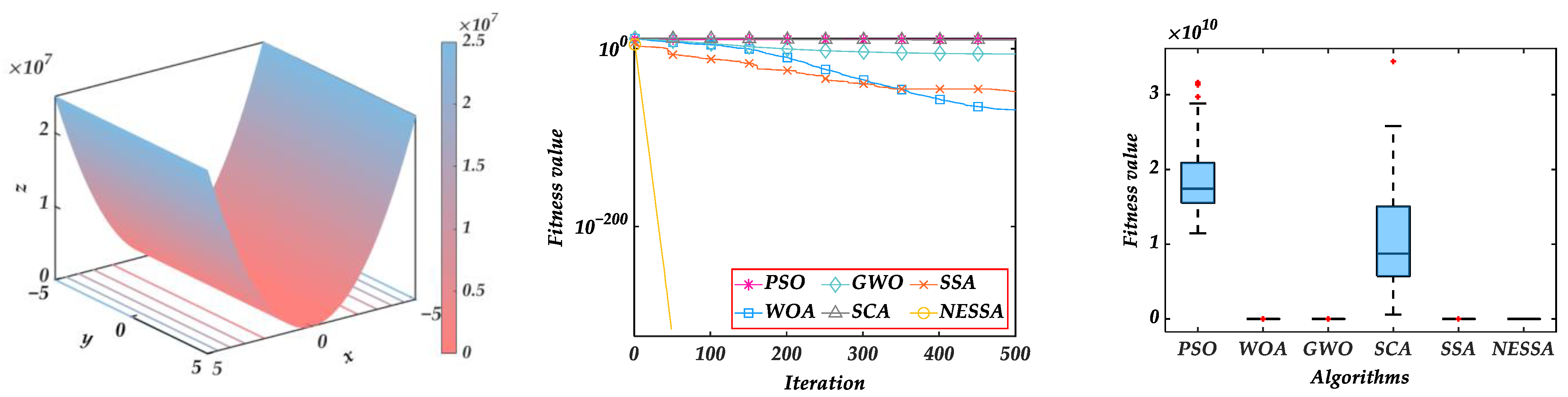
Figure 5.
Sum of Different Powers Function.

Figure 6.
Rotated Hyper–Ellipsoid Function.

Figure 7.
Zakharov Function.

Figure 8.
Sum Squares Function.

Figure 9.
Quartic Function.

Figure 10.
Sphere Model.

Figure 11.
Schwefel’s problem 2.22.

Figure 12.
Schwefel’s problem 1.2.

Figure 13.
Schwefel’s problem 2.21.

Figure 14.
Rastrigin’s Function.

Figure 15.
Ackley’s Function.

Figure 16.
Kowalik’s Function.

Figure 17.
Iterative trajectories of five algorithms.


Figure 18.
Optimization process based on swarm intelligence algorithm.

Figure 19.
Coverage rate curves and boxplots for case 1.

Figure 20.
Node deployment of nine algorithms for case 1.

Figure 21.
Coverage rate curves and boxplots for case 2.

Figure 22.
Node deployment of nine algorithms for case 2.

Figure 23.
Coverage rate curves and boxplots for case 3.

Figure 24.
Node deployment of nine algorithms for case 3.


Table 1.
Benchmark functions.
| Benchmark | Equation | d | Range | Fmin |
|---|---|---|---|---|
| Bent Cigar Function | 100 | [−100, 100] | 0 | |
| Sum of Different Powers Function | 100 | [−100, 100] | 0 | |
| Rotated Hyper–Ellipsoid Function | 100 | [−65, 65] | 0 | |
| Zakharov Function | 100 | [−5, 10] | 0 | |
| Sum Squares Function | 100 | [−10, 10] | 0 | |
| Quartic Function | 100 | [−1.28, 1.28] | 0 | |
| Sphere Model | 100 | [−100, 100] | 0 | |
| Schwefel’s problem 2.22 | 100 | [−10, 10] | 0 | |
| Schwefel’s problem 1.2 | 100 | [−100, 100] | 0 | |
| Schwefel’s problem 2.21 | 100 | [−100, 100] | 0 | |
| Rastrigin’s Function | 100 | [−5.12, 5.12] | 0 | |
| Ackley’s Function | 100 | [−32, 32] | 0 | |
| Kowalik’s Function | 4 | [−5, 5] | 0.000307 |
Table 2.
Test results of six algorithms.
| Benchmark | Result | PSO | WOA | GWO | SCA | SSA | NESSA |
|---|---|---|---|---|---|---|---|
| Mean | 1.8905 × 10¹⁰ | 4.6133 × 10−64 | 1.3138 × 10⁻⁶ | 1.0975 × 10¹⁰ | 5.8424 × 10−45 | 0 | |
| Std. | 5.0627 × 10⁹ | 2.5180 × 10−63 | 1.2085 × 10⁻⁶ | 8.4216 × 10⁹ | 4.1233 × 10−44 | 0 | |
| Time | 0.1162 | 0.1712 | 0.3835 | 0.3062 | 0.9161 | 0.7782 | |
| Mean | 8.9275 × 10⁵ | 1.3847 × 10−67 | 4.9847 × 10⁻¹¹ | 4.9191 × 10⁵ | 6.0385 × 10−41 | 0 | |
| Std. | 2.6495 × 10⁵ | 9.3225 × 10−67 | 4.5438 × 10⁻¹¹ | 3.6447 × 10⁵ | 4.2699 × 10−40 | 0 | |
| Time | 0.0927 | 0.1735 | 0.3772 | 0.2986 | 0.9762 | 0.7717 | |
| Mean | 3.7963 × 10⁵ | 6.6164 × 10−71 | 2.5773 × 10⁻¹¹ | 1.4308 × 10⁵ | 5.9923 × 10−46 | 0 | |
| Std. | 9.1736 × 10⁴ | 2.4545 × 10−71 | 1.7921 × 10⁻¹¹ | 9.7908 × 10⁴ | 4.2372 × 10−45 | 0 | |
| Time | 0.2379 | 0.2991 | 0.5325 | 0.4151 | 1.1570 | 1.0807 | |
| Mean | 6.5223 × 10⁹ | 1.7066 × 10³ | 1.1456 × 10² | 6.7071 × 10² | 9.3710 × 10−44 | 0 | |
| Std. | 4.2494 × 10¹⁰ | 2.9734 × 10² | 5.3017 × 101 | 1.3924 × 10² | 6.6262 × 10−43 | 0 | |
| Time | 0.1069 | 0.1659 | 0.3756 | 0.3171 | 0.8996 | 0.7399 | |
| Mean | 9.0534 × 10³ | 4.3646 × 10−71 | 6.5252 × 10⁻¹³ | 3.5847 × 10³ | 5.1037 × 10⁻³⁴ | 0 | |
| Std. | 2.4400 × 10³ | 3.0630 × 10−70 | 5.7752 × 10⁻¹³ | 23976 × 103 | 3.6089 × 10⁻³³ | 0 | |
| Time | 0.0992 | 0.1761 | 0.3991 | 0.2775 | 0.9566 | 0.8670 | |
| Mean | 1.3882 × 101 | 2.9906 × 10⁻³ | 7.2474 × 10⁻³ | 1.4196 × 10² | 2.9581 × 10⁻⁴ | 7.2163 × 10⁻⁵ | |
| Std. | 6.2807 | 4.1427 × 10⁻³ | 2.3951 × 10⁻³ | 5.7890 × 101 | 2.2796 × 10⁻⁴ | 7.7187 × 10⁻⁵ | |
| Time | 0.3111 | 0.3877 | 0.5716 | 0.5165 | 1.1721 | 0.8637 | |
| Mean | 1.9774 × 10⁴ | 1.9564 × 10−71 | 1.6134 × 10⁻¹² | 1.2025 × 10⁴ | 3.0173 × 10−49 | 0 | |
| Std. | 4.6507 × 10³ | 1.1392 × 10−70 | 1.3372 × 10⁻¹² | 7.9423 × 10³ | 1.5383 × 10−48 | 0 | |
| Time | 0.0850 | 0.1792 | 0.3643 | 0.2922 | 0.9325 | 0.6870 | |
| Mean | 1.3447 × 10² | 5.9195 × 10−49 | 4.2666 × 10⁻⁸ | 9.0974 | 9.1117 × 10⁻²⁹ | 0 | |
| Std. | 2.7261 × 101 | 3.1623 × 10−48 | 1.6837 × 10⁻⁸ | 7.4861 | 5.7121 × 10⁻²⁸ | 0 | |
| Time | 0.0921 | 0.1825 | 0.4209 | 0.2790 | 0.9327 | 0.7957 | |
| Mean | 1.2283 × 10⁵ | 1.0690 × 10⁶ | 6.5699 × 10² | 2.3771 × 10⁵ | 8.2407 × 10−43 | 0 | |
| Std. | 6.4941 × 10⁴ | 2.3307 × 10⁵ | 8.9532 × 10² | 6.0667 × 10⁴ | 5.6712 × 10−42 | 0 | |
| Time | 0.6435 | 0.7011 | 0.8707 | 0.8089 | 1.3878 | 1.1600 | |
| Mean | 3.2619 × 101 | 7.8270 × 101 | 8.8309 × 10⁻¹ | 8.9710 × 10² | 1.7378 × 10⁻²⁹ | 0 | |
| Std. | 3.7684 | 2.3100 × 101 | 8.1956 × 10⁻¹ | 2.7997 | 1.0589 × 10⁻²⁸ | 0 | |
| Time | 0.1178 | 0.1680 | 0.3698 | 0.2757 | 0.8630 | 0.7585 | |
| Mean | 7.5226 × 10² | 0 | 1.0379 × 101 | 2.6752 × 10² | 0 | 0 | |
| Std. | 4.5534 × 101 | 0 | 8.4162 | 1.3756 × 10² | 0 | 0 | |
| Time | 0.1505 | 0.1919 | 0.3981 | 0.3133 | 0.9070 | 0.6757 | |
| Mean | 1.3862 × 101 | 4.2988 × 10⁻¹⁵ | 1.2197 × 10⁻⁷ | 1.8467 × 10² | 8.8818 × 10⁻¹⁶ | 8.8818 × 10⁻¹⁶ | |
| Std. | 8.0286 × 10⁻¹ | 2.3762 × 10⁻¹⁵ | 4.1440 × 10⁻⁸ | 4.6796 | 0 | 0 | |
| Time | 0.1359 | 0.1838 | 0.3957 | 0.3415 | 0.9276 | 0.7167 | |
| Mean | 8.5555 × 10⁻³ | 5.9264 × 10⁻⁴ | 5.4827 × 10⁻³ | 1.0546 × 10⁻³ | 2.3203 × 10⁻³ | 3.2338 × 10⁻⁴ | |
| Std. | 1.3163 × 10⁻² | 3.1154 × 10⁻⁴ | 1.2621 × 10⁻² | 3.8164 × 10⁻⁴ | 6.0756 × 10⁻³ | 1.1952 × 10⁻⁵ | |
| Time | 0.0652 | 0.0783 | 0.0711 | 0.0727 | 0.1702 | 0.2031 |
Table 3.
Wilcoxon p-value test results.
| Benchmark | NESSA vs. PSO | NESSA vs. WOA | NESSA vs. GWO | NESSA vs. SCA | NESSA vs. SSA |
|---|---|---|---|---|---|
| F1 | 3.3111 × 10⁻²⁰ | 3.3111 × 10⁻²⁰ | 3.3111 × 10⁻²⁰ | 3.3111 × 10⁻²⁰ | 4.6715 × 10⁻¹⁹ |
| F2 | 3.3111 × 10⁻²⁰ | 3.3111 × 10⁻²⁰ | 3.3111 × 10⁻²⁰ | 3.3111 × 10⁻²⁰ | 1.6907 × 10⁻¹⁸ |
| F3 | 3.3111 × 10⁻²⁰ | 3.3111 × 10⁻²⁰ | 3.3111 × 10⁻²⁰ | 3.3111 × 10⁻²⁰ | 4.6715 × 10⁻¹⁹ |
| F4 | 3.3111 × 10⁻²⁰ | 3.3111 × 10⁻²⁰ | 3.3111 × 10⁻²⁰ | 3.3111 × 10⁻²⁰ | 1.6907 × 10⁻¹⁸ |
| F5 | 3.3111 × 10⁻²⁰ | 3.3111 × 10⁻²⁰ | 3.3111 × 10⁻²⁰ | 3.3111 × 10⁻²⁰ | 3.3111 × 10⁻²⁰ |
| F6 | 7.0661 × 10⁻¹⁸ | 1.1738 × 10⁻¹⁵ | 7.0661 × 10⁻¹⁸ | 7.0661 × 10⁻¹⁸ | 3.5360 × 10⁻⁹ |
| F7 | 3.3111 × 10⁻²⁰ | 3.3111 × 10⁻²⁰ | 3.3111 × 10⁻²⁰ | 3.3111 × 10⁻²⁰ | 1.6907 × 10⁻¹⁸ |
| F8 | 3.3111 × 10⁻²⁰ | 3.3111 × 10⁻²⁰ | 3.3111 × 10⁻²⁰ | 3.3111 × 10⁻²⁰ | 1.2593 × 10⁻¹⁹ |
| F9 | 3.3111 × 10⁻²⁰ | 3.3111 × 10⁻²⁰ | 3.3111 × 10⁻²⁰ | 3.3111 × 10⁻²⁰ | 4.6715 × 10⁻¹⁹ |
| F10 | 3.3111 × 10⁻²⁰ | 3.3111 × 10⁻²⁰ | 3.3111 × 10⁻²⁰ | 3.3111 × 10⁻²⁰ | 1.2593 × 10⁻¹⁹ |
| F11 | 3.3111 × 10⁻²⁰ | N/A | 3.3111 × 10⁻²⁰ | 3.3111 × 10⁻²⁰ | N/A |
| F12 | 3.3111 × 10⁻²⁰ | 1.1011 × 10⁻¹⁴ | 3.3111 × 10⁻²⁰ | 3.3111 × 10⁻²⁰ | N/A |
| F13 | 1.5991 × 10⁻⁴ | 9.0593 × 10⁻¹⁰ | 1.4307 × 10⁻³ | 1.1417 × 10⁻¹⁷ | 8.7729 × 10⁻⁹ |
Table 4.
Test results of five algorithms.
| Benchmark | Algorithm | Mean | Std. | Time | p-Value |
|---|---|---|---|---|---|
| SSA | 6.1212 × 10−41 | 4.1750 × 10−40 | 9.3090 | 1.6907 × 10⁻¹⁸ | |
| SSASC | 0 | 0 | 12.9206 | N/A | |
| ISSA1 | 4.6707 × 10−80 | 1.7467 × 10−79 | 9.2791 | 7.3684 × 10⁻¹⁶ | |
| ISSA2 | 8.3657 × 10−176 | 3.0297 × 10−175 | 9.2900 | 3.3111 × 10⁻²⁰ | |
| NESSA | 0 | 0 | 7.5399 | ||
| SSA | 3.1521 × 10−42 | 2.9376 × 10−41 | 9.2487 | 4.6715 × 10⁻¹⁹ | |
| SSASC | 0 | 0 | 11.7667 | N/A | |
| ISSA1 | 1.1675 × 10−122 | 7.7152 × 10−121 | 9.5825 | 1.4596 × 10⁻¹² | |
| ISSA2 | 6.7188 × 10−198 | 3.8761 × 10−197 | 9.5071 | 3.3111 × 10⁻²⁰ | |
| NESSA | 0 | 0 | 7.2796 | ||
| SSA | 2.0271 × 10−43 | 1.4299 × 10−42 | 16.5706 | 1.2593 × 10⁻¹⁹ | |
| SSASC | 0 | 0 | 23.7165 | N/A | |
| ISSA1 | 5.3247 × 10−76 | 3.7646 × 10−75 | 12.3822 | 5.2454 × 10⁻¹³ | |
| ISSA2 | 2.8774 × 10−181 | 2.0346 × 10−180 | 13.2727 | 3.3111 × 10⁻²⁰ | |
| NESSA | 0 | 0 | 14.8767 | ||
| SSA | 1.5016 × 10−41 | 9.7589 × 10−41 | 9.3427 | 4.6715 × 10⁻¹⁹ | |
| SSASC | 0 | 0 | 12.7269 | N/A | |
| ISSA1 | 1.9506 × 10−88 | 1.3375 × 10−87 | 9.3298 | 1.4596 × 10⁻¹² | |
| ISSA2 | 4.5823 × 10−182 | 3.2275 × 10−181 | 9.5706 | 3.3111 × 10⁻²⁰ | |
| NESSA | 0 | 0 | 6.9401 | ||
| SSA | 1.8602 × 10⁻³² | 1.3011 × 10⁻³¹ | 9.8776 | 3.3111 × 10⁻²⁰ | |
| SSASC | 0 | 0 | 14.4102 | N/A | |
| ISSA1 | 5.3900 × 10−63 | 3.8108 × 10−63 | 9.1247 | 1.4596 × 10⁻¹² | |
| ISSA2 | 1.5771 × 10−107 | 1.0312 × 10−107 | 9.4143 | 3.3111 × 10⁻²⁰ | |
| NESSA | 0 | 0 | 7.7876 | ||
| SSA | 1.0350 × 10⁻³ | 6.8883 × 10⁻⁴ | 11.0312 | 1.7355 × 10⁻¹⁵ | |
| SSASC | 1.5502 × 10⁻⁴ | 1.3788 × 10⁻⁴ | 15.2722 | 8.5865 × 10⁻⁴ | |
| ISSA1 | 3.6258 × 10⁻⁴ | 2.5674 × 10⁻⁴ | 10.9255 | 9.4565 × 10⁻¹² | |
| ISSA2 | 2.4691 × 10⁻⁴ | 3.0829 × 10⁻⁴ | 11.1934 | 2.8105 × 10⁻¹² | |
| NESSA | 7.7617 × 10⁻⁵ | 6.6362 × 10⁻⁵ | 7.5121 | ||
| SSA | 1.3791 × 10−46 | 9.6292 × 10−46 | 9.0189 | 1.2593 × 10⁻¹⁹ | |
| SSASC | 0 | 0 | 12.5317 | N/A | |
| ISSA1 | 1.3618 × 10−70 | 1.7302 × 10−71 | 9.2598 | 1.4596 × 10⁻¹² | |
| ISSA2 | 3.2087 × 10−163 | 2.2657 × 10−162 | 9.4015 | 3.3111 × 10⁻²⁰ | |
| NESSA | 0 | 0 | 7.2973 | ||
| SSA | 4.3985 × 10⁻²⁵ | 2.6406 × 10⁻²⁴ | 9.2677 | 3.3111 × 10⁻²⁰ | |
| SSASC | 0 | 0 | 13.7007 | N/A | |
| ISSA1 | 8.5571 × 10−38 | 4.5731 × 10−37 | 8.8911 | 7.3687 × 10⁻¹⁶ | |
| ISSA2 | 2.0627 × 10−97 | 1.4497 × 10−96 | 9.0786 | 3.3111 × 10⁻²⁰ | |
| NESSA | 0 | 0 | 7.0836 | ||
| SSA | 5.9257 × 10−37 | 4.1898 × 10−36 | 14.3982 | 4.6715 × 10⁻¹⁹ | |
| SSASC | 0 | 0 | 23.2557 | N/A | |
| ISSA1 | 1.2759 × 10−56 | 9.0185 × 10−55 | 14.3770 | 1.4596 × 10⁻¹² | |
| ISSA2 | 8.7874 × 10−186 | 6.1896 × 10−185 | 15.3228 | 3.3111 × 10⁻²⁰ | |
| NESSA | 0 | 0 | 12.7107 | ||
| SSA | 2.7796 × 10⁻²¹ | 1.4596 × 10⁻²⁰ | 9.1717 | 3.3111 × 10⁻²⁰ | |
| SSASC | 0 | 0 | 13.9827 | N/A | |
| ISSA1 | 1.2358 × 10−61 | 6.1296 × 10−60 | 9.0212 | 2.0607 × 10⁻¹⁷ | |
| ISSA2 | 5.7257 × 10−92 | 4.0786 × 10−91 | 9.1532 | 3.3111 × 10⁻²⁰ | |
| NESSA | 0 | 0 | 6.5867 | ||
| SSA | 0 | 0 | 9.1857 | N/A | |
| SSASC | 0 | 0 | 15.5796 | N/A | |
| ISSA1 | 0 | 0 | 9.3172 | N/A | |
| ISSA2 | 0 | 0 | 9.3216 | N/A | |
| NESSA | 0 | 0 | 6.6278 | ||
| SSA | 8.8818 × 10⁻¹⁶ | 0 | 9.2862 | N/A | |
| SSASC | 8.8818 × 10⁻¹⁶ | 0 | 11.7655 | N/A | |
| ISSA1 | 8.8818 × 10⁻¹⁶ | 0 | 9.1125 | N/A | |
| ISSA2 | 8.8818 × 10⁻¹⁶ | 0 | 9.3269 | N/A | |
| NESSA | 8.8818 × 10⁻¹⁶ | 0 | 6.7362 |
Table 5.
Optimization results for case 1.
| Algorithm | Coverage Rate | p-Value vs. NESSA | Average Time | |||
|---|---|---|---|---|---|---|
| Optimal | Worst | Mean | Std. | |||
| PSO | 0.9771 | 0.9344 | 0.9585 | 1.2067 × 10⁻² | 1.1960 × 10⁻¹² | 11.2371 |
| WOA | 0.9812 | 0.9094 | 0.9521 | 1.6991 × 10⁻² | 1.2019 × 10⁻¹² | 11.5263 |
| GWO | 1.0000 | 0.9906 | 0.9983 | 2.0740 × 10⁻³ | 1.2045 × 10⁻⁷ | 14.1711 |
| SCA | 0.9282 | 0.8607 | 0.8937 | 1.6331 × 10⁻² | 1.2049 × 10⁻¹² | 12.7758 |
| SSA | 0.9563 | 0.8821 | 0.9190 | 2.2586 × 10⁻² | 1.2039 × 10⁻¹² | 15.1322 |
| SSASC | 0.9625 | 0.8533 | 0.9116 | 2.8690 × 10⁻² | 1.2049 × 10⁻¹² | 40.0176 |
| ISSA1 | 0.9823 | 0.8595 | 0.9433 | 2.7137 × 10⁻² | 1.1921 × 10⁻¹² | 14.2296 |
| ISSA2 | 0.9761 | 0.8824 | 0.9205 | 2.2727 × 10⁻² | 1.2198 × 10⁻¹² | 14.8573 |
| NESSA | 1.0000 | 1.0000 | 1.0000 | 0 | 14.7867 | |
Table 6.
Optimization results for case 2.
| Algorithm | Coverage Rate | p-Value vs. NESSA | Average Time | |||
|---|---|---|---|---|---|---|
| Optimal | Worst | Mean | Std. | |||
| PSO | 0.8707 | 0.7619 | 0.8057 | 2.1728 × 10⁻² | 2.8809 × 10⁻¹¹ | 7.1351 |
| WOA | 0.8367 | 0.7607 | 0.7973 | 2.1916 × 10⁻² | 2.9045 × 10⁻¹¹ | 7.4728 |
| GWO | 0.9387 | 0.7437 | 0.9057 | 3.8881 × 10⁻² | 8.7576 × 10⁻⁹ | 7.5063 |
| SCA | 0.7709 | 0.7233 | 0.7421 | 9.9217× 10⁻³ | 2.8287 × 10⁻¹¹ | 6.7501 |
| SSA | 0.7981 | 0.7188 | 0.7572 | 1.8913 × 10⁻² | 2.8827 × 10⁻¹¹ | 8.8687 |
| SSASC | 0.8752 | 0.7528 | 0.8215 | 2.9191 × 10⁻² | 2.8682 × 10⁻¹¹ | 21.6326 |
| ISSA1 | 0.8357 | 0.7486 | 0.7878 | 2.1933 × 10⁻² | 2.8871 × 10⁻¹¹ | 8.6371 |
| ISSA2 | 0.8299 | 0.7211 | 0.7680 | 2.2973 × 10⁻² | 2.8682 × 10⁻¹¹ | 9.1599 |
| NESSA | 0.9523 | 0.9161 | 0.9371 | 9.6561 × 10⁻³ | 7.7711 | |
Table 7.
Optimization results for case 3.
| Algorithm | Coverage Rate | p-Value vs. NESSA | Average Time | |||
|---|---|---|---|---|---|---|
| Optimal | Worst | Mean | Std. | |||
| PSO | 0.9378 | 0.8958 | 0.9171 | 1.2070 × 10⁻² | 2.9972 × 10⁻¹¹ | 195.7561 |
| WOA | 0.9507 | 0.8888 | 0.9264 | 1.4455 × 10⁻² | 2.9953 × 10⁻¹¹ | 201.8856 |
| GWO | 0.9925 | 0.9687 | 0.9818 | 5.7332 × 10⁻³ | 1.8486 × 10⁻¹⁰ | 207.3233 |
| SCA | 0.8756 | 0.7897 | 0.8337 | 1.5766 × 10⁻² | 2.9953 × 10⁻¹¹ | 197.1167 |
| SSA | 0.8862 | 0.8271 | 0.8636 | 1.2899 × 10⁻² | 2.9935 × 10⁻¹¹ | 208.3121 |
| SSASC | 0.9411 | 0.7082 | 0.8532 | 6.1694 × 10⁻² | 3.0161 × 10⁻¹¹ | 702.6788 |
| ISSA1 | 0.9447 | 0.8913 | 0.9156 | 1.3141 × 10⁻² | 2.9972 × 10⁻¹¹ | 216.7396 |
| ISSA2 | 0.9207 | 0.8522 | 0.8770 | 1.3337 × 10⁻² | 3.0161 × 10⁻¹¹ | 219.6671 |
| NESSA | 0.9957 | 0.9885 | 0.9927 | 1.8950 × 10⁻³ | 202.7887 | |
Publisher’s Note: MDPI stays neutral with regard to jurisdictional claims in published maps and institutional affiliations. |
© 2022 by the authors. Licensee MDPI, Basel, Switzerland. This article is an open access article distributed under the terms and conditions of the Creative Commons Attribution (CC BY) license (https://creativecommons.org/licenses/by/4.0/).
Share and Cite
MDPI and ACS Style
Liu, R.; Mo, Y. Performance of a Novel Enhanced Sparrow Search Algorithm for Engineering Design Process: Coverage Optimization in Wireless Sensor Network. Processes 2022, 10, 1691. https://doi.org/10.3390/pr10091691
AMA Style
Liu R, Mo Y. Performance of a Novel Enhanced Sparrow Search Algorithm for Engineering Design Process: Coverage Optimization in Wireless Sensor Network. Processes. 2022; 10(9):1691. https://doi.org/10.3390/pr10091691
Chicago/Turabian StyleLiu, Rui, and Yuanbin Mo. 2022. "Performance of a Novel Enhanced Sparrow Search Algorithm for Engineering Design Process: Coverage Optimization in Wireless Sensor Network" Processes 10, no. 9: 1691. https://doi.org/10.3390/pr10091691
Note that from the first issue of 2016, this journal uses article numbers instead of page numbers. See further details here.