
Research on Position Control of an Electro–Hydraulic Servo Closed Pump Control System
by
Fei Wang
1,2,
Gexin Chen
1,2,*,
Huilong Liu
1,
Guishan Yan
1,
Tiangui Zhang
1,
Keyi Liu
2,
Yan Liu
2 and
Chao Ai
1 1
School of Mechanical Engineering, Yanshan University, Qinhuangdao 066004, China
2
Mechanical and Electrical Engineering, Xinjiang Institute of Engineering, Urumqi 830023, China
*
Author to whom correspondence should be addressed.
Processes 2022, 10(9), 1674; https://doi.org/10.3390/pr10091674
Submission received: 8 August 2022
/
Revised: 16 August 2022
/
Accepted: 19 August 2022
/
Published: 23 August 2022
Abstract
:A control strategy combining adaptive backstep sliding mode control and dead-zone inverse compensation control in a series was proposed to solve the problem of system parameter uncertainty and system dead-zone in the process of position control in an electro–hydraulic servo closed pump control system. Firstly, an adaptive backstepping sliding mode controller was designed by introducing the sliding mode control principle. Secondly, the smooth dead-zone inverse function was constructed by using the smooth continuous index function to design the dead-zone inverse compensation controller, which is combined with the adaptive sliding mode controller to form a series controller. Finally, the feasibility of the controller was verified by using the pump control servo system of a lithium battery pole strip mill. The experimental results show that, compared with traditional PID control, the control strategy displayed no excessive overshoot before the steady state, the steady-state control accuracy could reach ±0.002 mm, and the time required to reach the steady state was 1 s to 2 s shorter, which shows this method’s ability to effectively improve the position control accuracy of the pump control system, as well as its dynamic response performance.
1. Introduction
The electro–hydraulic servo pump control system is a highly integrated driving unit composed of a servo motor, a quantitative pump, a hydraulic cylinder, a functional valve group, etc. Due to its advantages of high efficiency and environmental protection, high power weight ratio, low cost and strong bearing capacity [1,2], the system is widely used in national defense and industrial fields, such as aircraft steering systems [3], ship and submarine steering systems [4], and traditional control systems such as construction machinery [5]. At the same time, it is becoming more widely used in emerging and expanding fields, such as automobiles [6] and bionic robots [7]. In recent years, with the development and maturity of high-magnetic-energy rare earth permanent magnet materials and advanced manufacturing technology, high-speed piston pumps, intelligent materials, active flow distribution and other technologies have been continuously applied to the composition of pump-controlled servo systems, and the rapidity and stability of the entire actuation system have been greatly improved. At the same time, the compactness and response frequency of the actuation system have been significantly improved [8,9]. Electro–hydraulic servo pump control technology has become a popular research direction in the field of electro–hydraulic servos.
In the position control process of the electro–hydraulic servo pump control system, due to the perturbation of parameters such as the elastic modulus of the system oil, the flow leakage coefficient, the viscous friction coefficient of the hydraulic cylinder, the equivalent spring stiffness of the load and the disturbance of the external load, the system presents strong nonlinear characteristics [10]. At present, most experts and scholars employ feedback linearization [11], sliding mode control [12,13,14,15], adaptive control [16,17,18], fuzzy control [19,20] and other technologies to address the influence of transient time-varying parameters and nonlinear factors [21,22,23] in electro–hydraulic position servo systems. Among them, adaptive control combined with backstepping easily deals with the uncertain and unknown parameters in the system, so it has been studied and applied by many scholars. Kaddissi et al. [24] used the regression least square method to estimate the uncertain parameters of the online system, designed an indirect adaptive backstepping controller based on the output estimated value, and conducted a comparative experiment with the nonadaptive backstepping controller. The experimental results showed that the controller can still track the expected reference signal with slight transient behavior after parameter changes. The nonadaptive controller will lead to large oscillations and instability in the system. Ba et al. [25] proposed an integrated model inversion controller for pump control electro–hydraulic systems based on the integrated model inversion method to solve the uncertainty and nonlinearity of the hydraulic actuator system. The experimental results showed that the designed controller has high controllability. Chen et al. [26] proposed a nonlinear adaptive step control strategy based on the backstepping method, and established the uncertainty parameter adaptive rate to adjust the parameter disturbance in real time, which improved the accuracy and robustness of the control system.
Although adaptive backstepping control can effectively solve the problem of unmatched uncertainty in the system, the problem of nesting between the control law designed by this method and the parameter adaptive law is common, which affects the control performance of the system. The sliding mode control method has complete adaptability to external disturbances and parameter perturbations in the control system, and can maintain good robustness when the system’s uncertainties meet the matching conditions. Yin et al. [27] proposed a new electro–hydraulic servo pitch system, which integrated an adaptive robust integral sliding mode pitch angle controller and a projection adaptive law to accurately track the desired pitch angle trajectory and compensate for model uncertainty and uncertain interference. The proposed controller and adaptive law showed good performance in practice. Yang et al. [28] proposed a novel sliding mode control design framework for the position tracking control of a hydrostatic actuation system (EHSAS), which was composed of three sub-modules: the reduced order model of EHSAS, the disturbance sliding mode observer (DSMO) and the new adaptive arrival law (NARL). DSMO was used to estimate and compensate for the mismatched interference in the reduced order model, which improved the transient performance, steady-state accuracy and robustness of the position control of the system.
During the initial operation and low-speed control of the pump control system, the output of the system lagged behind, and the system dead-zone arose due to the internal oil leakage and compression of the system. The existence of a dead-zone can easily lead to problems such as control accuracy reduction, dynamic quality degradation and system instability [29]. Most of the research on the dead-zone compensation of nonlinear systems equates the dead-zone to the disturbance of the system, and uses a robust controller to suppress it. Kokotovic [30] proposed to integrate the dead-zone compensation mechanism into the adaptive controller design process in the valve control system in the early years, and verified it through simulation experiments. American scholar Mohanty [31] and Portuguese scholar Coelho [32] also incorporated the dead-zone compensation mechanism into their designed control algorithms and verified them. However, the dead-zone model, analyzed by the dead-zone compensation mechanism studied by the three scholars above, is discontinuous, and involves the risk of causing chattering in the control system. Zhou et al. [33] introduced the concept of the dead-zone smooth inverse function and used it in the design of an adaptive controller based on backstepping technology. Experiments showed that this method can ensure the stability of the control system. Yao et al. [34] considered the influence factors of the dead-zone characteristics of the electro–hydraulic servo system on position control, and established a method of combining adaptive control and dead-zone inverse compensation control into a series controller to improve the system control accuracy.
It can be seen from the above that for the parameter uncertainty of the system and the dead-zone of the system in the position control process of the electro–hydraulic servo closed pump control system, scholars have carried out relevant research from the single aspect of adaptive backstepping control, sliding mode control and dead-zone compensation or the combination of the two, but there is no research literature combining the three at the same time. In this paper, a control strategy combining the adaptive backstep sliding mode control and dead-zone inverse compensation control is proposed. The parameter adaptive law is used to adjust uncertain parameter disturbance online in real time, and the smooth dead-zone inverse function is used to compensate the dead-zone of the system, which reduces the influence of parameter error on the control performance and improves the accuracy of position control of the pump control system. The control strategy provides a reference for the research on the position control of the electro–hydraulic servo closed pump control system.
2. Principle of Pump Control System
The electro–hydraulic servo pump control system studied in this paper is mainly composed of electrical and hydraulic parts, and its working principle is shown in Figure 1. The hydraulic part is composed of a servo motor, a constant displacement pump, an oil replenishment module and an execution unit. The system uses the servo motor to drive the constant displacement pump coaxially. The suction and discharge ports of the constant displacement pump are directly connected to the two load ports of the hydraulic cylinder. The accumulator cooperates with the one-way valve to replenish oil in the system, and the overflow valve acts as a safety valve to prevent the system pressure from exceeding the safety limit. The electrical part is composed of a state feedback device, a computer control module and a servo driver. The state feedback device collects the displacement signal of the piston rod of the hydraulic cylinder, the computer control module processes the signal, and the controller outputs the speed command to the servo motor and adjusts the output speed in real time by controlling the input voltage of the servo motor, thereby adjusting the output pressure and flow of the fixed displacement pump. Finally, this controls the output displacement of the piston of the hydraulic cylinder.
3. Mathematical Model
Based on the above pump control system, the mathematical models of key hydraulic components were established [26,27].
3.1. Servo Motor
In the process of position control in the pump control system, in this paper, the servo motor, as the execution terminal of the control algorithm, is the core component. The servo motor converts the control input voltage into the output speed of the motor. Considering the high response speed and control accuracy of the servo motor, the relationship between the output speed of the motor and the input control signal can be regarded as a proportional loop, which is expressed as follows:
where is the output speed of the motor, is the control gain, and is the input voltage signal.
3.2. Fixed Displacement Pump
Considering oil compression, internal and external leakage and other factors, we analyzed the flow distribution characteristics of the quantitative pump, as shown in Figure 2.
The two-cavity load volume flow from the pump to the controlled hydraulic cylinder can be expressed as follows:
where is the flow in cavity A of the system, is the flow in cavity B of the system, is the displacement of the displacement pump, is the pressure in cavity A of the system, is the pressure in cavity B of the system, is the internal leakage coefficient of the displacement pump, and is the external leakage coefficient of the displacement pump.
3.3. Double-Acting Symmetrical Hydraulic Cylinder
Considering load conditions, oil compression, internal and external leakage and other factors, the flow distribution characteristics of the hydraulic cylinder were analyzed, and the flow continuity equation of the two chambers of the hydraulic cylinder is established as follows:
where is the efficient working area of the hydraulic cylinder, is the displacement of the hydraulic cylinder, is the effective bulk modulus, is the compression volume of the hydraulic cylinder’s cavity A, is the compression volume of the hydraulic cylinder’s cavity B, is the internal leakage coefficient of the hydraulic cylinder and is the external leakage coefficient of the hydraulic cylinder.
Formula (3) can be simplified as:
where is the total compression volume.
The force balance equation of the hydraulic cylinder is as follows:
where is the total mass converted from the load to the piston of the hydraulic cylinder, is the viscous damping coefficient of the oil, is the equivalent spring stiffness of the load and is the external interference and unmodeled friction force.
The block diagram of the closed-pump control system can be established using the Laplace transformation expressed in Equations (1)–(3) and (5), as shown in Figure 3.
Substituting the Laplace transformation expressed in Equations (1), (2) and (5) into Equation (4) yields:
where .
We select the output speed of the servo motor as the model input vector, that is, .
If we define the system state vector as piston rod displacement , piston rod speed , and piston rod speed , then the state vector can be written as:
According to Formulas (1)–(5), the strict feedback form of the state equation of the nonlinear model of the electro–hydraulic servo pump control system can be expressed as:
where we define the variables as follows:
Therefore, Equation (8) can be expressed as:
where .
4. Controller Design
The problem of nesting between the control law and the parameter adaptive law of adaptive backstepping control design is common, and this affects the control performance of the system [33]. In addition, the dead-zone of the pump control system will affect the closed-loop response characteristics of the system, resulting in a series of problems such as delayed response, poor tracking performance and large impact. In this paper, the principle of sliding mode control is introduced to design an adaptive backstepping sliding mode controller. Adaptive backstepping control and sliding mode control are used to eliminate the influence of system mismatching and matching uncertainties, and avoid the occurrence of nested problems. At the same time, in order to avoid the output chattering problem of the dead-zone inverse compensator caused by the unsmooth dead-zone inverse function, the smooth dead-zone inverse function is designed by using the smooth continuous index function, and the dead-zone inverse compensation controller is designed based on this function. The series position controller composed of adaptive backstepping sliding mode controller and dead-zone inverse compensator is applied to the pump control system. The pump control system series control framework is shown in Figure 4.
4.1. Adaptive Backstepping Sliding Mode Controller
The adaptive backstepping control method has great advantages in solving the problem of the unmatched uncertainty of the system. The sliding mode control method can maintain good robustness when the system uncertainties meet the matching conditions. Therefore, the adaptive backstepping sliding mode control, which combines the advantages of the two, has become an effective scheme to deal with the uncertainty of the system, and the introduction of sliding mode control avoids the nesting problem between the adaptive rate of parameters and the control output based on the backstepping method, while also further improving the control performance.
The design process of the adaptive backstepping sliding mode controller is as follows:
- 1.
- Step 1
Since the control objective of the electro–hydraulic servo pump control system is that the actual output position better reproduce the expected value, the position tracking error is defined as:
where is the expected value of the state variable . Subsequently, the derivative of with respect to time is as follows:
Next, is defined as the state deviation between state variable and its expected value .
An alternate Lyapunov function is defined as follows:
Subsequently, the derivative of with respect to time is as follows:
According to Equation (15), when , there is . However, because is the deviation between and , cannot contain . Hence, is defined as
where is a positive constant. Substituting Equation (16) into Equation (15) yields:
The aforementioned formula indicates that when is zero, is negative semidefinite, and the tracking error converges to zero. Therefore, the next task is to design a control law to make close to zero or as small as possible.
- 2.
- Step 2
Taking the derivative of and with respect to time gives the following:
We define a new alternate Lyapunov function as follows:
Subsequently, the derivative of with respect to time is as follows:
Substituting Equation (19) into Equation (21) yields:
Next, is defined as the state deviation between state variable and its expected value .
According to the same analysis of Equation (16),
where is a positive constant. Substituting Equation (24) into Equation (22) yields:
The aforementioned equation indicates that when is zero, is negative semidefinite. Therefore, the next task is to design a control law to make close to zero, or as small as possible.
- 3.
- Step 3
The combination of adaptive control and sliding mode control is used to solve the problem of nesting in the process of adaptive rate design. The sliding mode switching function is defined at the third step of the adaptive backstepping controller design, as:
where and are the sliding surface positive constants.
The derivation of Equation (26) with respect to time is as follows:
When the system state slides on the sliding surface, we get , so . In order to avoid the effect of control on the designed parameter adaptation rate, the Lyapunov function is constructed as:
Subsequently, the derivation of Equation (28) with respect to time is as follows:
We define the variables as follows: ,,,,. Therefore, Equation (29) can be expressed as:
The adaptive control strategy is used to predict the parameters , , , and . We define the parameter error , where , and is the estimated value of .
We define the system Lyapunov function as follows:
where is the parameter adaptive gain of parameter .
The derivation of Equation (31) with respect to time is as follows:
Therefore, the adaptive sliding mode controller can be designed as:
where is a positive constant. Substituting Equation (33) into Equation (32) yields:
The parameter adaptation rate is obtained as:
Substituting Equation (35) into Equation (34) yields:
where .
For the Lyapunov function of the system shown in Equation (31), constructed by Equations (14), (20) and (28), the controller and parameter adaptation rate shown in Equations (33) and (35) are adopted in the design. If the parameters , , , and satisfy the inequality shown in Equation (37), then the first- to third-order sequential principal minors of matrix Q are greater than zero, so Q is a positive definite matrix.
Therefore, Equation (36) shows that ; because and are bounded, is also bounded. According to Barbalat’s lemma, can be obtained, making the whole system asymptotically stable.
4.2. Dead-Zone Inverse Compensation Controller
In the electro–hydraulic servo pump control system, due to the combined action of the hydraulic pump, the overflow valve and one-way valve leakage, the hydraulic cylinder static friction and other factors, the system output appears to be the dead-zone, which is called “system dead-zone”. In the process of system analysis, it is more reliable to analyze the dead-zone characteristics of the input and output of the measurement system, and the compensation with “system dead-zone” is also more practical in engineering practice.
Although the dead-zone inverse function of general nonlinear systems can also realize the dead-zone inverse compensation function, most of the dead-zone functions of nonlinear systems are not smooth, and the dead-zone inverse compensation controller designed with this kind of function will inevitably produce a certain chattering phenomenon. In this paper, dead-zone compensation control is realized by constructing a smooth dead-zone inverse. The nonlinear dead-zone inverse function is processed with a smooth continuous index function to obtain a new smooth dead-zone inverse function [35], and the dead-zone inverse compensation controller is designed based on this function.
- 1.
- Compensation principle
The system model is as shown in Equation (38) [33]:
where is the system state variable, is the linear and nonlinear function containing the system state parameters, is the input of the system, and are the unknown constant, and is the output of the system. The actuator nonlinearity is described as a dead-zone characteristic, and is the output of the controller.
The control objective of dead-zone inverse compensation is to design an output feedback control law for the controller output to ensure that all closed-loop signals are bounded, and make the system output track the given reference signal in the following assumptions.
Hypothesis 1.
The sign of b is known, and its first n derivatives are known and bounded.
Hypothesis 2.
The dead-zone parametersandsatisfyand, whereandare two small positive numbers.
The dead-zone characteristic [29] can be expressed as shown in Figure 5 and Equation (39):
where , , and are constants. In general, the breakpoint is and the slope is .
The purpose of compensating the dead-zone effect is to use the dead-zone inverse [36], so the smooth continuous index function is used to construct the smooth dead-zone inverse function:
where and are smooth continuous index functions, which are defined as follows [33]:
where and . Smooth dead-zone inversion is shown in Figure 6:
We parameterize dead-zone characteristic :
where , and . and are defined as follows:
Since is unknown and is unavailable, the actual control input of the system is designed as:
where is the estimated value of , as follows:
Therefore, the corresponding control output is expressed as:
The error between and is as follows:
where . Subsequently, we obtain the bound of as follows:
where .
When , the boundary of decreases with the increase or decrease in . Therefore, is bounded for all , and when and converge asymptotically to zero, the also converges asymptotically to zero.
- 2.
- Design process
This paper relies on the pump-controlled AGC system of a lithium battery pole strip mill as the experimental platform for this measurement, and adopts the following “system dead-zone” measurement method [37]. Firstly, initially, the hydraulic cylinder is placed at the fully retracted position point, and the controller outputs a 0.0005 v/ms incremental voltage signal to the servo motor, monitors and records the relationship between the extension displacement of the hydraulic cylinder piston and the input voltage, and obtains the positive dead-zone curve of the system, as shown in Figure 7. Next, we change the initial position of the hydraulic cylinder piston to the fully extended position point, use the control to output the decreasing voltage signal of 0.0005 mv/ms to the servo motor, monitor and record the relationship between the hydraulic cylinder piston extension displacement and the input voltage, and obtain the negative dead-zone curve of the system, as shown in Figure 8.
Parameters , , and can be obtained from Figure 7 and Figure 8, and the system dead-zone inverse compensation controller can be obtained by substitution into Equations (40) and (41).
Finally, the system dead-zone inverse compensation controller is combined with the adaptive backstepping sliding mode controller to form the system series control, as shown in Figure 4.
5. Engineering Experiment Results and Analysis
5.1. Engineering Experiment Elatform
Based on the pump control servo system of the lithium battery pole strip mill, this paper experimentally studies the series controller composed of an adaptive backstepping sliding mode controller and a dead-zone inverse compensator. The rolling mill equipment uses the hydraulic gap thickness automatic control equipment (referred to as hydraulic AGC) to adjust the gap between the upper and lower rolls, then compacts the battery pole pieces, uses the motor to drive the upper and lower rolls to rotate, spins and pulls the battery pole pieces under the action of friction, and completes the pole piece rolling process.
The rolling mill pump control AGC is composed of the main computer MITSUBISHI PLC, the communication protocol converter, a MOOG MSCII motion controller, a Beckhoff module, a servo driver, a motor pump unit and a hydraulic system. The pump-controlled AGC hydraulic system is installed on both sides of the lower roll of the rolling mill, as shown in Figure 9. The system highly integrates the EPU, hydraulic cylinder and other hydraulic accessories through the functional valve block.
Figure 10 shows the AGC control structure of the mill pump control, in which the control software adopts the MOOG (New York, USA) axis control software MACS 3.4, and the control hardware is composed of an Advantech (Taiwan, China) IPC-600 computer, Beckhoff (Weil, Germany) modules EK1100, EL3122 and EL2004, a host computer MOOG controller MSD, a MOOG single-axis servo driver and other auxiliary components. The PC of the device uses MACS 3.4 to write the main control program, imports the main computer MSD through TCP/IP, sends the control signal to the servo driver by EtherCAT communication and receives the feedback signal of the hydraulic system collected by the Beckhoff module at the same time.
5.2. Experiment Analysis
In order to more intuitively present the control effect of the adaptive backstepping sliding mode and dead-zone inverse compensation control algorithm proposed in this paper, it is compared and analyzed with PID control in the rolling mill pump control AGC. The main parameters of the rolling mill pump control AGC are shown in Table 1.
At the beginning of the design of the lithium battery pole piece rolling mill system, the pump-controlled AGC is installed at the lower roll in order to compress the pump-controlled AGC hydraulic cylinder to the fully retracted state, relying on the weight of the roll and tooling machinery when the system is unloaded. Therefore, the experiment only yields a rising “S” slope trajectory signal. The “S” slope trajectory shows displacements of 0.1 mm from 82.06 mm to 82.16 mm, 0.05 mm from 82.06 mm to 82.11 mm, and 0.01 mm from 82.06 mm to 82.07 mm and displacement and error curves are obtained, as shown in Figure 11 and Figure 12.
It can be seen from Figure 11 and Figure 12 that there is a certain gap in the adjustment of the traditional PID control parameters for different working conditions, so it is difficult to adapt a group of optimal parameters to all working conditions, and the steady-state accuracy of the system is relatively poor. When the displacement is 0.1 mm and 0.05 mm, it reaches ±0.008 mm, and when the displacement is 0.01 mm, it reaches ±0.006 mm. The series controller based on an adaptive backstepping sliding mode controller and a dead-zone inverse compensation controller does not display too much overshoot before entering the steady state. The steady-state control accuracy can reach ±0.002 mm, and the time to reach the steady state is 1 to 2 s shorter than with the traditional PID control. Therefore, according to the above experimental results, it can be determined that the series control method proposed in this paper has significantly improved the position control performance and dynamic response characteristics of the pump-controlled AGC system, as well as realizing the high-performance position control of this system.
6. Conclusions
Using adaptive backstep sliding mode control theory and dead-zone inverse compensation theory, the system parameter uncertainty and system dead-zone problems that rise in the position control of an electro–hydraulic servo closed pump control system were studied. The conclusions are as follows:
- The mathematical model of the electro–hydraulic servo pump control system was established, and the position output transfer function of the system was deduced.
- Based on the backstepping recursion criterion, an adaptive backstepping sliding mode controller was designed by introducing the sliding mode control principle, and the dead-zone inverse compensation controller was designed by constructing a smooth dead-zone inverse function. Then the two controllers formed a system series controller and were applied to the position control of the pump control system.
- Experimental analysis shows that the control strategy proposed in this paper yields good control performance in practical applications. Compared with the traditional PID control, there is no excessive overshoot before the steady state, the steady-state control accuracy can reach ±0.002 mm, and the time required to reach the steady state is 1–2 s shorter.
However, the structure of the series controller designed in this paper is relatively complex, and it needs to be further optimized for specific projects. In addition, this paper uses the concept of “system dead-zone” measurement and calibration to compensate the whole system, which can be used to further study the dead-zone mechanism of each unit of the pump control system, and further improve its control accuracy.
Author Contributions
Funding acquisition, F.W. and T.Z.; formal analysis, F.W.; methodology, G.C., H.L. and G.Y.; project administration, G.Y. and C.A.; resources, G.C., G.Y. and H.L.; software, K.L. and Y.L.; writing—original draft, F.W. and H.L.; writing—review and editing, G.C. and G.Y.; supervision, F.W. and G.C. All authors have read and agreed to the published version of the manuscript.
Funding
This research was funded by the Key R&D Projects in Hebei Province (No. 20314402D), the Key Project of Science and Technology Research in Hebei Province (No. ZD2020166; No. ZD2021340), the Project supported by the Natural Science Foundation of Xinjiang Uygur Autonomous Region (2022D01A51) and the Project of Scientific Research Plan of Colleges and Universities in Xinjiang Uygur Autonomous Region (XJEDU2021Y050), The central government guides local science and technology development special fund projects(ZYYD2022C09).
Institutional Review Board Statement
Not applicable.
Informed Consent Statement
Not applicable.
Data Availability Statement
Not applicable.
Conflicts of Interest
The authors declare no conflict of interest.
References
- Hong, W.; Wang, S.; Tomovic, M.M.; Liu, H.; Shi, J.; Wang, X. A Novel Indicator for Mechanical Failure and Life Prediction Based on Debris Monitoring. IEEE Trans. Reliab. 2017, 66, 161–169. [Google Scholar] [CrossRef]
- Lu, C.; Wang, S.; Makis, V. Fault Severity Recognition of Aviation Piston Pump Based on Feature Extraction of EEMD Paving and Optimized Support Vector Regression Model. Aerosp. Sci. Technol. 2017, 67, 105–117. [Google Scholar] [CrossRef]
- Guo, S.; Chen, J.; Lu, Y.; Wang, Y.; Dong, H. Hydraulic piston pump in civil aircraft: Current status future directions and critical technologies. Chin. J. Aeronaut. 2020, 33, 16–30. [Google Scholar] [CrossRef]
- Xu, C.; Liu, G.; Xu, G.; Li, F.; Zhai, Y. The depth and pitch control of submarines based on the pump-hydraulic servo. Chin. J. Ship Res. 2017, 12, 116–123. [Google Scholar]
- Li, Y.; Fan, R.; Yang, L.; Zhao, B.; Quan, L. Research status and development trend of intelligent excavators. Mech. Eng. 2020, 56, 165–178. [Google Scholar]
- Lee, J.; Oh, K.; Yi, K. A novel approach to design and control of an active suspension using linear pump control-based hydraulic system. Proc. Inst. Mech. Eng. Part D J. Automob. Eng. 2020, 234, 1224–1248. [Google Scholar] [CrossRef]
- Grimminger, F.; Meduri, A.; Khadiv, M.; Viereck, J.; Wüthrich, M.; Naveau, M.; Righetti, L. An open torque-controlled modular robot architecture for legged locomotion research. IEEE Robot. Autom. Lett. 2020, 5, 3650–3657. [Google Scholar] [CrossRef]
- Chaudhuri, A.; Wereley, N. Compact hybrid electro–hydraulic actuators using smart materials: A review. J. Intell. Mater. Syst. Struct. 2012, 23, 597–634. [Google Scholar] [CrossRef]
- Song, Y.; Tai, M.; Wang, R.; Chen, L.; Zhu, Y. Experimental research on a dual magnetostrictive axial plunger pumps-based electro-hydrostatic actuator. Chin. Hydraul. Pneum. 2020, 7, 36–41. [Google Scholar]
- Jing, C.; Xu, H.; Jiang, J. Dynamic Surface Disturbance Rejection Control for Electro–Hydraulic Load Simulator. Mech. Syst. Signal Process. 2019, 134, 106293–106306. [Google Scholar] [CrossRef]
- Sani, S.; Chaji, A. Output Feedback Nonlinear Control of Double-Rod Hydraulic Actuator using Extended Kalman Filter. In Proceedings of the IEEE 4th International Conference on Knowledge-Based Engineering and Innovation (KBEI), Tehran, Iran, 22–22 December 2017; pp. 0349–0354. [Google Scholar]
- Zad, H.S.; Ulasyar, A.; Zohaib, A. Robust Model Predictive Position Control of Direct Drive Electro–Hydraulic Servo System. In Proceedings of the 2016 International Conference on Intelligent Systems Engineering (ICISE), Islamabad, Pakistan, 15–17 January 2016. [Google Scholar]
- Ji, X.; Wang, C.; Chen, S.; Zhang, Z. Sliding mode backstepping control method for valve-controlled electro–hydraulic Position Servo System. J. Cent. South Univ. Sci. Technol. 2020, 51, 1518–1525. [Google Scholar]
- Ji, X.; Wang, C.; Zhang, Z.; Chen, S.; Guo, X. Nonlinear adaptive position control of hydraulic servo system based on sliding mode back-stepping design method. Proc. Inst. Mech. Eng. 2021, 235, 0349–0354. [Google Scholar] [CrossRef]
- Han, S.; Jiao, Z.; Wang, C.; Shang, Y.; Shi, Y. Fractional integral sliding mode nonlinear control of electro–hydraulic flight turntable. J. Beijing Univ. Aeronaut. Astronaut. 2014, 40, 1411–1416. [Google Scholar]
- Helian, B.; Chen, Z.; Yao, B.; Yu, L.; Li, C. Accurate Motion Control of a Direct-drive Hydraulic System with an Adaptive Nonlinear Pump Flow Compensation. IEEE ASME Trans. Mechatron. 2020, 26, 2593–2603. [Google Scholar] [CrossRef]
- Tri, N.M.; Nam, D.N.C.; Park, H.G.; Ahn, K.K. Trajectory control of an electro hydraulic actuator using an iterative backstepping control scheme. Mechatronics 2015, 29, 96–102. [Google Scholar] [CrossRef]
- Shang, X.; Zhou, H.; Yang, H. Research Status of Active Control Method for Fluid Pulsation in Hydraulic System. J. Mech. Eng. 2019, 55, 216–226. [Google Scholar]
- Zhu, Y.; Sun, Y.; Chen, G. Simulation Research on Hydraulic Loading System of Wind Turbine Based on Particle Swarm PID Control. In Proceedings of the IEEE Conference on Telecommunications, Optics and Computer Science (TOCS), Shenyang, China, 11–13 December 2020; pp. 385–388. [Google Scholar]
- Liem, D.T.; Truong, D.Q.; Park, H.G.; Ahn, K.K. A Feedforward Neural Network Fuzzy Grey Predictor-based Controller for Force Control of an Electro–hydraulic Actuator. Int. J. Precision Eng. Manuf. 2016, 17, 309–321. [Google Scholar] [CrossRef]
- Guo, P.; Li, Y.; Li, J.; Zhang, B.; Wu, X. Design of primary mirror position control system for large aperture telescope. Acta Opt. Sin. 2020, 40, 122–128. [Google Scholar]
- Maghareh, A.; Silva, C.E.; Dyke, S.J. Parametric model of servo-hydraulic actuator coupled with a nonlinear system: Experimental validation. Mech. Syst. Signal Process. 2018, 104, 663–672. [Google Scholar] [CrossRef]
- Hao, Y.; Xia, L.; Gem, L.; Wang, X.; Quan, L. Research on position control characteristics of hybrid linear drive system. Trans. Chin. Soc. Agric. Mach. 2020, 51, 379–385. [Google Scholar]
- Kaddissi, C.; Kenne, J.P.; Saad, M. Indirect Adaptive Control of an Electrohydraulic Servo System Based on Nonlinear Backstepping. IEEE/ASME Trans. Mechatron. 2011, 16, 1171–1177. [Google Scholar] [CrossRef]
- Ba, D.X.; Ahn, K.K.; Truong, D.Q.; Park, H.G. Integrated model-based backstepping control for an electro–hydraulic system. Int. J. Precis. Eng. Manuf. 2016, 17, 565–577. [Google Scholar] [CrossRef]
- Chen, G.; Liu, H.; Jia, P.; Qiu, G.; Yu, H.; Yan, G.; Zhang, J. Position Output Adaptive Backstepping Control of Electro–Hydraulic Servo Closed-Pump Control System. Processes 2021, 9, 2209. [Google Scholar] [CrossRef]
- Yin, X.; Zhang, W.; Jiang, Z.; Pan, L. Adaptive robust integral sliding mode pitch angle control of an electro–hydraulic servo pitch system for wind turbine. Mech. Syst. Signal Process. 2019, 133, 105704. [Google Scholar] [CrossRef]
- Yang, R.; Fu, Y.; Zhang, L.; Qi, H.; Han, X.; Fu, J. A Novel Sliding Mode Control Framework for Electrohydrostatic Position Actuation System. Math. Probl. Eng. 2018, 2018, 7159891. [Google Scholar] [CrossRef]
- Wang, Y.; Tian, R. Analysis and Compensation for Nonlinear Systems with Dead-zone. Ind. Control Appl. 2006, 4, 64–66. [Google Scholar]
- Tao, G.; Kokotovic, P.V. Adaptive control of plants with unknown dead-zones. IFAC Proc. Vol. 1994, 39, 59–68. [Google Scholar]
- Mohanty, A.; Yao, B. Integrated Direct/Indirect Adaptive Robust Control of Hydraulic Manipulators with Valve Deadband. IEEE/ASME Trans. Mechatron. 2011, 16, 707–715. [Google Scholar] [CrossRef]
- dos Santos Coelho, L.; Cunha, M.A.B. Adaptive Cascade Control of a Hydraulic Actuator with an Adaptive Dead-Zone Compensation and Optimization Based on Evolutionary Algorithms. Expert Syst. Appl. 2011, 38, 12262–12269. [Google Scholar] [CrossRef]
- Zhou, J.; Wen, C.; Zhang, Y. Adaptive Output Control of Nonlinear Systems with Uncertain Dead-Zone Nonlinearity. IEEE Trans. Autom. Control 2006, 51, 504–511. [Google Scholar] [CrossRef]
- Gu, W.; Yao, J.; Yao, Z.; Zheng, J. Robust Adaptive Control of Hydraulic System with Input Saturation and Valve Dead-Zone. IEEE Access 2018, 6, 53521–53532. [Google Scholar] [CrossRef]
- Chowdhury, F.N.; Wahi, P.; Raina, R.; Kaminedi, S. A Survey of Neural Networks Applications in Automatic Control. In Proceedings of the 33rd Southeastern Symposium on System Theory, Athens, OH, USA, 20–20 March 2001; pp. 349–353. [Google Scholar]
- Li, Y.; Mao, Z.Z.; Wang, F.L.; Wang, Y. Adaptive dead zone compensation control of electrode regulating system of electric arc furnace. Control Decis. 2010, 25, 1474–1478. [Google Scholar]
- Wang, L.; Zhao, D.; Liu, F.; Liu, Q.; Zhang, Z. ADRC for Electro–hydraulic Position Servo Systems Based on Dead-zone Compensation. China Mech. Eng. 2021, 32, 1432–1442. [Google Scholar]
Figure 1.
Schematic diagram of electro–hydraulic servo closed-pump control system. 1: servo motor; 2: fixed displacement pump; 3/4: one-way valve; 5: accumulator; 6/7: one-way valve; 8/9: solenoid directional valve; 10: hydraulic cylinder. A and B represent the two chambers of the oil cylinder respectively.
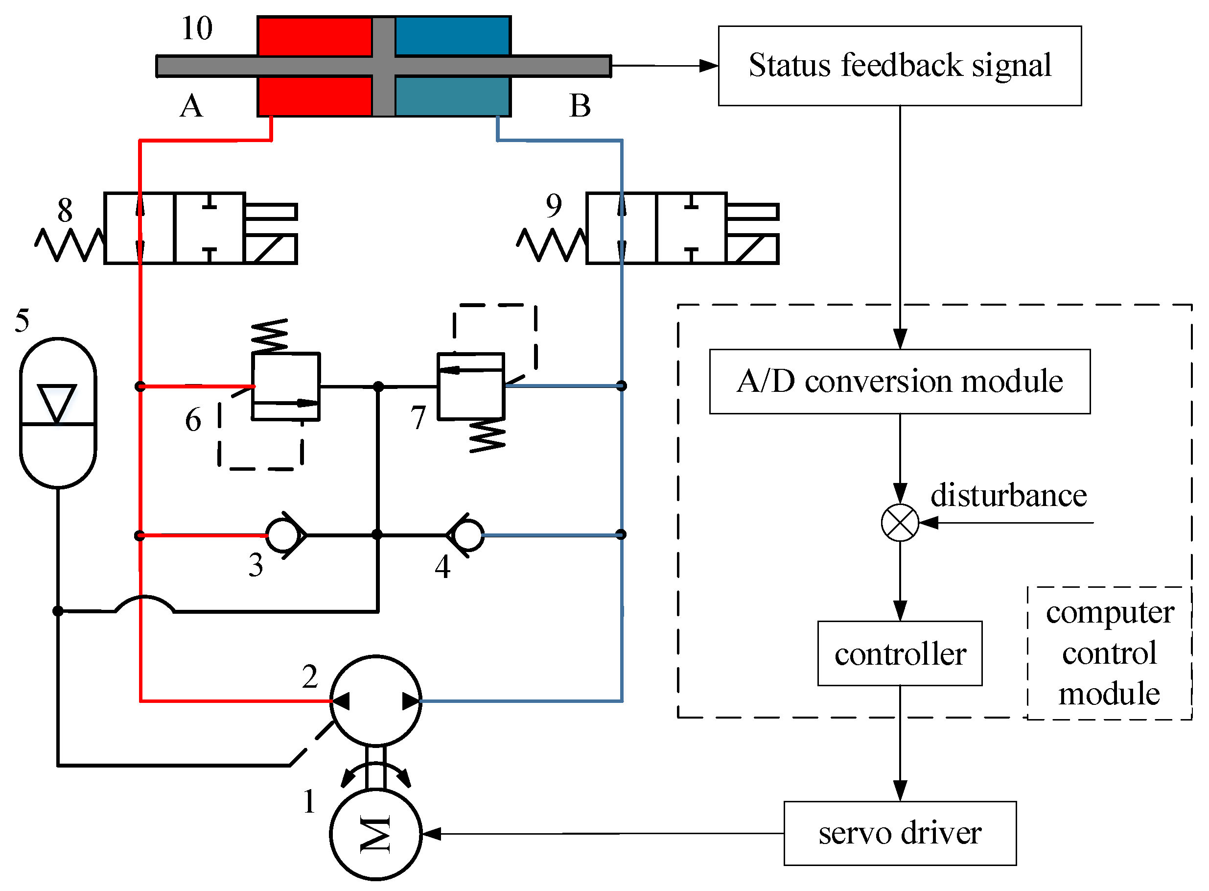
Figure 2.
Flow distribution of hydraulic pump.

Figure 3.
Block diagram of pump control system.

Figure 4.
Series control block diagram of pump control system.
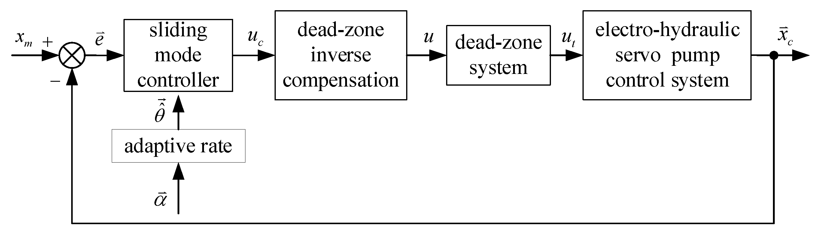
Figure 5.
Dead-zone characteristic curve.

Figure 6.
Smooth dead-zone inverse curve.

Figure 7.
System positive dead-zone curve. The red line is the displacement curve of the hydraulic cylinder in the positive dead-zone of the system, and the blue line is the reference line based on the compensation principle, which is used to obtain the estimated parameters of the dead-zone.
Figure 7.
System positive dead-zone curve. The red line is the displacement curve of the hydraulic cylinder in the positive dead-zone of the system, and the blue line is the reference line based on the compensation principle, which is used to obtain the estimated parameters of the dead-zone.
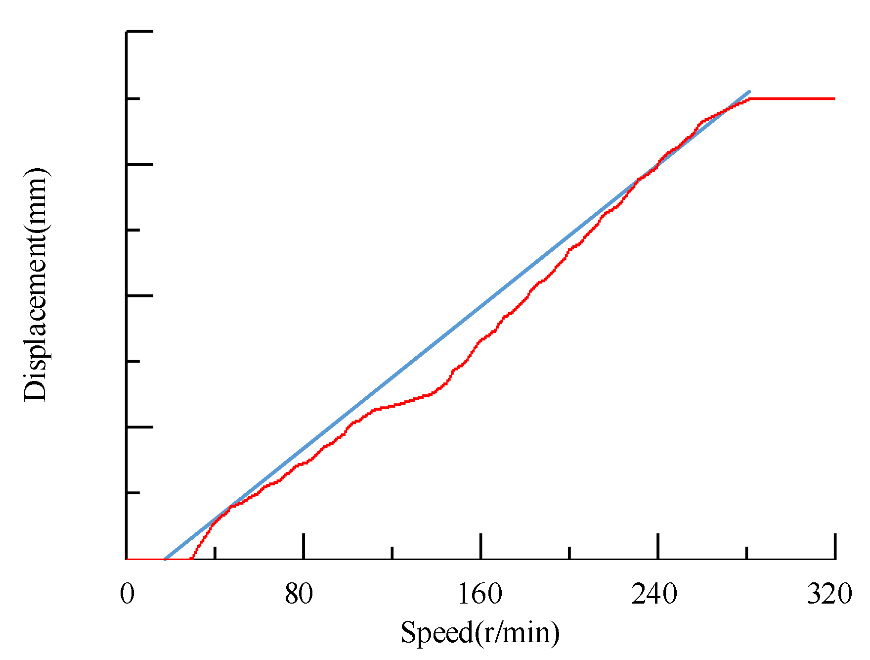
Figure 8.
System negative dead-zone curve. The red line is the displacement curve of the hydraulic cylinder in the negative dead-zone of the system, and the blue line is the reference line based on the compensation principle, which is used to obtain the estimated parameters of the dead-zone.
Figure 8.
System negative dead-zone curve. The red line is the displacement curve of the hydraulic cylinder in the negative dead-zone of the system, and the blue line is the reference line based on the compensation principle, which is used to obtain the estimated parameters of the dead-zone.
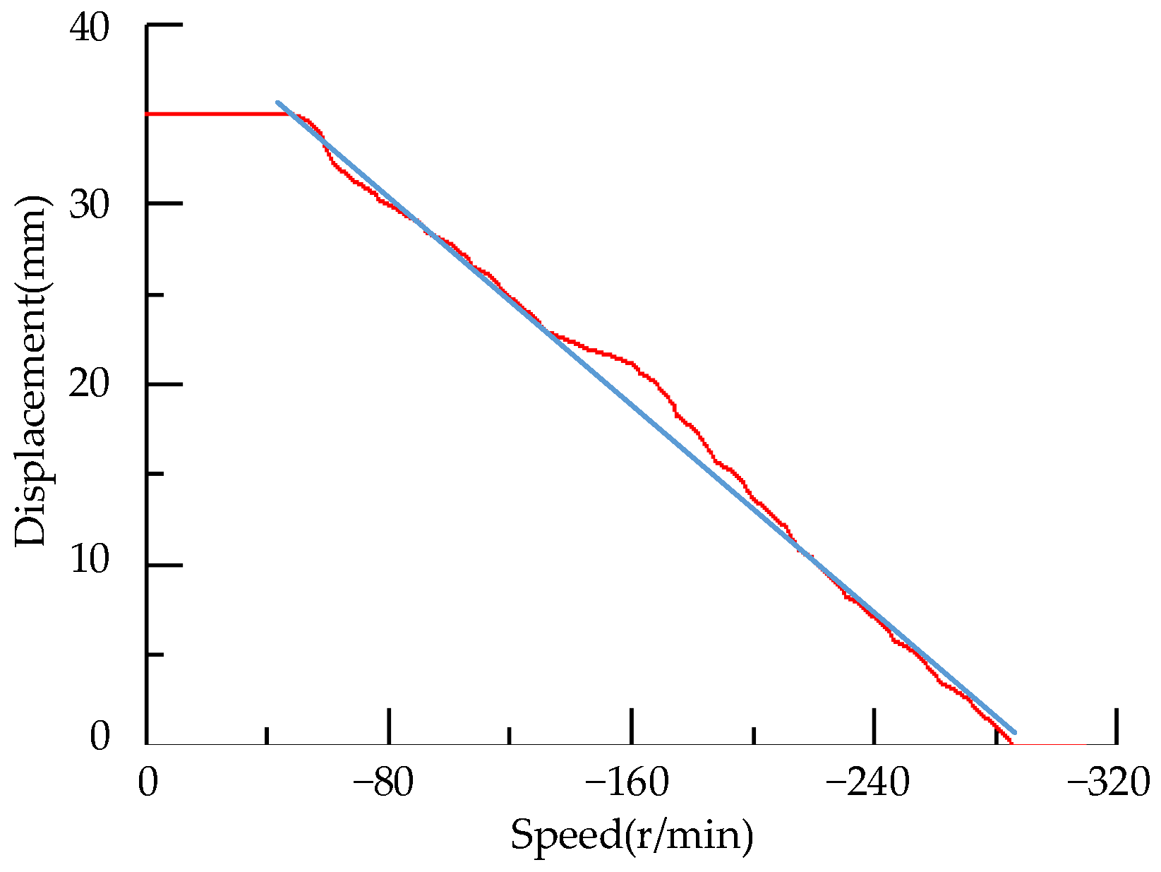
Figure 9.
Experimental platform.

Figure 10.
Rolling mill pump control AGC control frame.

Figure 11.
Displacement tracking curve. (a) Displacement 0.1 mm; (b) displacement 0.05 mm; (c) displacement 0.01 mm.
Figure 11.
Displacement tracking curve. (a) Displacement 0.1 mm; (b) displacement 0.05 mm; (c) displacement 0.01 mm.

Figure 12.
Error curve. (a) Error with displacement of 0.1 mm; (b) error with displacement of 0.05 mm; (c) error with displacement of 0.01 mm.
Figure 12.
Error curve. (a) Error with displacement of 0.1 mm; (b) error with displacement of 0.05 mm; (c) error with displacement of 0.01 mm.


Table 1.
Operating parameters of experimental platform.
| Parameter | Symbol | Units | Value |
|---|---|---|---|
| Total compression volume | 9.15 × 10⁻⁴ | ||
| Efficient working area cylinder | 0.1134 | ||
| Total mass converted from the load to the piston | 500 | ||
| Viscous damping coefficient | N/(m/s) | 150 | |
| Equivalent spring stiffness of the load | N/m | 9 × 10⁷ | |
| Total leakage coefficient of hydraulic system | (m3/s)/Pa | 9 × 10⁻¹¹ | |
| Effective volume modulus of oil | N/m2 | 6.5 × 10⁸ | |
| Control gain | (r/min)/V | 200 | |
| Displacement of fixed displacement pump | L/r | 8 × 10⁻³ | |
| External disturbance and unmodeled friction | 4× 10⁴ |
Publisher’s Note: MDPI stays neutral with regard to jurisdictional claims in published maps and institutional affiliations. |
© 2022 by the authors. Licensee MDPI, Basel, Switzerland. This article is an open access article distributed under the terms and conditions of the Creative Commons Attribution (CC BY) license (https://creativecommons.org/licenses/by/4.0/).
Share and Cite
MDPI and ACS Style
Wang, F.; Chen, G.; Liu, H.; Yan, G.; Zhang, T.; Liu, K.; Liu, Y.; Ai, C. Research on Position Control of an Electro–Hydraulic Servo Closed Pump Control System. Processes 2022, 10, 1674. https://doi.org/10.3390/pr10091674
AMA Style
Wang F, Chen G, Liu H, Yan G, Zhang T, Liu K, Liu Y, Ai C. Research on Position Control of an Electro–Hydraulic Servo Closed Pump Control System. Processes. 2022; 10(9):1674. https://doi.org/10.3390/pr10091674
Chicago/Turabian StyleWang, Fei, Gexin Chen, Huilong Liu, Guishan Yan, Tiangui Zhang, Keyi Liu, Yan Liu, and Chao Ai. 2022. "Research on Position Control of an Electro–Hydraulic Servo Closed Pump Control System" Processes 10, no. 9: 1674. https://doi.org/10.3390/pr10091674
Note that from the first issue of 2016, this journal uses article numbers instead of page numbers. See further details here.