Data Driven Model Estimation for Aerial Vehicles: A Perspective Analysis

Abstract

Unmanned Aerial Vehicles (UAVs) are important tool for various applications, including enhancing target detection accuracy in various surface-to-air and air-to-air missions. To ensure mission success of these UAVs, a robust control system is needed, which further requires well-characterized dynamic system model. This paper aims to present a consolidated framework for the estimation of an experimental UAV utilizing flight data. An elaborate estimation mechanism is proposed utilizing various model structures, such as Autoregressive Exogenous (ARX), Autoregressive Moving Average exogenous (ARMAX), Box Jenkin’s (BJ), Output Error (OE), and state-space and non-linear Autoregressive Exogenous. A perspective analysis and comparison are made to identify the salient aspects of each model structure. Model configuration with best characteristics is then identified based upon model quality parameters such as residual analysis, final prediction error, and fit percentages. Extensive validation to evaluate the performance of the developed model is then performed utilizing the flight dynamics data collected. Results indicate the model’s viability as the model can accurately predict the system performance at a wide range of operating conditions. Through this, to the best of our knowledge, we present for the first time a model prediction analysis, which utilizes comprehensive flight dynamics data instead of simulation work.

1. Introduction

Over the past few decades, UAVs have become an emerging resource for remote sensing of various precision, agricultural, military, civil [1], and industrial applications [2,3]. The rapidly increasing fleet of UAVs, along with the widening sphere of their utility, therefore presents a serious challenge for the designers to formulate unique optimal control strategies. However, technological advancements in the aviation sector [4,5,6,7] and ground control vehicles [8,9,10,11,12,13,14,15,16,17,18,19] paved the way for the development of hi-fidelity systems. These UAVs help researchers by providing means to collect multi-spectral information with limited resources and data collection times which is critical for time sensitive dynamic data [20]. The pivotal factor for a successful and safe remote sensing research/mission is a robust and fault tolerant UAV control system. Linear and Non-linear control strategies have been used in diverse ways for solving varying control problems to achieve desired objectives [21,22,23,24]. Developing such control systems require well-characterized dynamic system models. Similar work [25,26] has been done in the field of ground robotics [8,9,10,11,12,13,27] as well. Wind tunnel testing (commonly used method for determining the parameters of these dynamic systems) is time-consuming and costly. System Identification (SI) can be used to overcome the limitation of analytical and wind tunnel testing methods for UAVs. There are several techniques in system identification which can be applied to develop dynamic system models and identify model parameters. These methods have been applied to various aerial vehicles in recent years. The developed dynamic model can further be used to design and verify the autopilot control system of the UAV.

1.1. Related Work

Despite their military importance and abundant usage, owing to the proprietary nature of these UAVs, very little information related to design and development is available in literature. Appreciable research work on design and optimization of quad-copters and UAVs has been done by Mir et al. [22,23]. However, the research work available on model identification and optimization of UAVs usually covers one or two techniques of system identification. Perspective analysis and comparison of various techniques on UAVs are quite sparse. Hopping et al. [28] has used a grey box modeling approach applying the prediction estimation method (PEM) to model longitudinal dynamics of a UAV named Taurus.

Mir et al. [29] has further done a tremendous contribution towards soaring energetics of a bio-inspired UAVs. Design optimization of a variable-span morphing wing UAVs and other design optimization and controllability schemes for UAVs have been discussed in detail by Mestrinho et al. & Mir et al. [30,31]. Later, the lateral dynamics of the same UAV was modeled using the same approach and technique by Ahsan et al. [32]. Longitudinal and lateral dynamics of SmartOne UAV were modeled by Rasheed [33] using grey box modeling approach with prediction error method along with performance of error analysis.

Belge et al. [34] obtains an estimate of UAV lateral dynamic system response by using empirical input-output data sets. The accuracy of parametric model estimation (using ARX, ARMAX and OE model structures) and model degrees are compared for different external disturbance effects. The model of Load Transporting System (LTS) originally designed on UAV has been obtained by linear ARX model structure by Altan et al. [35]. ARX system identification model has also been used to identify Multiple Input Multiple Output (MIMO) model of a helicopter. Various transfer functions have been used to analyze the flight dynamics of helicopter. The system identification of a quad rotor-based aerial manipulator is presented in research carried out by Dube and Pedro [36]. ARX and ARMAX models have been obtained from linear accelerations and yaw angular accelerations.

Cavanini et al. [37] has proposed a novel online estimation technique using LPV-ARX model which is both cost effective and storage effective. His method permits to improve the base of knowledge of the provided LS-SVM by introducing the possibility to learn from on-line data, neglecting to perform the time-expensive training phase, such that the proposed approach is suitable for on-line execution. Cavanini et al further [38] presents a Model Predictive Control (MPC) based autopilot for a fixed-wing Unmanned Aircraft Vehicle (UAV) for meteorological data sampling tasks, named Aerosonde. The LPV model is used to design a MPC to drive the UAV. Two different data driven Linear Parameter-Varying MPC (MPCLPV) algorithms have been proposed by using a subspace identification technique. Belge et al. [39] performs the optimum path planning and tracking using Harris hawk optimization (HHO)–grey wolf optimization (GWO), a hybrid metaheuristic optimization algorithm, to enable the UAV to actualize the payload hold–release mission avoiding obstacles. His novel approach generates a fast and safe optimal path without becoming stuck with local minima, and the quad copter tracks the generated path with minimum energy and time consumption. Weng et al. [40] addresses the robust trajectory tracking control problem of disturbed quadrotor UAVs with disturbances, uncertainties and unmodeled dynamics by devising a novel compound robust tracking control (CRTC) approach via data-driven cascade control technique. Marc et al. [41] presents the online updating of the flight envelope of a UAV. His technique is data-driven and the UAV is subjected to structural degradation for the research.

Yu et al. [42] investigates the problem of neural adaptive distributed formation control for quad rotor multiple UAVs subject to unmodeled dynamics and disturbance. Saengphet et al. [43] uses the input and output data obtained from a flight mission of a tail-less UAV for SISO mathematical model using frequency response. Bnhamdoon et al. [44] uses Box-Jenkins model structure and presents a novel method of identification of a quad-copter autopilot system under noisy circumstances.Real time identification of quad-rotor UAV dynamics using a deep learning techniques for has also been studied by Ayyad et al. [45]. Another online estimation method for UAV, using Extended Kalman Filter(EKF) technique has been presented by Mungguia et al. [46].Puttige and Anavatti [47] uses both online and offline models of nonlinear and complex UAV have been obtained using system identification procedure based on Artificial Neural Network (ANN).

Wu et al. [48] provides an approximated solution of the graph partitioning problem by using a deterministic annealing neural network algorithm. The algorithm is a continuation method that attempts to obtain a high-quality solution by following a path of minimum points of a barrier problem as the barrier parameter is reduced from a sufficiently large positive number to 0. A survey of different methods of system identification techniques and its applications for small low-cost aerial vehicles has been carried out by Mir et al. [6,7] and Hoffer et al. [49]. The different control-oriented models of a quad-rotor UAV have been obtained by applying different identification methods presented by Sierra and Santos [50]. Comparison of ARX method for linear estimation and Hammerstein -Wiener method for non linear estimation for ARF-60 UAV identified models is presented by Khalil and Yesildirek [20].

In addition to above referred literature, there are numerous other contributions made by different researchers. Most of the literature is focused on fixed-winged or multi-rotor UAVs used for research work in the fields of military (target drown, target interceptor, aerial munition practice) and non-military (search and rescue, area surveillance, environmental, agriculture) applications. Even for UAVs, the field of side-by-side comprehensive analysis and comparison of different linear and non-linear system identification techniques still has a vast potential for research.

1.2. Motivating Problems for This Paper

Model prediction and performance analysis using experimental flights for UAVs or other aerial vehicles is not feasible due to the involved cost and damage hazard to the system and the environment in case of any crash. Although wind tunnel testing and CFD analysis for model prediction and performance analysis can be done, however, system identification presents a very cost-effective and user friendly solution towards mathematical modelling of the aerial vehicles. Based on the literature review, it has been observed that in-spite of system identification being widely used for UAVs, very little work related to model prediction of UAV using system identification is available. Even in UAVs, the comparison of predicted models using different linear and non linear methods is yet to be explored. The authors of this paper felt that the researchers must be provided with a platform for comparison of linear and non-linear techniques using actual flight data for model estimation and validation. This lack of literature for UAV model prediction using actual flight data motivated the author to fill in this gap through this paper.

1.3. Main Contributions of This Paper

As evident from the preamble of related work, very little research is available in open literature which is based on elaborate comparison of different techniques of system identification for UAVs. Most of the literature for model prediction of UAVs is based on simulation results rather than utilizing actual flight data. Furthermore, when it comes to UAVs, the research contribution using actual flight data along with comprehensive performance evaluation and comparison of linear and nonlinear system identification techniques is even much scarce.

The authors aim to present a base platform for model prediction of UAV utilizing actual flight data after a comprehensive perspective analysis of linear and nonlinear system identification techniques. This paper aims to provide a consolidated platform for the audience which provides a mechanism for model prediction of UAV/UAVs. Besides providing a comprehensive affect of individual training of actual flight data, the presented approach will also help the readers to carry out analysis of several regression techniques in linear and non-linear domain. Moreover, the performance comparison of linear and nonlinear system identification models for quality parameters like final prediction error, residual analysis, mean squared errors and fit percentages further enhances the effectively of the proposed approach.

1.4. Sequence of This Paper

This paper is organized as follows. Section 2 presents the build up of 6-Degree of Freedom (DOF) aerodynamic model for UAV followed by design parameters of UAV. Then a brief overview of all system identification used in this research is given. The results and analysis part gives first presents the flight sorties design conducted for estimation and validation purposes followed by the response of all linear and nonlinear parametric model along with residue analysis of each. A detailed analysis and comparison is carried out for selection of final model. Then the author has also verified the finally selected model by predicting a second actual flight of UAV. Lastly, the conclusion and limitations of the research are presented.

2. Problem Formulation

2.1. 6 DOF Flight Dynamics Model

A 6-Degrees of Freedom (DOF) Flight Dynamics Model (FDM) has been used for studying the motion of UAV in three dimensions. 6DOF refers to the number of axes that a rigid body may freely move in three-dimensional space. It specifies the number of independent factors that define the configuration of a mechanical system. The body may move in three dimensions, on the X, Y, and Z axes, as well as change orientation between those axes via rotation known as pitch, yaw, and roll. FDM assumes a flat and non-rotating earth approximations and is based on dynamic equations (deduced by Stevens, Lewis and Johnson [51]) in body frame reference. These sets of equations, which govern dynamics of translation (Equation (1)), rotation (Equation (2)), kinematics (Equation (3)) and navigation (4)) respectively, are defined as:-

$$\begin{array}{cc}\hfill \dot{U}& =RV-QW-gsin\theta +\frac{X_A+X_T}{m}\hfill \\ \hfill \dot{V}& =-RU+PW+gsin\varphi cos\theta +\frac{Y_A+Y_T}{m}\hfill \\ \hfill \dot{U}& =QU-PV+gcos\varphi cos\theta +\frac{Z_A+Z_T}{m}\hfill \end{array}$$

(1)

In Equation (1), $\dot{U}$, V, W are the components of linear velocities along the three body axes respectively. $\varphi ,\theta$&$\psi$ are the Euler angles which define the orientation of body frame with respect to inertial frame, P, Q, R are the angular velocities along body x, y and z axis respectively. $X_A,Y_A,Z_A$ & $X_T,Y_T,Z_T$ are the Force and Thrust components along the three axis.

$$\begin{array}{cc}\hfill \Gamma \dot{P}& =J_{XZ}(J_X-J_Y+J_Z)PQ\hfill \\ \hfill & -[J_Z(J_Z-J_Y)+J_{XZ}^2]QR+J_{Z}l+J_{XZ}n\hfill \\ \hfill \Gamma \dot{Q}& =(J_Z-J_X)PR-J_{XZ}(P^2-R^2)+m\hfill \\ \hfill \Gamma \dot{P}& =[J_X(J_X-J_Y)+J_{XZ}^2]PQ-J_{XZ}(J_X-J_Y+J_Z)QR\hfill \\ \hfill & +J_{XZ}l+J_{X}n\hfill \end{array}$$

(2)

where $J_X,J_y,J_z,J_{XZ}$ and $\Gamma$ are the inertia matrix components. Also $l,m,n$ are the roll, pitch and yaw moments.

$$\begin{array}{cc}\hfill \dot{\varphi }& =P+tan\theta (Qsin\varphi +Rcos\varphi )\hfill \\ \hfill \dot{\theta }& =Qcos\varphi -Rsin\varphi \hfill \\ \hfill \dot{\psi }& =\frac{Qsin\varphi +Rcos\varphi }{cos\theta }\hfill \end{array}$$

(3)

$$\begin{array}{cc}\hfill \dot{P_E}& =Ucos\theta cos\psi +V(-cos\varphi sin\psi +sin\varphi sin\theta cos\psi )\hfill \\ \hfill & +W(sin\varphi sin\psi +cos\varphi sin\theta cos\psi )\hfill \\ \hfill \dot{P_N}& =Ucos\theta sin\psi +V(cos\varphi cos\psi +sin\varphi sin\theta sin\psi )\hfill \\ & +W(-sin\varphi cos\psi +cos\varphi sin\theta sin\psi )\hfill \\ \hfill \dot{h}& =Usin\theta -Vsin\varphi cos\theta -Wcos\varphi cos\theta \hfill \end{array}$$

(4)

where $P_e$ and $P_n$ are the position coordinates alongside the inertial east and north directions. h is the vehicle altitude, J is the moment of inertia matrix, m is the mass, g is the acceleration due to gravity, l, m, n are the angular velocity components (roll, pitch and yaw moments) in the body axis, $\alpha$ and $\beta$ are the aerodynamic angles representing angle of attack and side slip angle respectively.

Aerodynamic Parameters

High fidelity numerical techniques of Computational Fluid Dynamics (CFD) and USAF DATCOM were utilized for generating FDM based on 6-DOF simulation environment. Flight conditions define aerodynamic forces and moments acting on high speed and are governed by Equations (5) and (6) respectively.

$$\begin{array}{c}\hfill L=q_{\infty }S{C}_L,D=q_{\infty }S{C}_D,Y=q_{\infty }S{C}_Y\end{array}$$

(5)

where L, D and Y represent aerodynamic lift, drag and side force respectively in wind axis. $C_L,C_D,C_Y$ are the dimensionless aerodynamic coefficients for lift, drag and side forces respectively, $q_{\infty }$ is the dynamic pressure and S is the wing area.

$$l_w=q_{\infty }bS{C}_l,m_W=q_{\infty }cS{C}_m,n_W=q_{\infty }bS{C}_n$$

(6)

where $n_w$, $m_w$ and $l_w$ are the yaw, pitch and roll moments in wind axis, b is the wing span, c is the wing chord and $C_n,C_m,C_l$ are the dimensionless aerodynamic coefficients for yaw, pitch and roll moments respectively. The design of UAV under test was optimized based on CFD analysis and comparison of various design configurations.

3. Model Identification

The objective of this search is to build an accurate model for UAV. MATLAB was used for system identification of the system. The adopted research methodology was divided into following steps:

• Acquiring data for two sorties of experimental UAV.
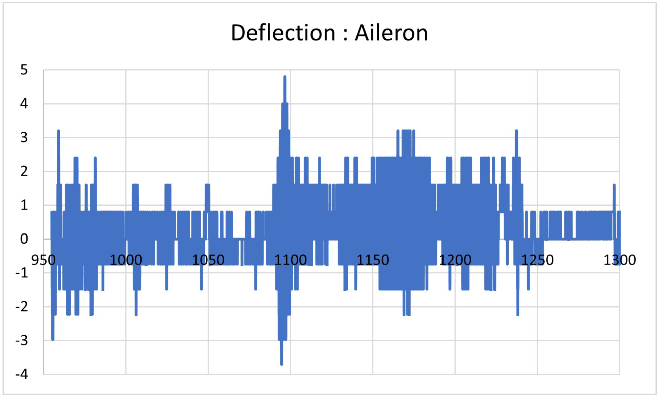
• Pre-processing and filtering the data for whole flight of the UAV.
• Model identification using flight data from one sortie using ARX, ARMAX, Output Error, Box Jenkin’s, Non-linear ARX (with various estimators).
• Training of model for each individual technique
• Selection of best fit model on basis of model quality parameters like Final Prediction Error (FPE), fit percentage to actual flight data and residual analysis.
• Validation of selected model on a different flight data and analysis of the results.

3.1. Model Structures

Various model structures are used in this research to model MIMO dynamics of the UAV. The inputs taken were aileron deflection (${\delta }_a$) and Vtail deflection (${\delta }_e$) whereas the outputs are taken to be yaw rate (P), pitch rate (Q), and roll rate (R).

3.1.1. Auto-Regressive Exogenous (ARX) Model

The second method used is the estimation of ARX model which as per the literature is assumed to be the most efficient polynomial estimation method as linear regression equations are in analytic form whose solution is also unique. The estimation of the ARX model is the most efficient of the polynomial estimation methods because it is the result of solving linear regression equations in analytic form with a unique solution. when the model order is high, then ARX model is preferred. For input $u\left(t\right)$, output $y\left(t\right)$ and noise $e\left(t\right)$, the ARX model is given by Equation (7).

$$\begin{array}{c}\hfill A\left(q\right)y\left(t\right)=\sum _{i=0}^{nu}{B}_i\left(q\right)u_i(t-n{k}_i)+e\left(t\right)\end{array}$$

(7)

where A and B are polynomials expressed in time shift operator $q^{-1}$. Although ARX model is suited for most high order dynamic systems, it has a disadvantage as the disturbances are part of the system model. The disadvantage of the ARX model is that disturbances are part of the system dynamics. However, this disadvantage can be curbed with a good signal-to-noise ratio.

3.1.2. Auto Regressive Moving Average eXogenous (ARMAX) Model

For dynamics systems with dominating disturbances that enter the process in the early stages like wind gust in case of aerial systems, ARMAX model comes in handy. ARMAX model has advantage over ARMAX model by providing more flexibility for handling disturbances.For input $u\left(t\right)$, output $y\left(t\right)$ and noise $e\left(t\right)$, the ARMAX model is given by Equation (8).

$$\begin{array}{c}\hfill A\left(q\right)y\left(t\right)=\sum _{i=0}^{nu}{B}_i\left(q\right)u_i(t-n{k}_i)+C\left(q\right)e\left(t\right)\end{array}$$

(8)

where A, B and C are polynomials expressed in time shift operator $q^{-1}$.

3.1.3. Box Jenkin’s (BJ) Model

When complete system model dynamics are described by modeling the noise and system dynamics separately, this comes under the category of BJ’s Model.Very sparse literature is available related to research carried out on UAVs using BJ model as this model is particularly useful when the disturbances enter towards the end of the process. The disturbance is basically the measurement noise. For input $u\left(t\right)$, output $y\left(t\right)$ and noise $e\left(t\right)$, the BJ model is given by Equation (9).

$$\begin{array}{c}\hfill y\left(t\right)=\sum _{i=0}^{nu}\frac{B_i\left(q\right)}{F_i\left(q\right)}{u}_i(t-n{k}_i)+\frac{C\left(q\right)}{D\left(q\right)}e\left(t\right)\end{array}$$

(9)

where B, C, D and F are polynomials expressed in time shift operator $q^{-1}$.

3.1.4. Output Error (OE) Model

Output Error model is usually used when there is only the need to parameterize the system dynamics without estimating the noise model. This model is only suitable for theoretical modelling of the aerial vehicles, however, its use in practical system dynamics may be considered after due consideration. For input $u\left(t\right)$, output $y\left(t\right)$ and noise $e\left(t\right)$, the OE model is given by Equation (10).

$$\begin{array}{c}\hfill y\left(t\right)=\sum _{i=0}^{nu}\frac{B_i\left(q\right)}{F_i\left(q\right)}{u}_i(t-n{k}_i)+e\left(t\right)\end{array}$$

(10)

3.1.5. State Space Model

State Space model structure was also used in this research owing to its less computational time in case of iterative analysis which can be attributed to lower model order of the state space model. Equation (11) describes a state space system.

$$\begin{array}{c}\hfill x(t+1)=Ax\left(t\right)+Bu\left(t\right)+Ke\left(t\right)\\ \hfill y\left(t\right)=Cx\left(t\right)+Du\left(t\right)+e\left(t\right)\end{array}$$

(11)

In Equation (11), A, B, C, D and K are system matrices. The previously mentioned parametric methods of system identification have their own advantages. However, those models may lead to higher order models and a large number of parameters which could lead to lack of convergence to global minima and extensive computational times for iterative analysis.

3.1.6. Nonlinear-ARX Model

As depicted by Equation (7), the ARX model predicts the output by using the weighted sum of linear regressors i.e, weighted sum of current inputs and past inputs and outputs. The non-linear ARX model provides additional structural flexibility by having a non-linear function F as a model regressor. Three types of model regressors or mapping functions namely wavelet network non-linearity, tree partition non-linearity and multilayered neural network were used for this research. The former two estimators use a combination of offset, linear weights and non-linearity function for computation of output in which units of the non-linear function operate on radial combination of inputs. in the later estimator i.e., multilayered neural network estimator, These networks consists of three type of layers, one is input, one is output and then we can have multiple hidden layers. This type of technique has the ability to find the relation of very complex nature and can cover a large regime of input and output. However, once the network has been trained and is appropriately selected, it will produce good accuracy for the regime it has been trained, but its results could be quite misleading for the values of input and outputs outside what it has been trained.

4. Results and Analysis

The results of various model structures to describe MIMO dynamics od UAV using aileron deflection (${\delta }_a$), Vtail deflection (${\delta }_e$), height (h), speed ($V_t$) and thrust (${\delta }_T$) as inputs and yaw rate (P), pitch rate (Q), and roll rate (R) as outputs of the function are presented. The data of first flight used to estimate the model has been divided into two parts: the first part for estimation of the model and second part for validation of the model for the same flight. a number of iterations were performed and training was done for each technique. The best model was picked on the basis of Final Prediction Error (FPE) and the picked model quality is further analysed using the following factors:

• Final Prediction Error (FPE)
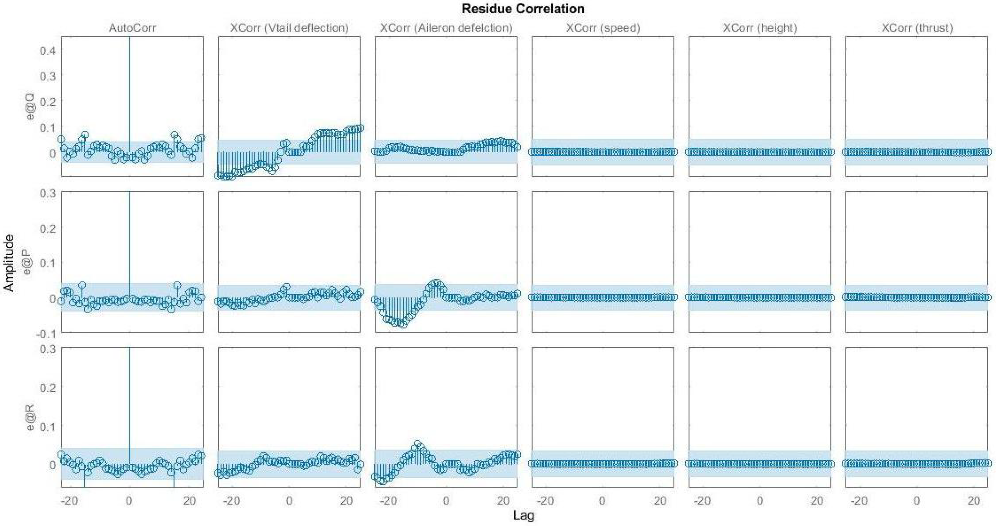
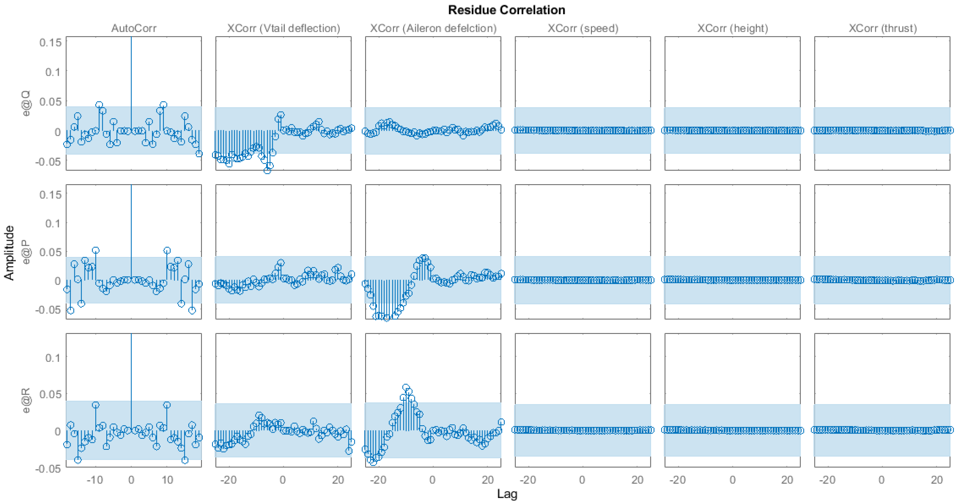
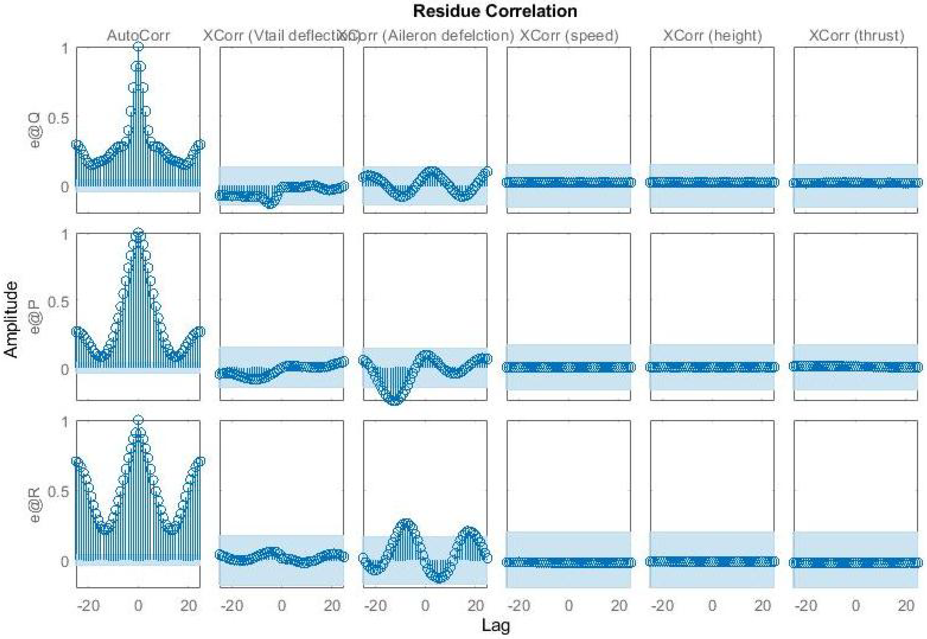
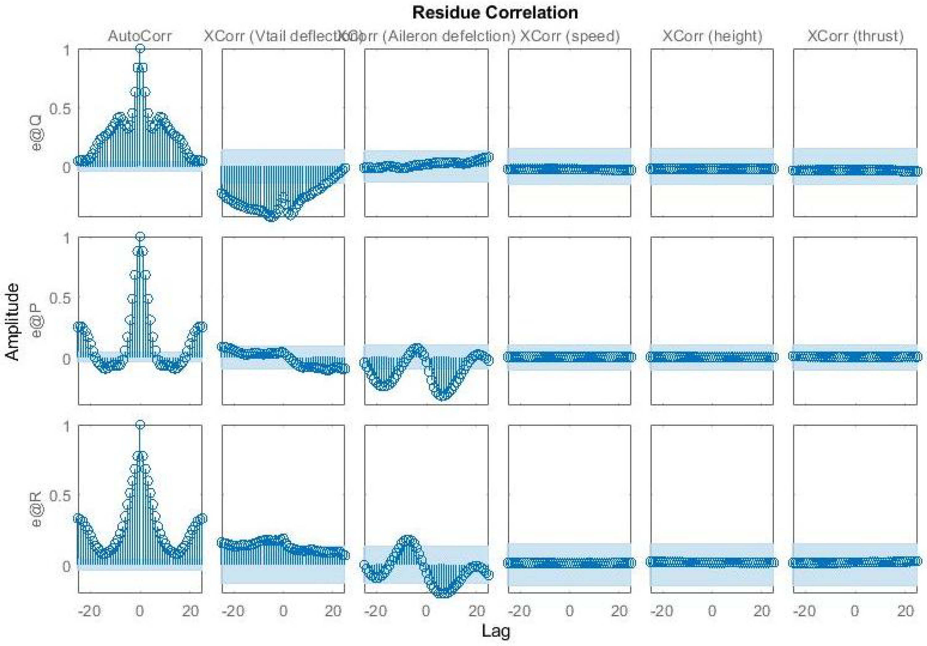
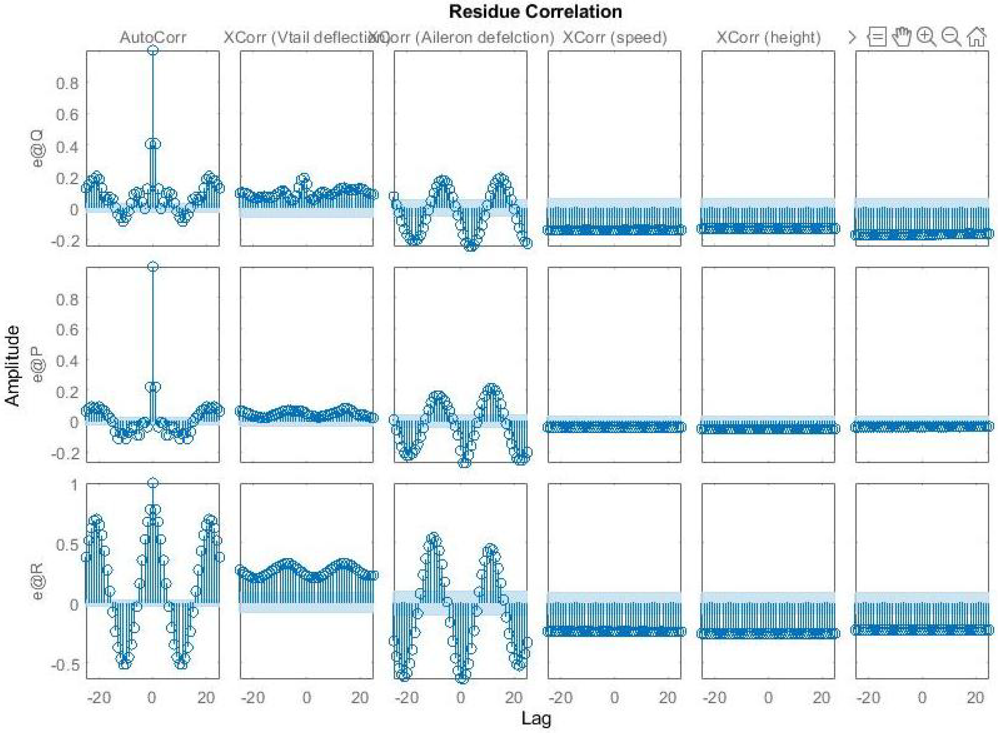
• Residual Analysis
• Percentage of fit to validation data
• Mean Squared Error (MSE)

The reader is also presented with a comparative analysis amongst the best model of each technique and final model is selected analysing the model quality using previously stated factors. This selected model is further validated to predict the outputs using a different data of the same flight regime.

4.1. Flight Designs

The first and foremost step of mathematical modelling of experimental UAV was data acquisition of inputs and outputs for an actual flight. A flight design was sorted out to cover all aspects of control surfaces under different flight conditions. Once, the flight design was finalized, flight was conducted and data was acquired for offline empirical mathematical modelling of the UAV. After modelling, a second flight was conducted to compare the predicted response using finalized model with actual flight response.

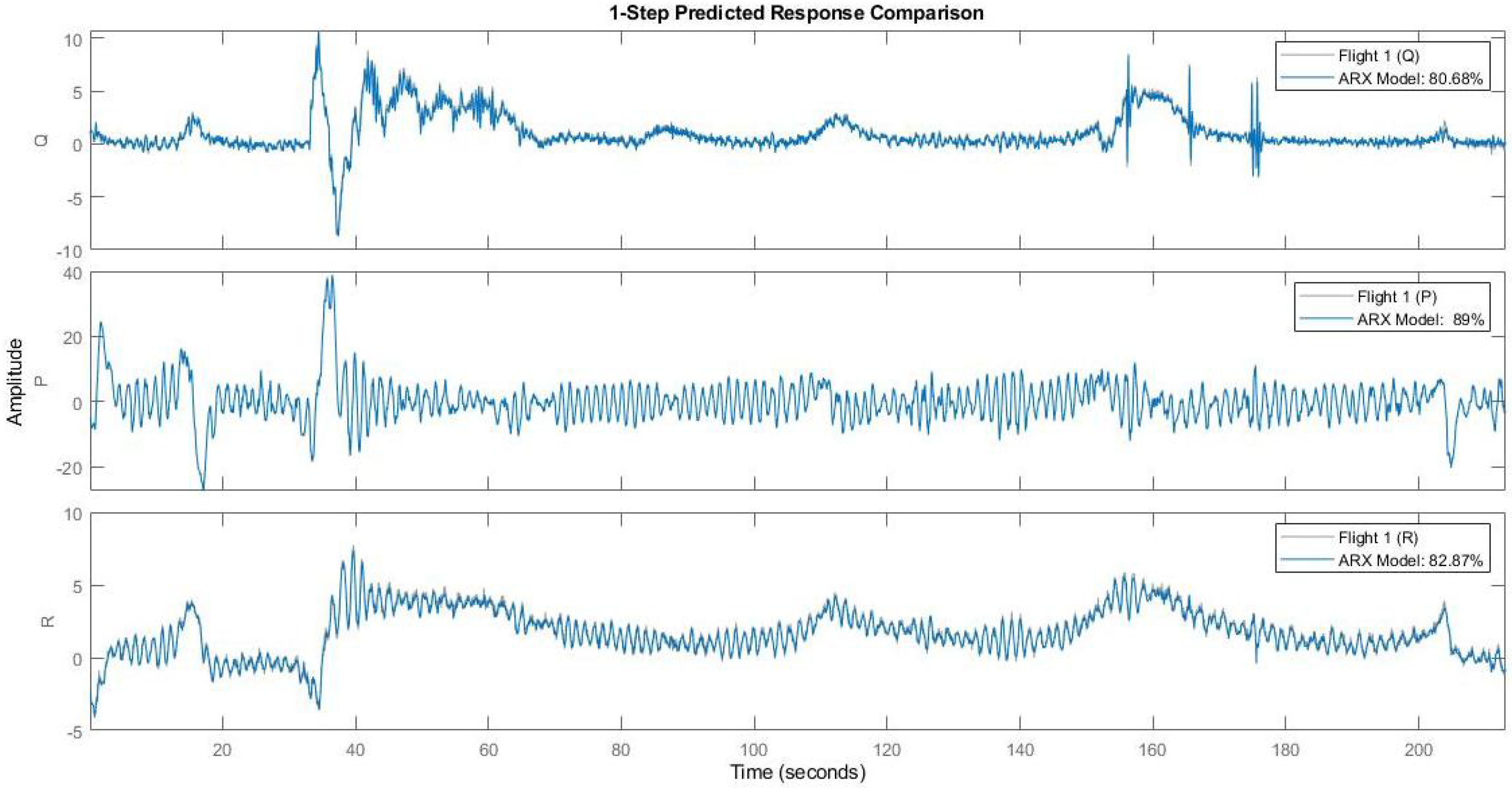
4.1.1. Flight 1 (Estimation)

The experimental UAV was given full throttle and held back with the catapult mechanism. The height profile along with x-axis acceleration and thrust shutoff point at time of parachute deployment of the UAV was used to identify the whole flight regime to be used for modelling. The UAV attains a certain height and then maintains that height while performing maneuvers to capture the complete range of control surface deflections for different flight conditions (Figure 1 and Figure 2).

After capturing the required data, it was trained offline to use it for system modelling. The data was divided in half. The first half comprising the takeoff and part of level flight was used for model estimations and the second half was used used for validation.

4.1.2. Flight 2 (Validation)

Finalizing the the mathematical model using flight 1 data led the authors to conduct validation trial. A second flight was conducted using the same flight design aspects discussed in Section 4.1.1. Different profiles for the validation sortie are shown in Figure 3, Figure 4, Figure 5, Figure 6, Figure 7 and Figure 8. Complete flight regime (takeoff till parachute deployment) was predicted using the mathematical model and the results are depicted in Section 4.9.

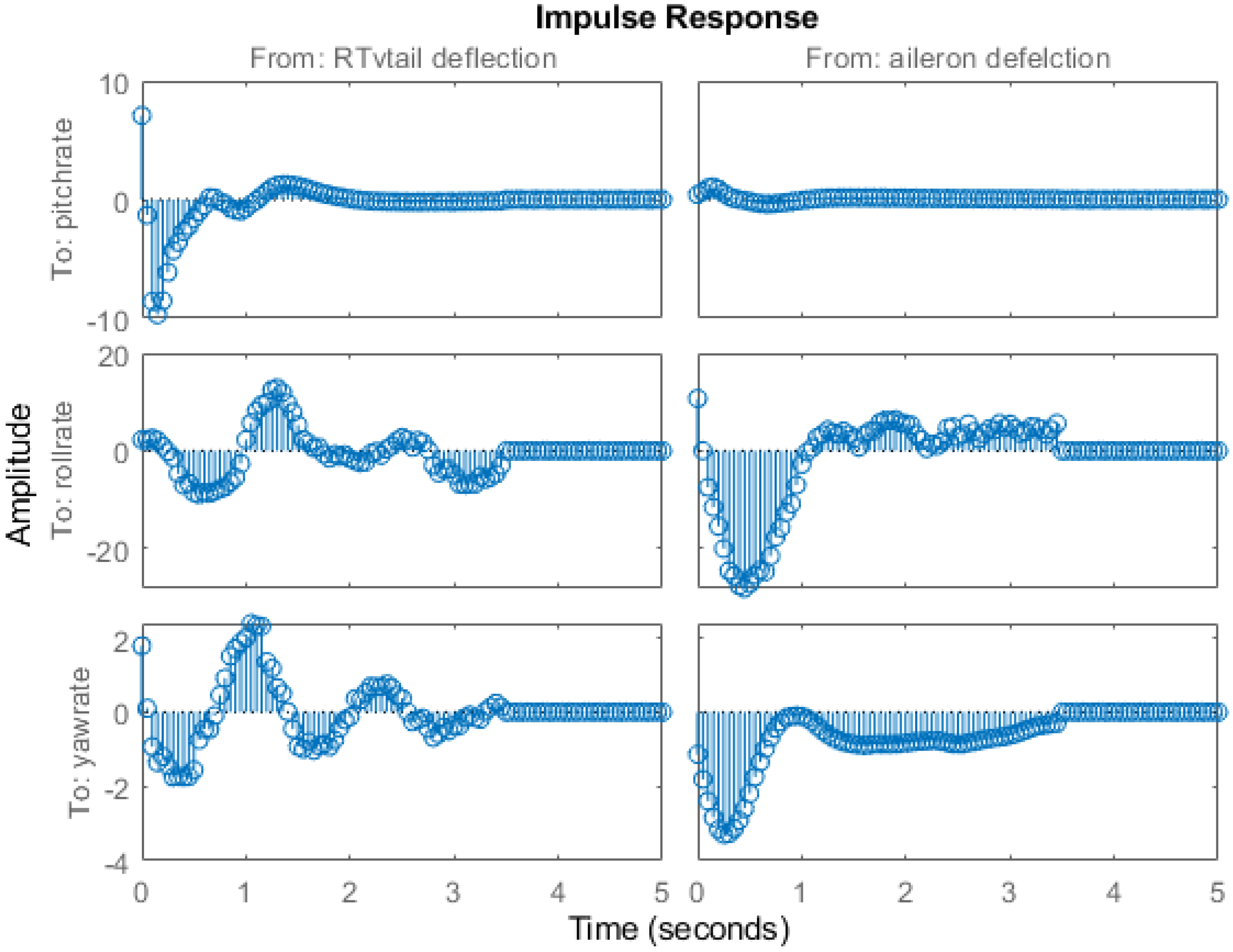
4.2. Finite Impulse Response (FIR) Model

From the FIR model response in Figure 9 the excitation orders for all the inputs are [50 50 50 50 50] and the time delay $T_s$ will be taken zero in further techniques. The FPE and MSE of FIR model is 3.352e+06 and 2.6e+04 respectively and fit percentage between modeled output and actual output is for pitch rate, roll rate and yaw rate is −1036%, 11.06%, −9067% respectively. The number of free coefficients of the impulse response model is 1050 which is quite high.

4.3. Auto Regressive Exogenous (ARX) Model

The model order for the ARX model was selected in an iterative fashion where different combinations of the order of polynomial $A\left(q\right)$ ($N_a$), order of polynomial $B\left(q\right)$ ($N_b$) were chosen. A total of 75 models were derived and training was performed on each of each model before a best ARX model with minimum FPE of 0.00257 and MSE of 0.6356 was finalized. Fit percentages to actual outputs are depicted in 1-step ahead prediction response of ARX model in Figure 10. The auto-correlation and cross-correlation plots of the model response (Figure 11) also shows that the selected model gives good confidence level as the residues are within the range the region marked blue which defines the part of the input response not been able to be predicted by the model. In our research we have set the confidence region to be 98%.

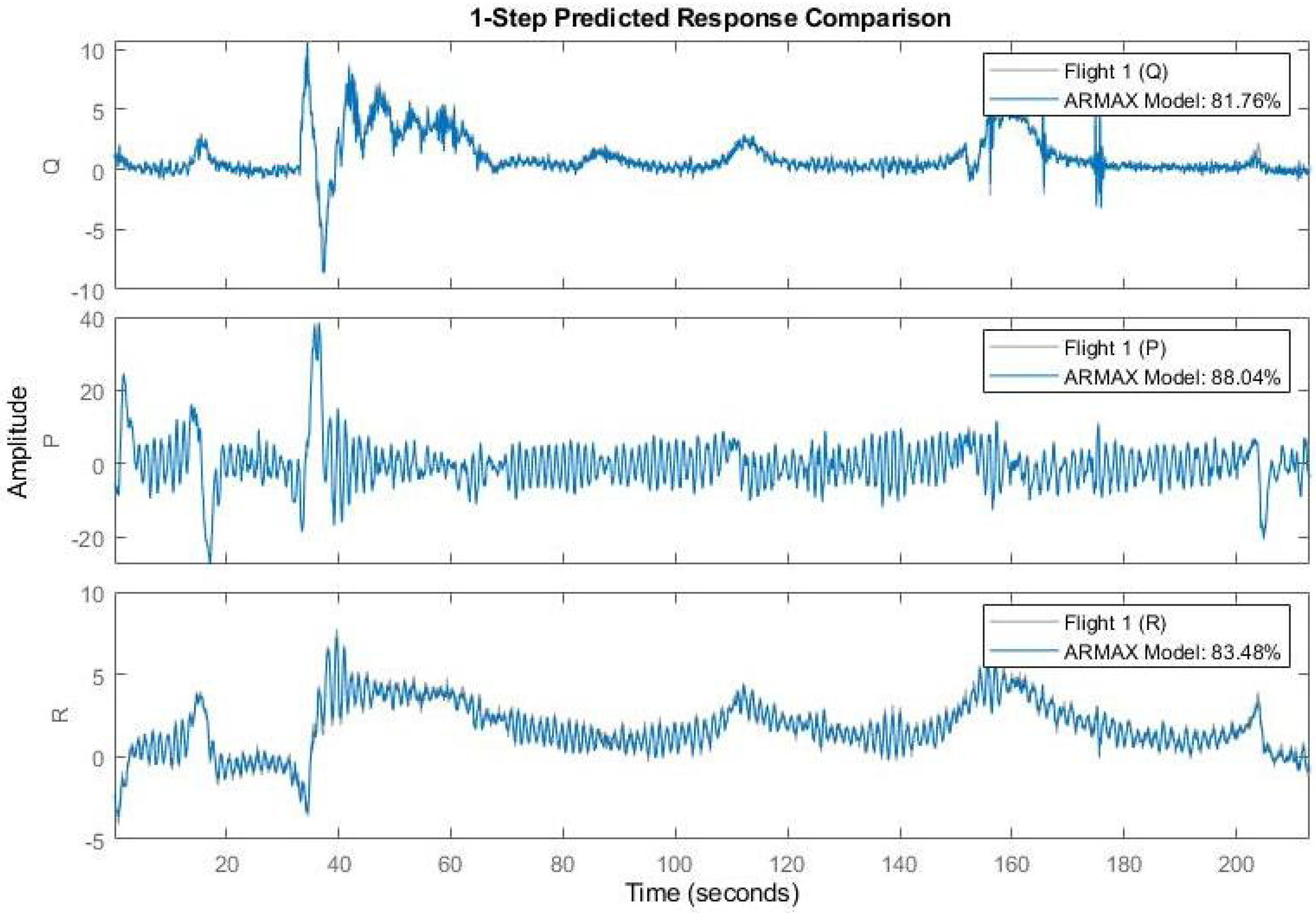
4.4. Autoregressive Moving Average eXogenous (ARMAX) Model

The same iterative approach was used for model order selection of ARMAX model. Final ARMAX model was selected after deriving and training a total of 125 model with FPE and MSE equal to 0.002208 and 0.6352. Fit percentages to actual outputs are depicted in 1-step ahead prediction response of ARX model in Figure 12. The auto-correlation and cross-correlation plots of the model response (Figure 13) also shows that the selected model gives good confidence level.

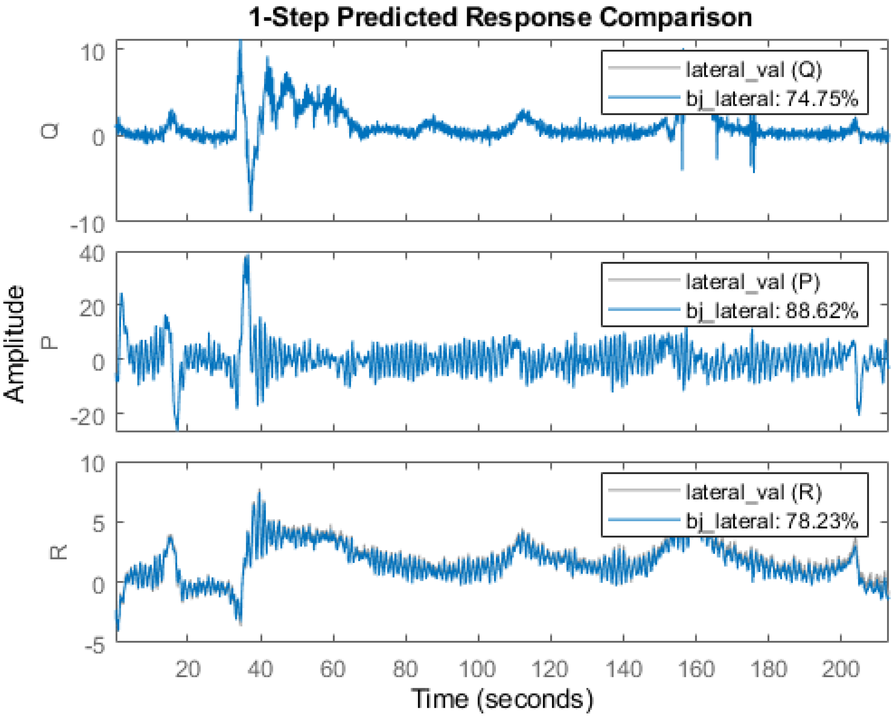
4.5. Box Jenkin’s (BJ Model)

Order selection procedure used in [44] was adopted to select the model order which gives satisfactory residue correlation (Figure 14) and fit percentages (Figure 15) along with an impressive FPE and MSE 0.005407 and 0.8946 respectively.

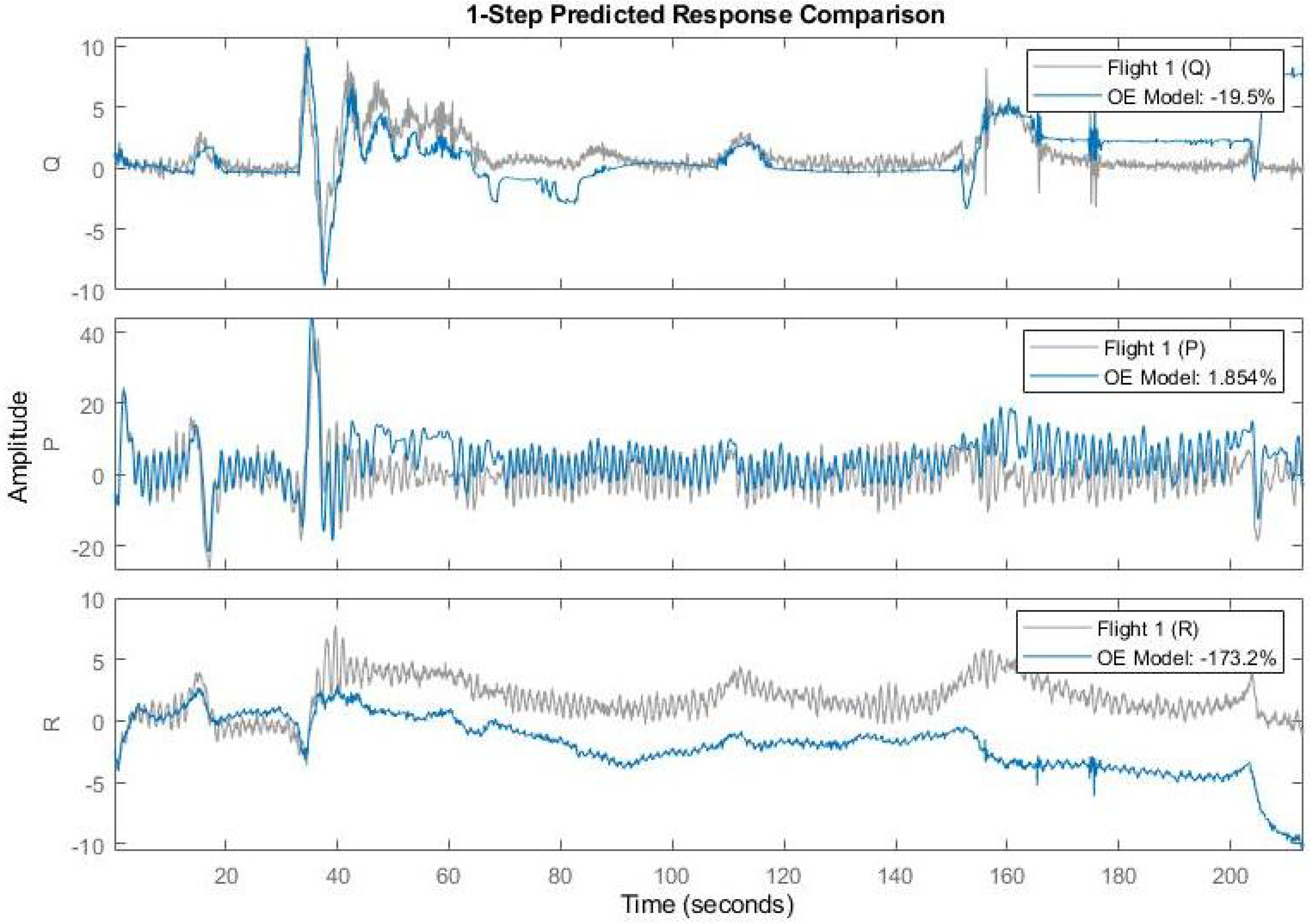
4.6. Output Error (OE) Model

The OE model response and residual correlation are shown in Figure 16 and Figure 17 respectively. As shown in the figure, the output error model is not able to predict the 1·step ahead predicted response. This can be attributed to the fact that output error model acts as a similation model in which the model response is computed using input data and initial conditions. Since no past outputs are being used to compute the response the error accumulates and the results deviate from actual response.

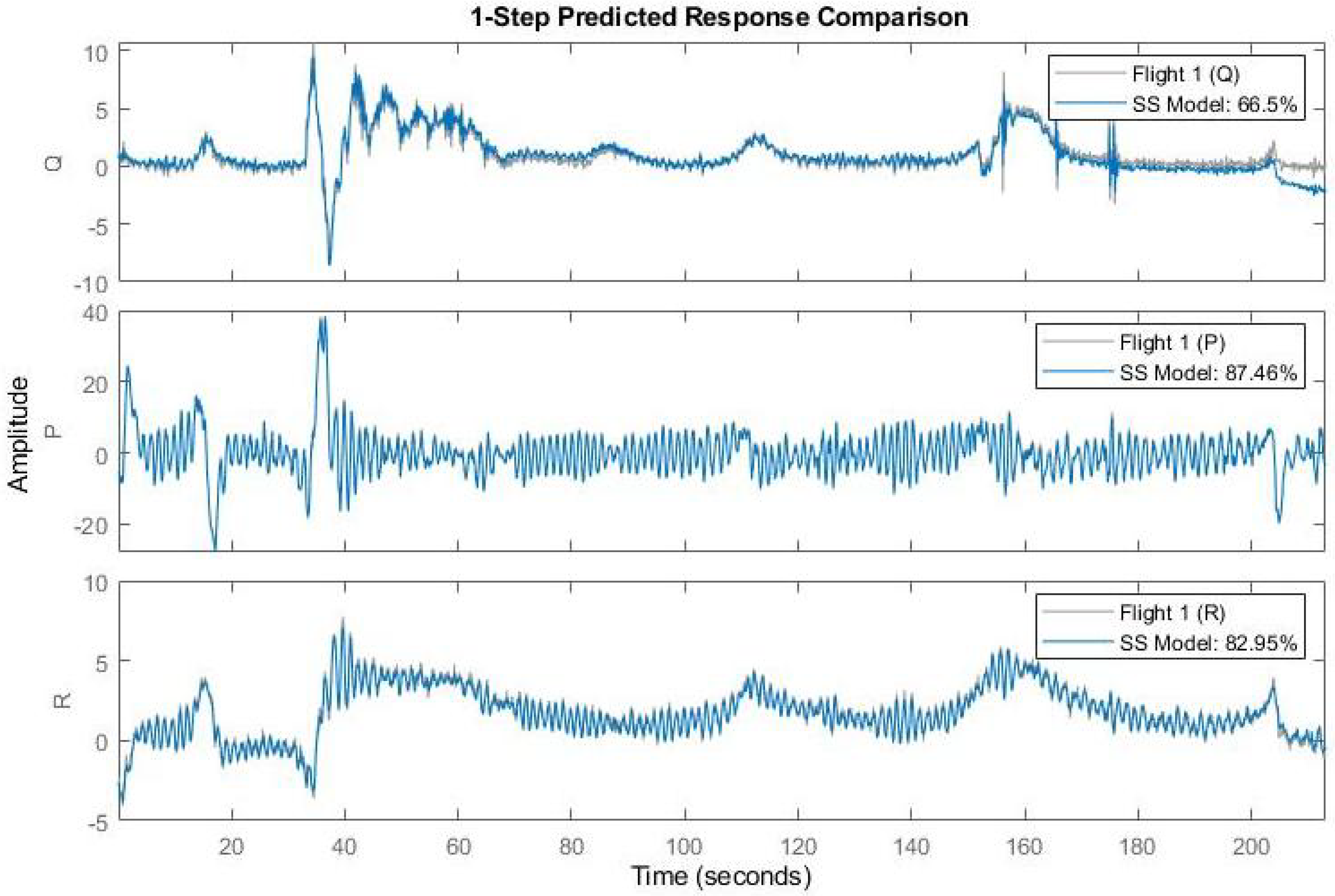
4.7. State Space Model

Figure 18 and Figure 19 shows the state space model fit percentages and residue correlation respectively. The model order is equal to 6 with FPE and MSE equal to 0.005307 and 0.7822 respectively. The lower model order of the state space model and the residual graphs of the same show that this model provides ease of computation by reducing the order without compromising the quality of the response.

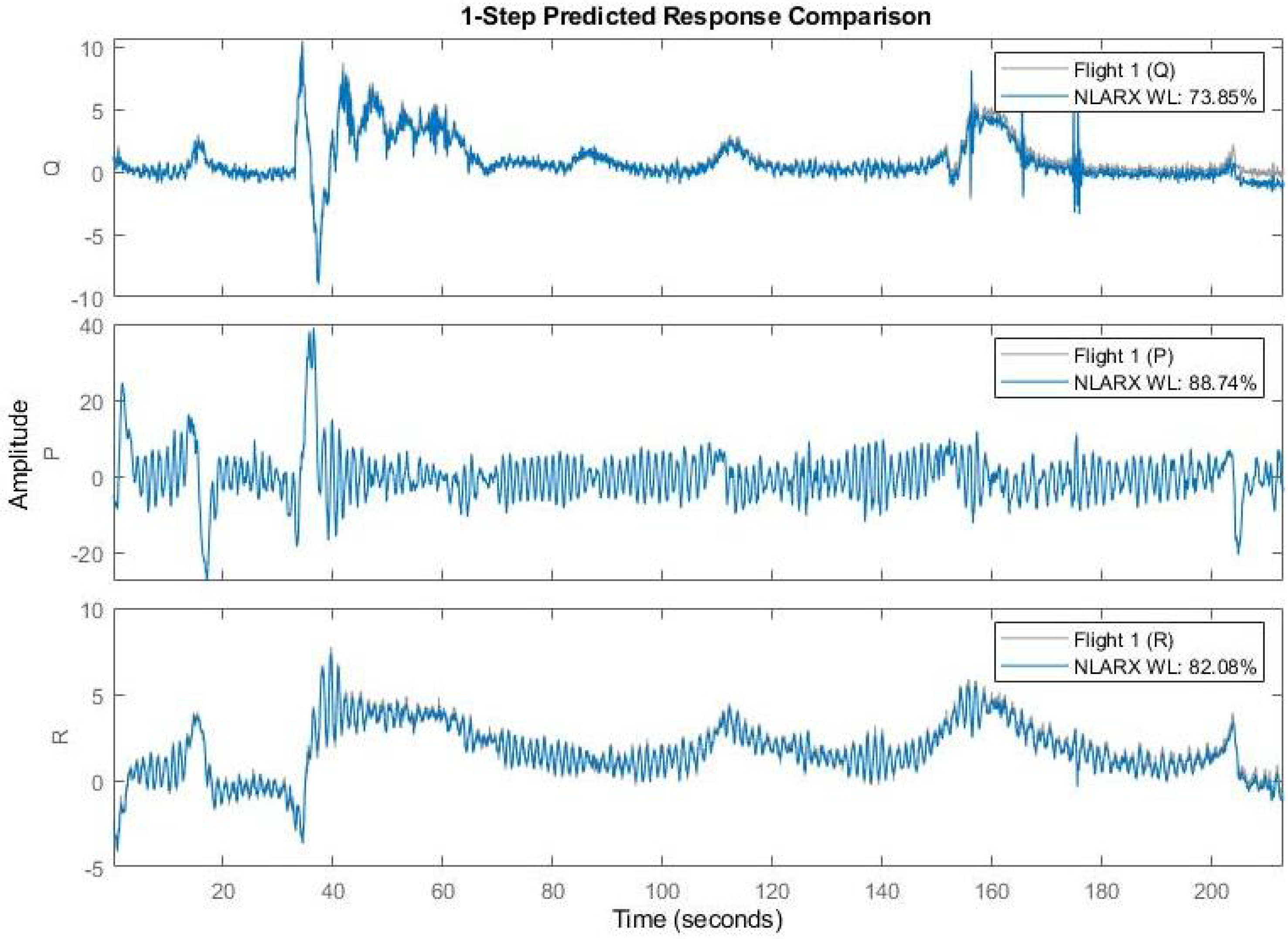
4.8. Non-Linear ARX Model

The fit percentages and residue correlation plots of non-linear ARX models with tree partition, wavelet network and neural network estimators are presented in Figure 20, Figure 21 and Figure 22. The Model order is selected to be the same as the best fit ARX model for further comparison. Although the results of wavelet network are acceptable but the added complexity in the model due to non linearity is not favored for time compressed computational environments. the same quality of model response is also provided by linear models.

4.9. Comparative Analysis

The comparison analysis of results for all linear and non-linear parametric model estimation techniques used in this research are tabulated in

Table 1. Comparison Analysis of Linear and Nonlinear Parametric Model Responses.

Parameter	ARX	ARMAX	BJ	OE	SS	NLARX
						TP	WL	NN
FPE	0.00257	0.0022	0.00868	2.611	0.0037	-	0.002688	-
MSE	0.6356	0.635	0.8518	16.29	0.74	3.998	0.643	0.6545
$PFit$	89%	88.04%	88.62%	1.854%	87.46%	63.16%	88.74%	87.7%
$QFit$	80.68%	81.76%	74.75%	−19.5%	66.5%	12.57%	73.85%	77.02%
$RFit$	82.87%	83.48%	78.23%	−173.2%	88.95%	−21.28%	82.08%	81.79%
Coeff.	210	135	72	105	102	-	-	-

for selection of best model based on parameters like model order, Final Prediction Error (FPE), Mean Square Error (MSE), fit percentages of roll rate (P), pitch rate(Q) and yaw rate (R), number of free parameters and perspective analysis of residue correlation.

ARMAX model and linear ARX model gave best values for FPE, MSE, fit percentages etc. Finally, ARMAX model was selected based on residue analysis. The next step was to validate the selected model on a different flight data covering the same flight regime. The comparison results for predicted output of ARMAX model and actual output data from validation sortie are presented in Figure 23 along with the residue correlation in Figure 24. The fit percentages of the ARMAX model are satisfactory and the residue correlation plot also shows good confidence level.

4.10. Discussion and Remarks

As evident from Table 1 the linear and non-linear parametric models give results which are acceptable for use in future design modifications and simulations of the UAV under test. However, the output error model can’t be used owing to the high deviations in predicted responses and measured responses. The reason for this can be attributed to the fact that the output error model takes only the previous inputs rather than the previous inputs and outputs for the prediction of the model response. The linear ARX model has higher model order as compared to the linear ARMAX model. However, The ARMAX model provides a better prediction with lower model order and hence, reducing the number of free coefficients in the model, which is usually desired.

Box Jenkins and state space model, although giving even lower model order and lesser number of coefficients in the model, The performance of these models based on fit percentages, mean squared error and final prediction error states render them of less utility in comparison to ARMAX and ARX models. The nonlinear ARX models with tree partition, wavelet network and neural network show acceptable fit percentages but the fact that the model is nonlinear, which adds to the complexity and computational time with high model orders, render them with less utilization. The last factor which has contributed towards the selection of best model amongst all model structures is the residual analysis. ARMAX model gives the best results on this model quality assessment parameter also. Hence, ARMAX model was selected as final model for verification of a different flight data.

4.11. Research Limitations

The research pertains to system identification utilizing various linear/nonlinear techniques. Limited research in this regard is available in literature to make it a benchmark for this research. The flights to be performed for the purpose of data gathering for model prediction clearly presents a financial and administrative challenge. The integrity of model prediction and its accuracy greatly enhances with availability of sufficient flight data. We believe that the technique presented in this research will present even more accurate results with the increase in the available flight data.

5. Conclusions

This paper describes the development of 6 DOF Flight Dynamics Model of the UAV followed by basic parameters of the UAV under test and launch and recovery mechanism of the same. System identification was applied to actual flight data, and various linear and nonlinear parametric models with different model structures were developed. The model structures included the impulse response model, ARX, ARMAX, Box Jenkin’s, Output Error, State Space, Nonlinear ARX models with tree partition, wavelet network, and neural network models. Several models were developed for each model structure, and each model was trained before the selection of the final model from that category. A comprehensive analysis was carried out for all the models, and after detailed comparison and analysis best fit model was finalized to be ARMAX model, which has FPE of 0.0022. The model was further used to predict output of a different sortie with same flight regime and the fit percentages of the modeled output to actual output of Roll rate (P) was 88.72%, Pitch Rate (Q) was 72.81% and Yaw Rate (R) was 38.36% which is quite satisfactory. It is imperative to highlight that the proposed framework presented in this study provides a consolidated platform which can be utilized by researchers to perform model estimation for any similar platform. The best fit model structure most suitable for that particular configuration can be selected accordingly as per the proposed benchmarks. The research presented in this paper is purely original and to the best of author’s knowledge, such a detailed analysis is presented for the first time in literature.

References

- Gul, F.; Mir, I.; Abualigah, L.; Mir, S.; Altalhi, M. Cooperative multi-function approach: A new strategy for autonomous ground robotics. Future Gener. Comput. Syst. 2022, 134, 361–373. [Google Scholar] [CrossRef]
- Din, A.F.U.; Mir, I.; Gul, F.; Nasar, A.; Rustom, M.; Abualigah, L. Reinforced Learning-Based Robust Control Design for Unmanned Aerial Vehicle. Arab. J. Sci. Eng. 2022, 1–16. [Google Scholar] [CrossRef]
- Din, A.F.U.; Akhtar, S.; Maqsood, A.; Habib, M.; Mir, I. Modified model free dynamic programming: An augmented approach for unmanned aerial vehicle. Appl. Intell. 2022, 1–21. [Google Scholar] [CrossRef]
- Mir, I.; Eisa, S.A.; Maqsood, A. Review of dynamic soaring: Technical aspects, nonlinear modeling perspectives and future directions. Nonlinear Dyn. 2018, 94, 3117–3144. [Google Scholar] [CrossRef]
- Mir, I.; Maqsood, A.; Akhtar, S. Biologically inspired dynamic soaring maneuvers for an unmanned air vehicle capable of sweep morphing. Int. J. Aeronaut. Space Sci. 2018, 19, 1006–1016. [Google Scholar] [CrossRef]
- Mir, I.; Maqsood, A.; Akhtar, S. Dynamic modeling & stability analysis of a generic UAV in glide phase. In Proceedings of the MATEC Web of Conferences, EDP Sciences, Ulis, France, 10 July 2017; Volume 114, p. 01007. [Google Scholar]
- Mir, I.; Eisa, S.A.; Taha, H.; Maqsood, A.; Akhtar, S.; Islam, T.U. A stability perspective of bioinspired unmanned aerial vehicles performing optimal dynamic soaring. Bioinspiration Biomim. 2021, 16, 066010. [Google Scholar] [CrossRef]
- Gul, F.; Mir, S.; Mir, I. Coordinated Multi-Robot Exploration: Hybrid Stochastic Optimization Approach. In Proceedings of the AIAA SCITECH 2022 Forum, San Diego, CA, USA, 3–7 January 2022; p. 1414. [Google Scholar]
- Gul, F.; Mir, S.; Mir, I. Multi Robot Space Exploration: A Modified Frequency Whale Optimization Approach. In Proceedings of the AIAA SCITECH 2022 Forum, San Diego, CA, USA, 3–7 January 2022; p. 1416. [Google Scholar]
- Gul, F.; Mir, I.; Abualigah, L.; Sumari, P. Multi-Robot Space Exploration: An Augmented Arithmetic Approach. IEEE Access 2021, 9, 107738–107750. [Google Scholar] [CrossRef]
- Gul, F.; Rahiman, W.; Alhady, S.N.; Ali, A.; Mir, I.; Jalil, A. Meta-heuristic approach for solving multi-objective path planning for autonomous guided robot using PSO–GWO optimization algorithm with evolutionary programming. J. Ambient Intell. Humaniz. Comput. 2021, 12, 7873–7890. [Google Scholar] [CrossRef]
- Gul, F.; Mir, I.; Rahiman, W.; Islam, T.U. Novel Implementation of Multi-Robot Space Exploration Utilizing Coordinated Multi-Robot Exploration and Frequency Modified Whale Optimization Algorithm. IEEE Access 2021, 9, 22774–22787. [Google Scholar] [CrossRef]
- Gul, F.; Mir, I.; Abualigah, L.; Sumari, P.; Forestiero, A. A Consolidated Review of Path Planning and Optimization Techniques: Technical Perspectives and Future Directions. Electronics 2021, 10, 2250. [Google Scholar] [CrossRef]
- Gul, F.; Alhady, S.S.N.; Rahiman, W. A review of controller approach for autonomous guided vehicle system. Indones. J. Electr. Eng. Comput. Sci. 2020, 20, 552–562. [Google Scholar] [CrossRef]
- Gul, F.; Rahiman, W. An Integrated approach for Path Planning for Mobile Robot Using Bi-RRT. In Proceedings of the IOP Conference Series: Materials Science and Engineering, Kuala Terengganu, Malaysia, 27–28 August 2019; IOP Publishing: Kuala Terengganu, Malaysia, 2019; Volume 697, p. 012022. [Google Scholar]
- Gul, F.; Rahiman, W.; Nazli Alhady, S.S. A comprehensive study for robot navigation techniques. Cogent Eng. 2019, 6, 1632046. [Google Scholar] [CrossRef]
- Szczepanski, R.; Tarczewski, T.; Grzesiak, L.M. Adaptive state feedback speed controller for PMSM based on Artificial Bee Colony algorithm. Appl. Soft Comput. 2019, 83, 105644. [Google Scholar] [CrossRef]
- Szczepanski, R.; Bereit, A.; Tarczewski, T. Efficient Local Path Planning Algorithm Using Artificial Potential Field Supported by Augmented Reality. Energies 2021, 14, 6642. [Google Scholar] [CrossRef]
- Szczepanski, R.; Tarczewski, T. Global path planning for mobile robot based on Artificial Bee Colony and Dijkstra’s algorithms. In Proceedings of the 2021 IEEE 19th International Power Electronics and Motion Control Conference (PEMC), Gliwice, Poland, 25–29 April 2021; pp. 724–730. [Google Scholar]
- Khalil, B.; Yesildirek, A. System identification of UAV under an autopilot trajectory using ARX and Hammerstein-Wiener methods. In Proceedings of the 7th International Symposium on Mechatronics and Its Applications, Sharjah, United Arab Emirates, 20–22 April 2010; pp. 1–5. [Google Scholar]
- Mir, I.; Akhtar, S.; Eisa, S.; Maqsood, A. Guidance and control of standoff air-to-surface carrier vehicle. Aeronaut. J. 2019, 123, 283–309. [Google Scholar] [CrossRef]
- Mir, I.; Taha, H.; Eisa, S.A.; Maqsood, A. A controllability perspective of dynamic soaring. Nonlinear Dyn. 2018, 94, 2347–2362. [Google Scholar] [CrossRef]
- Mir, I.; Maqsood, A.; Eisa, S.A.; Taha, H.; Akhtar, S. Optimal morphing–augmented dynamic soaring maneuvers for unmanned air vehicle capable of span and sweep morphologies. Aerosp. Sci. Technol. 2018, 79, 17–36. [Google Scholar] [CrossRef]
- Mir, I.; Maqsood, A.; Taha, H.E.; Eisa, S.A. Soaring Energetics for a Nature Inspired Unmanned Aerial Vehicle. In Proceedings of the AIAA Scitech 2019 Forum, San Diego, CA, USA, 7–11 January 2019; p. 1622. [Google Scholar]
- Hussain, A.; Hussain, I.; Mir, I.; Afzal, W.; Anjum, U.; Channa, B.A. Target Parameter Estimation in Reduced Dimension STAP for Airborne Phased Array Radar. In Proceedings of the 2020 IEEE 23rd International Multitopic Conference (INMIC), Bahawalpur, Pakistan, 5–7 November 2020; pp. 1–6. [Google Scholar]
- Hussain, A.; Anjum, U.; Channa, B.A.; Afzal, W.; Hussain, I.; Mir, I. Displaced Phase Center Antenna Processing For Airborne Phased Array Radar. In Proceedings of the 2021 International Bhurban Conference on Applied Sciences and Technologies (IBCAST), Islamabad, Pakistan, 12–16 January 2021; pp. 988–992. [Google Scholar]
- Gul, F.; Rahiman, W. Mathematical Modeling of Self Balancing Robot and Hardware Implementation. In Proceedings of the 11th International Conference on Robotics, Vision, Signal Processing and Power Applications: Universiti Sains Malaysia, Penang, Malaysia, 5–6 April 2021; Springer: Penang, Malaysia, 2022; pp. 20–26. [Google Scholar]
- Hopping, B.M.; Garrett, T.M. Low Speed Airfoil Design for Aerodynamic Improved Performance of UAVs. U.S. Patent 9,868,525, 29 June 2018. [Google Scholar]
- Mir, I.; Maqsood, A.; Akhtar, S. Optimization of dynamic soaring maneuvers to enhance endurance of a versatile UAV. In Proceedings of the IOP Conference Series: Materials Science and Engineering; IOP Publishing: Bangkok, Thailand, 2017; Volume 211, p. 012010. [Google Scholar]
- Mestrinho, J.; Gamboa, P.; Santos, P. Design optimization of a variable-span morphing wing for a small UAV. In Proceedings of the 52nd AIAA/ASME/ASCE/AHS/ASC Structures, Structural Dynamics and Materials Conference, Denver, CO, USA, 4–7 April 2011; Volume 47. [Google Scholar]
- Mir, I.; Eisa, S.A.; Taha, H.; Maqsood, A.; Akhtar, S.; Islam, T.U. A stability perspective of bio-inspired UAVs performing dynamic soaring optimally. Bioinspir. Biomim. 2021. [Google Scholar] [CrossRef]
- Ahsan, J.; Ahsan, M.; Jamil, A.; Ali, A. Grey Box Modeling of Lateral-Directional Dynamics of a UAV through System Identification. In Proceedings of the 2016 International Conference on Frontiers of Information Technology (FIT), Islamabad, Pakistan, 19–21 December 2016; pp. 324–329. [Google Scholar]
- Rasheed, A. Grey box identification approach for longitudinal and lateral dynamics of UAV. In Proceedings of the 2017 International Conference on Open Source Systems & Technologies (ICOSST), Lahore, Pakistan, 18–20 December 2017; pp. 10–14. [Google Scholar]
- BELGE, E.; Hızır, K.; PARLAK, A.; ALTAN, A.; HACIOĞLU, R. Estimation of small unmanned aerial vehicle lateral dynamic model with system identification approaches. Balk. J. Electr. Comput. Eng. 2020, 8, 121–126. [Google Scholar] [CrossRef]
- Altan, A.; Aslan, Ö.; Hacıoğlu, R. Model predictive control of load transporting system on unmanned aerial vehicle (UAV). In Proceedings of the Fifth International Conference on Advances in Mechanical and Robotics Engineering, Rome, Italy, 1 May 2017; Institute of Research Engineers and Doctors: Rome, Italy, 2017; pp. 1–4. [Google Scholar]
- Dube, C.; Pedro, J.O. Modelling and closed-loop system identification of a quadrotor-based aerial manipulator. J. Phy. Conf. Ser. 2018, 1016, 012007. [Google Scholar]
- Cavanini, L.; Ferracuti, F.; Longhi, S.; Monteriù, A. Ls-svm for lpv-arx identification: Efficient online update by low-rank matrix approximation. In Proceedings of the 2020 International Conference on Unmanned Aircraft Systems (ICUAS), Athens, Greece, 1–4 September 2020; pp. 1590–1595. [Google Scholar]
- Cavanini, L.; Ippoliti, G.; Camacho, E.F. Model predictive control for a linear parameter varying model of an UAV. J. Intell. Robot. Syst. 2021, 101, 1–18. [Google Scholar]
- Belge, E.; Altan, A.; Hacıoğlu, R. Metaheuristic Optimization-Based Path Planning and Tracking of Quadcopter for Payload Hold-Release Mission. Electronics 2022, 11, 1208. [Google Scholar] [CrossRef]
- Weng, Y.; Nan, D.; Wang, N.; Liu, Z.; Guan, Z. Compound robust tracking control of disturbed quadrotor unmanned aerial vehicles: A data-driven cascade control approach. Trans. Inst. Meas. Control 2022, 44, 941–951. [Google Scholar] [CrossRef]
- Lecerf, M.; Allaire, D.; Willcox, K. Methodology for dynamic data-driven online flight capability estimation. AIAA J. 2015, 53, 3073–3087. [Google Scholar] [CrossRef]
- Yu, Y.; Guo, J.; Ahn, C.K.; Xiang, Z. Neural adaptive distributed formation control of nonlinear multi-uavs with unmodeled dynamics. IEEE Trans. Neural Netw. Learn. Syst. 2022. [Google Scholar] [CrossRef]
- Saengphet, W.; Tantrairatn, S.; Thumtae, C.; Srisertpol, J. Implementation of system identification and flight control system for UAV. In Proceedings of the 2017 3rd International Conference on Control, Automation and Robotics (ICCAR), Nagoya, Japan, 24–26 April 2017; pp. 678–683. [Google Scholar]
- Bnhamdoon, O.A.A.; Mohamad Hanif, N.H.H.; Akmeliawati, R. Identification of a quadcopter autopilot system via Box–Jenkins structure. Int. J. Dyn. Control 2020, 8, 835–850. [Google Scholar] [CrossRef]
- Ayyad, A.; Chehadeh, M.; Awad, M.I.; Zweiri, Y. Real-time system identification using deep learning for linear processes with application to unmanned aerial vehicles. IEEE Access 2020, 8, 122539–122553. [Google Scholar] [CrossRef]
- Munguía, R.; Urzua, S.; Grau, A. EKF-based parameter identification of multi-rotor unmanned aerial vehiclesmodels. Sensors 2019, 19, 4174. [Google Scholar] [CrossRef]
- Puttige, V.R.; Anavatti, S.G. Real-time system identification of unmanned aerial vehicles: A multi-network approach. J. Comput. 2008, 3, 31–38. [Google Scholar] [CrossRef]
- Wu, Z.; Karimi, H.R.; Dang, C. An approximation algorithm for graph partitioning via deterministic annealing neural network. Neural Netw. 2019, 117, 191–200. [Google Scholar] [CrossRef]
- Hoffer, N.V.; Coopmans, C.; Jensen, A.M.; Chen, Y. A survey and categorization of small low-cost unmanned aerial vehicle system identification. J. Intell. Robot. Syst. 2014, 74, 129–145. [Google Scholar] [CrossRef]
- Sierra, J.E.; Santos, M. Modelling engineering systems using analytical and neural techniques: Hybridization. Neurocomputing 2018, 271, 70–83. [Google Scholar] [CrossRef]
- Stevens, B.L.; Lewis, F.L.; Johnson, E.N. Aircraft Control and Simulation: Dynamics, Controls Design, and Autonomous Systems; John Wiley & Sons: Hoboken, NJ, USA, 2015. [Google Scholar]