
Experimental Characterization Techniques for Solid-Liquid Slurry Flows in Pipelines: A Review


Department of Chemical Engineering, CIEPQPF, University of Coimbra, 3030-790 Coimbra, Portugal
Processes 2022, 10(3), 597; https://doi.org/10.3390/pr10030597
Submission received: 14 February 2022
/
Revised: 8 March 2022
/
Accepted: 15 March 2022
/
Published: 18 March 2022
(This article belongs to the Section Process Control and Monitoring)
Abstract
:In industrial environments, having instrumentation able to attain fast, accurate, and autonomous measurements is pivotal to understanding the dynamics of liquid and particles during transport. Ideally, these instruments, consisting of either probes or sensors, should be robust, fast, and unintrusive, i.e., not cause interference on the very flows being monitored, and require minimal maintenance. Beyond monitoring, the process knowledge gained through real time inspection allows teams to make informed technical decisions based on particle behavior, i.e., settling of particles causing pipe wear and clustering or blockages that can damage the unit or cause shutdowns, both of which with economical drawbacks. The purpose of this review is to examine experimental measurement techniques used to characterize physical properties and operational parameters of solid-liquid slurry flows, focusing on non-ionizing radiation methods. With this text the intent is not to provide an exhaustive examination of each individual technique but rather an overview on the most pertinent types of instrumentation, which will be presented, in addition to application examples from the literature, while directing the reader for pertinent seminal and review papers for a more in-depth analysis.
1. Introduction
1.1. Historical Importance of Solid-Liquid Flows
Flows involving a mixture of suspended solid particles in a flowing fluid have been extensively used by different civilizations through time, most notably the Egyptian, Roman, and Greek empires, but the earliest record from an engineering application of solid-liquid suspension flow was in 1860 in the Suez Canal, in Egypt [1].
Nowadays, the transport of solids suspended in liquids using pipelines has become ubiquitous in traditional industrial fields such as chemical, foodstuffs and pharmaceuticals production, mineral and construction materials transportation (such as coal, iron ore, sand, crushed rock, cement, and even wet concrete to name a few examples), waste treatment, both municipal and industrial, and emerging industries dealing with “intelligent” materials and biological systems [2,3,4]. Hundreds of other products in various fields also use this type of transport, including radioactive materials, grains, and hospital supplies.
In industrial environments having instrumentation able to attain fast, accurate, and autonomous measurements is pivotal to understanding the dynamics of liquid and particles during transport. Ideally, these instruments, consisting of either probes or sensors, should be robust, fast, and unintrusive, i.e., not cause interference on the very flows being monitored, and require minimal maintenance. Beyond monitoring, the process knowledge gained through real time inspection allows technical teams to make informed decisions based on particle behavior, i.e., settling of particles causing pipe wear, clustering, or blockages that can damage the unit or cause shutdowns, both of which have economic drawbacks [5].
1.2. Classification of Solid-Liquid Suspension Flows
The flow of solids suspended in liquids, solid-liquid suspensions, sometimes referred to as slurry flow for higher particle concentrations, are a subclass of multiphase flows. These flows are characterized by a wide range of different particle sizes, from nanometers to millimeters, concentrations and having diverse densities. If the densities of the liquid and solid particles differ significantly then settling will occur and these are called settling suspensions. These flows can be Newtonian or non-Newtonian; however, in this review we are only concerned with the Newtonian behavior.
Suspensions or slurries containing medium or coarser particles with density higher than the density of the liquid tend to settle and accumulate at the bottom of the vessel or pipe, resulting in different flow regimes affected by particle concentration and flow velocity [4]. Settling slurries or suspensions exhibit different flow regimes or flow patterns which are defined by visual inspection of the solid or dispersed phase.
The flow regime is intrinsically linked with the relation between flow velocity and particles characteristics such as particle size and density. It affects the pressure drop magnitude, pipe erosion or wear, and other performance characteristics. The complex nature of slurry flows and transitions between flow regimes hinders a perfect classification of the regimes or patterns. The first classification of solid-liquid suspensions in horizontal pipelines was based on the Reynolds Number (Re) and average particle size established by Durand and Condolios in 1952 for particles with a specific gravity of 2.65, and it was as follows [2,6]:
- For particles smaller than 40 μm an homogeneous suspension is assumed.
- For particle sizes from 40 μm to 0.15 mm the suspensions are maintained by turbulence.
- For particle sizes between 0.15 mm and 1.5 mm a suspension with saltation is considered.
- For particles greater than 1.5 mm a regime of saltation is dominant.
This classification was refined throughout the years by several researchers, including Govier & Aziz who brought forward the following classification for fine and coarse particles [1,6]:
- Ultrafine particles: particle size smaller than 10 μm where gravitational forces are negligible.
- Fine particles: particle sizes between 10 μm and 100 μm, carried fully suspended although subject to concentration gradients and gravitational forces.
- Medium sized particles: from 100 μm until 1000 μm particles move with a deposit at the bottom of the pipe and with a vertical concentration gradient.
- Coarse particles: particles sizes ranging from 1000 μm until 10,000 μm. These are seldom fully suspended and form deposits on the bottom of the pipe.
- Ultra-coarse particles are larger than 10 mm. These particles are transported as a moving bed on the bottom of the pipe.
Since Govier & Aziz did not account for particle density in their work, the above specified ranges serve only as guidelines and will shift according to density variations.
Overall, in the literature, and also in this review, the following classification introduced by Wilson et al. (1992) for slurry flows regimes is used [7] (Figure 1):
- Pseudo-homogenous regime, typical of flows laden with fine particles (typically fine sand of particle sizes between 60 and 200 micron) flowing at high velocity.
- Heterogeneous flow for which both inter-granular contact and fluid support mechanisms are significant.
- Fully stratified regime, typical of flow conveying large, rapidly settling particles at low velocity.
The pseudo-homogenous regime (Figure 1a) is characteristic of flows with fine particles (typically fine sand of particle sizes ranging from 60 and 200 micron) flowing at high velocity. The distribution of suspended particles is close to uniform although some gradient usually occurs in the pipe cross section (Figure 1a), which is due to the particle weight being carried by phenomena associated with fluid turbulence, and flow energy loss is caused by viscous friction; on the opposite side of the spectra lies the fully stratified flow regime (Figure 1c) which is typical for large, rapidly settling particles at low velocity. Settling occurs as a consequence of their submerged weight, which cannot be carried by flow turbulence, travelling in the lower part of the pipe cross-section by saltation or as a sliding bed (Figure 1c). Particle contacts with each other and with a pipe wall greatly contribute to the overall flow friction; in-between these two opposites flow regimes an intermediate case (Figure 1b) can be identified, the heterogeneous flow, for which both inter-granular contact and fluid support mechanisms are substantial (Figure 1b). In this regime, for relatively large particles, the heterogeneous flow regime is more stratified with a detectable sliding bed and particle transportation occurring either by turbulent eddies or by mutual collisions above the sliding bed. Also, flows of broadly graded particles in a Newtonian fluid carrier are frequently encountered in practical applications in which particles of quite different sizes are supported by different mechanisms interacting with each other.
Although beyond the scope of this review paper, and in addition to the aforementioned flow regimes, a case specific slurry flow regime in microreactors has also been documented in the literature: slurry Taylor flow or segmented slurry flow. In these types of flow regimes, the slurry flow is segmented by gas bubbles (Figure 2). These complex slurry flows have been gaining increasingly interest due to the potential wide range of applications in chemical/chemistry processes [9,10].
1.3. Solid-Liquid Flow Properties and Process Parameters: Characterization Techniques
The first systematic characterization of a solid-water mixture flow was performed in 1906 by Nora Blatch using a 25 mm (1 in) diameter horizontal pipe. In her studies pressure drops were accounted as a function of flow, density, and solids concentration [1,3].
The ability to characterize and monitor solid-liquid suspensions flows is of paramount importance in several industries. Having a comprehensive on-line control strategy for data acquisition is paramount in the production of high-quality products, uneventful plant operation, and cost-effective management of wastes and resources as well in continuous design improvement of flow and pumping equipment. In theory, this control strategy seems to be a deceptively straightforward application, but the practical implementation is, nevertheless, quite complex [5]. Conventionally, this implementation consisted of a limited number of discrete sensors distributed throughout plant, in points identified as critically important, and this sums up the usual course of action when monitoring and/or controlling the plant operation. A drawback from this oversimplified solution is an invariable loss of key information of both physical and chemical processes occurs in the manufacturing process.
For slurry conveying in a piping system, in addition to the known geometrical properties, characterization of slurry flows focuses on the measurement and monitoring of local and global particle and flow properties [5,11]:
Geometrical Properties
1. Pipe diameter, 2. Pipe roughness, and 3. Pipe inclination—coupled with particle size and shape these geometric characteristics have a significant impact on friction losses and deposition velocity of settling slurries and are defined during the rig design taking into account the nature of the slurry being conveyed.
Particle Properties
4. Particle density/material, 5. Particle size distribution, and 6. Particle shape—accurate characterization of particle properties enables process understanding and safeguards from particle settling and pipe erosion.
Local Flow Properties
7. Particle and slurry velocity—determines if the system is operating as designed for the slurry to avoid particle settling which results in pipe erosion or blockage. Average velocities can be determined through the use of multiple sensors and cross-correlation of signal fluctuations. Point velocities can also be measured.
8. In-situ and delivered solids/particle concentration for each phase—weight and volume percent—to determine if the pipeline is operating at the designed concentrations. Can be an indicator of developing problems within the pipeline such as accumulations/blockages or upstream particle feeding problems.
9. Mass and volumetric flowrates for each phase—determines the slurry velocity in order to ensure that the specific operating conditions are achieved.
Global Flow Properties
10. Pressure drop—provides details of system operation that can be correlated to determine concentrations, flow patterns, and flow velocities.
11. Flow patterns—to ensure that the slurry is transported in the proper flow regime to avoid settling that may lead to pipe erosion and blockage resulting in increased maintenance and repairs.
12. Presence of foreign objects—entrainment of foreign objects in the flow, such as rocks in an oil sand slurry, to allow for preventative action to be taken to avoid damage to pumps and equipment.
The prominence of process tomography has increased significantly, over the past two decades, in an effort to address the limitations of traditional methods [6,12]. This proliferation, which originated from non-invasive monitoring of multiphase phenomena present in petroleum pipelines, extended to various applications such as batch reactors, mixing vessels, and hydraulic and pneumatic conveying [13]. Offering several advantages over the traditional methods, process tomography provides information on the boundaries between mixture components, flow regimes, and velocity fields, concentration distribution in the cross section, and mixing zones distribution in stirred tanks, among other things, resulting in a better understanding of the monitored process and a means of validating physical models. Moreover, manipulation of data obtained from sensors placed around the section of interest allows for tomographic images to be reconstructed using a computational algorithm [12]. Data obtained from these image analyses is incorporated in the improvement of both design strategies and numerical models [6,12]. The acceptance of process tomography as a research tool in the measurement and instrumentation areas is corroborated by the increasing number of publications in the literature (Figure 3).
Historically prediction of slurry flow behavior has relied on the use of flow regime maps [5,15], however, this approach suffers from specificity and lack of real time feedback. Online characterization techniques overcome both these shortcomings since they are designed to be flexible and enable continuous monitoring of flow conditions and thus allowing for the minimization of damage, inhomogeneities, and blockage that can lead to frequent measurements, repairs, and ultimately costly downtime in production [5].
A considerable and varied number of techniques can be found both in a commercial and/or academic setting, which is indicative of the importance of accurately characterizing slurry behavior in pipe transport.
1.4. Scope and Structure of This Paper
With this review text the purpose is to discuss experimental measurement techniques used to characterize physical properties and operational parameters of solid-liquid slurry flows, focusing primarily on non-ionizing radiation methods. On this topic certainly several quality review papers populate the literature, providing a synthesis and understanding on the topic; however, it is this author’s opinion that most of these papers either present a broad survey of the literature but do not encompass more complex and modern techniques, or a brief survey of the literature is presented, and then focus is shifted towards a particular technique, or set of techniques, related to the authors experience or specific research interests [5,16,17,18,19]. With this review text the goal is to have an encompassing manuscript, for both early-stage and seasoned scholars, providing an overview on most pertinent types of instrumentation and techniques together with application examples found in the literature and directing the reader for pertinent review papers for a more in-depth analysis.
Structure wise, Section 1 provides an overview on the importance of solid-liquid slurry flows, their classification and an introduction to characterization techniques; Section 2 elaborates on the characterization of the physical properties of solid particles; Section 3 discusses characterization techniques measuring global solid-liquid slurry flow operational parameters; Section 4 focus on pressure drop measurements echoing Section 3; Section 5 documents local characterization techniques for slurry flows; Section 6 provides an abbreviated overview of ionizing radiation-based techniques since it is beyond the focus of this review paper, and finally Section 7 advances some conclusions and future trends while summarizing the main takeaway points from this review.
2. Characterization of Physical Properties of the Solid Particles
2.1. Particle Size Distribution
The earlier particle size distribution (PSD) measurement techniques were implemented offline in a laboratory environment and later deployed in an industrial setting as online equipment. Almost all these earlier methods had a major disadvantage of needing samples to be taken offline and then diluted.
Currently, solids concentrations up to 70% by volume to be monitored with no dilution as result of latter developments such as Lasentec’s FBRM employing a laser reflectance method and Sympatec’s Opus ultrasonic extinction method. The measured particle size distribution will generally be a function of the method used, and therefore the same sample will have different PSD’s depending on the method.
The following summary provides an overview of main commercial online and offline techniques [16,20,21]:
2.1.1. Beckman Coulter
The Coulter Counter (Beckman Coulter) is presently offered as an offline instrument only and its working principle is based on changes in electrical resistance produced by non-conductive particles suspended in an electrolyte. By passing through a small opening between the electrodes, the sensing zone, each particle displaces its own volume of electrolyte which is then measured as a voltage pulse with a height proportional to the volume of the particle. The volume of suspension drawn through the aperture is controlled to allow the system to count and size particles. Several thousand particles per second are individually counted and sized. It is claimed that the method is independent of particle shape, color, and density, but identification of an electrolyte for some slurries can be a problem. Typical measured particle size range is 0.4 µm to 1.2 mm [16,22,23].
2.1.2. Laser Diffraction
Low-angle laser light scattering, or as it is commonly known, laser diffraction incipience, was a laboratory technique particle size distribution measuring technique in the 1960s. The working principle, illustrated in Figure 4, is based on an intensity distribution measurement of coherent laser light scattered by the particles. The form of the scattering pattern is described by the Mie theory and the width of the pattern is dependent on the particle size [24]. When laser light meets a population of particles, volumetric size distribution can be calculated back from the scattered light distribution, which is a significant advantage of laser diffraction since it provides a consistent volumetric particle size analysis result without any external calibration [25]. A drawback of the use of laser diffraction is that will almost always dictate the requirement for dilute slurry samples. Typical measured particle size range is 0.1 µm to 8.75 mm.
2.1.3. Focused Beam Reflectance Measurement (FBRM)
Focused Beam Reflectance Measurement (Lasentec’s FBRM) involves the use of a highly focused laser beam which is projected through a sapphire window interface of a probe immersed into a dilute or concentrated flowing slurry, droplet emulsion, or fluidized particle system. This laser is focused on a fine spot and rapidly scanned at fixed velocity across particles and particle structures flowing past the probe window. A magnified view, as presented in Figure 5, shows individual particle structures will backscatter the pulses of light which are detected by the probe and translated into Chord Lengths based on the simple calculation of the scan speed (velocity) multiplied by the pulse width (time). A chord length (a fundamental measurement of particle dimension) is simply defined as the straight-line distance from one edge of a particle or particle structure to another edge (Figure 5). Thousands of chords are typically counted per second. The resulting chord length by number distribution is a robust “fingerprint” of the particle size distribution in the slurry. Any change in the size distribution will have a corresponding change in the chord length distribution. Typical measured size range is 0.5 µm to 2 mm.
2.1.4. Ultrasonic Extinction
Ultrasonic Extinction technique working principle is on the attenuation of ultrasound and/or retardation of ultrasound velocity by particles is measured at a series of frequencies, typically in the range 100 kHz to over 200 MHz. Then, the ultrasound extinction pattern of the sample is then converted to a particle size distribution (PSD), similarly to laser diffraction, and a particle concentration is attained by mathematical deconvolution through a matrix (either calculated from a theoretical model or obtained in an empirical way from measurements with known size fractions of the same material) that contains attenuation patterns per unit volume of particles in defined size classes. Moreover, to construct the model-based matrix, various properties of both particulate phase and dispersion medium must be known, related to thermodynamic, mechanical, and transport behavior [20,27,28].
For dilute solids concentration, up to 5% (v/v), relatively simple linear models can be used in which the role of particle–particle interactions is negligible and the ultrasound extinction is directly proportional to particulate concentration per size class. At higher solids concentration, up to about 70% (v/v), the role of particle interactions is dominant and overlaps the acoustical fields of different particles which may become significant in relation to extinction (depending on material properties), requiring compensation to be adapted into the model.
These interactions, between ultrasound and particles in a liquid medium, cause attenuation of ultrasound by the dispersed phase through thermal, viscous and scattering losses through (Figure 6) [27]:
- Oscillating entrainment of particles in the dispersion medium by physical inter-action of single particles with the plane sound waves, which is particularly relevant for particles that are small by comparison to the wavelength. Shear friction with the surrounding medium is introduced, which in turn leads to conversion of acoustic into thermal energy and, ultimately, to attenuation.
- Particles scatter the sound waves through diffraction, reflection, and refraction. This scattering phenomena, usually dominant for particles larger than 3 μm, leads to acoustic intensities in sideward and backward directions and to intensity losses in the original, forward direction. For low solid concentrations, single scattering between sound waves and particles may be assumed, which leads to simple addition of extinction by different particles. At medium concentration, particle–particle interactions start to occur, which leads to a non-linear relationship between extinction and particulate concentration, while the PSD information may still be correct. At high concentrations, the PSD results also start to be influenced by particle–particle interactions and other effects.
- Resonance of sound waves in particles, which is particularly significant in deformable, soft particles, such as in emulsions or soft polymers. It also results in conversion of acoustic into thermal energy and, again, to attenuation.
- Particles and medium material have intrinsic absorption of ultrasound at a molecular level, not related to particle size. It contributes to the signal background, which is significant at low particle concentrations.
- Interaction of the ultrasound with the electrical double layer of the particles. This interaction has been found to be insignificant for acoustic attenuation.
- Attenuation of sound waves from clusters of particles in the medium, which is more prominent at high particulate concentration.
The influence of each of these contributions to the extinction pattern depends on size, shape, and physical properties of the solids.
Photon-Correlation Spectroscopy (PCS) is also one of several designations used to describe this technique. Intensity fluctuation spectroscopy (IFS) was also used by several authors in the past but quasi-elastic light scattering (QELS) technique was the earliest designation because, when photons are scattered by mobile particles, the process is quasi-elastic. QELS measurements yields information on the dynamics of the scatterer, which gave rise to the acronym DLS (dynamic light scattering), which has become more widespread in the literature. Transition from the first measurements in a laboratorial setting, circa 1972, to commercial availability occurred in just 7 years and through the 1970s, DLS gained wide acceptance among experts in light scattering [29].
The most famous application of dynamic light scattering is the investigation of Brownian motion in a fluid-particle system. Colloidal sized particles suspended in a liquid undergo Brownian (random) motion resulting from the multiple collisions with the thermally driven molecules of the liquid. Information on the diffusion coefficient of the particles ensues from the scattered light intensity from these diffusing particles, which will fluctuate in time, and an autocorrelation function is determined based on this phenomenon (Figure 7). For Brownian motion the autocorrelation function is an exponential whose decay constant is a measure for the particle diffusion coefficient which is generally used for particle size determination [30].
Dynamic light scattering, being a light-scattering (LS) technique can provide quantitative information on particle size, shape, and internal structure of scattering objects. This offers several advantages over other particle sizing techniques, namely, instantaneously, and noninvasively measure an absolute estimate of particle size. However, despite of these advantages the major limitation of DLS methods lies in their ability in proving an accurate characterization for flowing heterogeneous and highly polydisperse systems, where much stronger scattering from larger particles may obscure the scattering from the smaller particles. Moreover, another point of where DLS falls short is in its over-sensitivity, even at allow concentrations, to the presence of contaminant size fractions such as filter spoil, dust from improperly cleaned lab-ware and aggregated or unstable and aggregating samples skewing distribution-based results [32,33].
An example of for ultrasonic extinction equipment is Sympatec’s Opus which can characterize PSD with ranges of 0.01 µm to 3 mm and will also determine solids concentration [16]. Other equipment leveraging dynamic light technique are commercially available by Malvern Instruments, Sympatec, and Beckman Coulter, amongst others, with different capabilities but overall typical PSD ranges of 0.3 nm to 3 µm.
2.2. Particle Shape
Historically, the effect of particle size effect on slurry flow parameters is well documented in the literature, however, the same cannot be said about the effect of particle shape. Pipe surface abrasion rate is intrinsically linked to particle shape, with spherical particles causing less wear than angular particles. Contact load, transition to elastic to plastic contact, and maximum concentration of a settled deposit are other factors dictated by particle shape.
Circularity, aspect ratio, and elongation are the three frequently used shape factors used to characterize a particle: Circularity measures how similar a particle shape is to a perfect circle, which is expressed as 4πA/P2 (A is the particle area and P is its perimeter); Elongation, another quantification of the shape factor, checks the shape symmetrically in all axes, i.e., shapes such as a circle or square will have an elongation value of zero whereas shapes with large aspect ratios will have an elongation closer to 1.
The shape factors, the form factor, roundness, elongation, and aspect ratio are the measures typically associated with particle shape. The shape factors describe the tendency of a particle to deviate from an ideal geometrical prototype often a sphere. This reasoning promotes the impression that shape factors are suitable measures of abrasive potential [34,35,36].
Scanning Electron Microscopy
Optical microscopy (OM) and scanning electron microscopy (SEM) are the predominant two types of microscopy. The simplest and oldest one, OM, also called light microscopy, has been used widely for the last few centuries even though it has limited capabilities. The functioning principle of OM is based on light using one or two compound lenses reaching a magnification between 400× to 1000× times the original sizes. Scanning electron microscopy (SEM), which is also recognized as SEM analysis or SEM technique, conversely, depends upon electron emission and can reach magnifications up to 300,000× and even 1,000,000× (in some modern models), thus allowing access to details and complexity unachievable by light microscopy [37,38].
A typical SEM apparatus (Figure 8) entails the following components: a high-energy electron generator, called electron gun; a column with two or more electromagnetic lenses for electrons to travel through; a deflection system composed of scan coils. An electron detector for backscattered and secondary electron and finally a chamber for the sample. Visualization of the scanned images and control of the electron beam are performed through a computer system.
Analysis of images attained from SEM enables both the characterization of particle shape and size descriptors from the 2D particles image (e.g., circularity, convexity, equivalent diameters, projected areas, perimeters, etc.). For particle size characterization an adequate number of SEM images must be processed by using appropriate software.
2.3. Density (Concentration)
From all solid-liquid slurry physical properties, online characterization of density is, arguably, the most sought after. Density and concentration are intrinsically connected, and often considered equivalent properties, through knowledge of the solids and liquid densities, and the volume or weight fraction of the solids in the slurry.
A wide range of density meters (or densitometers) are available commercially and providing an exhaustive list is beyond the scope of this review, nonetheless the most known variations for solid-liquid slurry flow are presented below [16]:
2.3.1. Gravimetric Methods
Gravimetric methods involve the continuous weighing of a section of pipework connected by a flexible cartridge. The material flows through the pipe inducing a slight bend in the cartridge, which is measured by high precision, caused by the weight of the media. This deflection is equated to a measurement of mass, effectively acting as a scale. Earlier equipment leveraging gravimetric methods have now been discontinued but more advanced versions are now commercially available. One such example is Red Meters equipment (Figure 9), which hold a variety of additional sensors, beyond gravimetric, measuring parameters such as pressure, temperature, wear, and even velocity in the line to establish direct measurements of the essential statistical process control variables. One key advantage of the Red Meter is that the entire volume of pipe is measured, as opposed to a sample. Available in pipe diameters from 2″ to 60″, a Red Meter can withstand highly abrasive slurries as well as high percent solids [42].
2.3.2. Ultrasonic Densitometers
Ultrasonic densitometers use a known distance between transmitter and receiver as well as the measured transit time to calculate the sonic velocity. The measuring instrument can now calculate the density, as it is dependent on the sound velocity. A broad number of commercial options for ultrasonic densitometer are available such as the Rhosonics SDM model (Figure 10) [43].
2.3.3. Coriolis Mass Flowmeters
All Coriolis force mass flowmeters provide both density and mass flowrate readout (Figure 11). Additional details on working principle of this equipment are presented in Section 3.2.1.
3. Characterization of Bulk-Flow (Global) Parameters
3.1. Slurry Viscosity
Viscosimeter
Slurry viscometry’s working principle is on generating a deformation or motion in the slurry and observing the resultant stresses or vice versa. Typically driven by simple shear the motion in viscometers, as result the velocity gradient, or the shear rate assumes importance along with shear stress (τ). For Newtonian behaving fluids, observed for dilute and non-aggregating suspensions, τ is independent of time and directly proportional to alone, where the slope of τ vs. is the viscosity µ which is a material constant and is a function of temperature and pressure. For non-dilute slurry systems, however, the τ vs. plot presents a curved line with concavity or convexity, indicating shear-thinning or shear-thickening behavior. For such fluids, the τ vs. plot is not a constant ratio, but a function of , and is called the apparent viscosity . For non-aggregate forming slurries and suspensions, is independent of time and is a function of τ vs. [45].
Characteristically, the increase in viscosity of a suspension is directly proportional to the solids concentration, which is affected by operating shear rate ranges and physical particle interactions. This latter factor can be subdivided into the following categories [46]:
- Formation of flocs and aggregates because of interparticle attraction. This phenomenon is more prevalent in fine particle suspensions.
- Hydrodynamic interactions give rise to viscous dissipation in the liquid.
- Particle-particle contact brings into play frictional interactions.
Viscosity correlated behavior with solids concentration is as follows: there is a linear proportional increase between viscosity values and the presence of solids at lower concentrations, while at low to medium solids concentration the effect of hydrodynamic interactions dominates. Upon reaching a certain threshold for solids concentration a surge in viscosity value is observed even with small concentration increments and from medium to high solids concentration, particle frictional contact becomes more dominant and at very high solids concentration the particle effect prevails over the hydrodynamic effects [46,47].
Slurry viscosity is measured both as a primary measurement, which is an indication of flowability, as well as a secondary characteristic of the slurry used to determine solids concentration, size, and shape. Online characterization of slurry viscosity is of great importance in industrial processes such as printing inks, coatings, fertilizers, food production, and pipe transport, to name a few [16].
A wide variety of on-line viscometers geometries are already commercially available and can be grouped into the following general subdivision:
- Drag on blade viscometers
- Moving blade viscometers
- Moving cylinder viscometers
- Rotational viscometers
- Squeeze flow viscometers
- Tube viscometers
- Vibrational viscometers
The viscometer’s geometry selection is usually dictated by factors that include material of construction, installation requirements, types of control, operating temperature, operating pressure, flow condition at the required measuring point, and shear rate range to be covered by the instrument [48].
The most prevalent types of viscometers found in industrial environments are rotational and tube geometries (Figure 12). For slurry measurements the most common viscometers are the either a tube or coaxial cylinder [47]. Tube viscometers are generally once-through batch devices consisting of either a horizontal or vertical length of straight tube through which the test fluid is passed at varying rates from a reservoir. However, recirculating pilot-scale pipeline viscometers can also be used. The coaxial cylinder viscometer consists of a bob (the inner cylinder) located in a cup (the outer cylinder). The sample is contained in the annular gap between the bob and cup. This viscometer can be operated in the controlled-rate or controlled-stress mode. There are two types of controlled-rate instruments—Couette and Searle. With a Couette, the cup is rotated, and the torque exerted on the bob by the test sample is measured. With a Searle, the cup is stationary, and the bob is both the rotating element and the torque driver. In controlled-rate instruments, the bob or cup is rotated at a constant speed that can be sequentially stepped or controlled by a steadily changing speed ramp. The resultant torque on the bob is measured by a torsion spring. In controlled-stress instruments, torque is applied to the bob either in sequential constant torque steps or by a steadily changing torque ramp, and the resultant speeds are measured.
Widespread adoption of on-line industrial viscometer for process control and monitoring has been lacking, even though there are a multitude of viscometer geometries and brands. Unsurprisingly, this can be attributed to the viscometer choice, which cannot really be made unless one knows which rheological property is meaningful in terms of product quality and exactly what is to be measured and within which ranges. Some recent studies have been focused on the tacking such issues [45,46,47].
3.2. Mass and Volumetric Flow Rates of Individual Phases and Mixture
3.2.1. Coriolis Mass Flowmeter
Beyond its usage in slurry density characterization (Section 2.3.), mass and volumetric flowrates of slurry flowing in a pipe can be characterized using a Coriolis Mass Flowmeter (CMF) through the measurement of the Coriolis force. The volumetric flowrate can be calculated from the measured mass flow rate if the fluid density is known. These flowmeters physical working principle is the Coriolis force and given locally by Equation (1) where u is the fluid velocity and ω the fluid vorticity [5,6,50,51].
The basic application of this principle in pipe flow is shown in Figure 13 where the inlet pipe with its L-BEND and short exit section rotate at fixed angular velocity ω. Assuming a uniform fluid speed u in the rotating pipe arm of length R, the torque on the pipe will be where is the mass flow rate. A rotating element flowmeter, one of the earliest applications of the Coriolis force flowmeter, which was both complex and intrusive in nature, is also depicted in Figure 13 [51].
Recent flowmeters based on the Coriolis force are now nonintrusive with small electrically imposed periodic displacements of chosen sections of the flow pipe. The Coriolis force provides a direct measure of mass flow if the frequency of the displacement is held constant. Typical geometries are tubes shaped either as U, Z or straight.
A U-shaped Coriolis mass flowmeter, a design most often used in industry settings, consists of a U-tube with a vibrating electromagnetic drive clamped at each end, and electromagnetic sensors to measure the relative phase of the limb vibration. The electromagnetic drive causes the tube to undergo an oscillatory rotation about the y-axis as indicated in Figure 14. The rotation induces a Coriolis force in the straight sections of the U-tube when the slurry flows through the tube. Since the slurry flows in opposite directions in the straight limbs, the Coriolis force causes oscillatory twisting of the tube about the x-axis. The Coriolis flowmeter is sensitive to time lag, which is the time difference for detectors on either side of the driver to measure the same Coriolis meter output signal and pipe geometry, but is unaffected by changes in slurry temperature, pressure, density, and flow profile [5,51].
To function properly this equipment requires isolation from mechanical vibration of the system since vibration from harmonic resonance in the system and not from the electromagnetic drives themselves, adds to the force, altering the results. Moreover, if particles deposit in the CMF tube, due to flow velocity below the critical deposition velocity, or air is introduced into the system this will cause a variation of the mass flowrate measurement. This type of flowmeter is not suited for solid-gas or gas-liquid flows since the assumption that the flow remains uniform across the pipe cross-section and there is no slip between phases or compressibility may not hold.
3.2.2. Magnetic Flux Flowmeter
The simplest implementations of a magnetic flux flowmeter, also known as electromagnetic flowmeter, is shown in Figure 15 where an insulating pipe is used as a measuring section to capture slurry volumetric flowrate by sensing the electric field through two electrodes positioned diametrically opposite one another in the insulated pipe and in contact with the continuous liquid phase, assumed to be conductive [5,51].
In a magnetic flux flowmeter, a perpendicular low-frequency magnetic field is generated to the direction of the slurry flow inducing an electrical potential difference the in the third (orthogonal) direction, also normal to the pipe, that is quantified by opposing electrodes in the pipe wall. Any material that is flowing through a magnetic field B, with a velocity u, will experience an electromotive force .
Magnetic flux flowmeters are ideal for measuring conductive liquids as well as slurries of corrosive and abrasive materials, and most acids, bases, and aqueous solutions and their measurements are not sensitive to the slurry viscosity, density, or flow disturbances.
Ideally, the slurry volumetric flowrate can be measured in either direction through the pipe, however, mounting this equipment in a vertical section is preferred where a uniform solids concentration is observed as opposed to a horizontal location where particles gradients and settling may occur. In addition, they should be mounted away from elbows which can result in swirling slurry flow leading to inaccurate measurements and only work for slurries that are electrically conductive. Measurements using magnetic flux flowmeters are typically non-intrusive but can be intrusive if the pipeline is operational and installation of the flowmeter requires stoppage of the system.
These flowmeters are available commercially for academic as well as industrial slurry pipelines.
3.2.3. Venturi Flowmeters
Venturi flowmeters are simple, inexpensive, remarkably adaptable to wide range of conditions, which operation results in a small permanent pressure drop and are used for measuring volumetric flowrate of homogeneous slurries. Venturi meters can be used to measure the flow of slurries, liquids, gases, and steam through the pressure difference before and at a pipe constriction.
A gradual constriction in the pipe causes a pressure drop between the converging and diverging sections due to the increase in velocity as the slurry flows through the constriction (Figure 16).
Studies on homogeneous and heterogeneous slurry flow in venturi meters located in horizontal and vertical pipelines were conducted to determine discharge coefficients. It was determined that heterogeneous slurries resulted in lower discharge coefficients compared to homogeneous slurry flow due to wall friction effects, and that discharge coefficients for vertical flows were similar to horizontal flows [5,51,52].
Although this equipment offers several advantages over similar apparatus, it does suffer from the drawback that to calculate the slurry velocity, the density of the slurry must be known. Moreover, the discharge coefficient (CDv) will change due to erosion of the meter, caused by increased velocity in the constricted area and, typically, the meter will wear faster than the pipeline. Furthermore, Venturi meters require calibration if they will be used to measure the velocity of laminar flows, non-Newtonian flows or slurries containing very large or dense particles. Care must also be taken to ensure the pressure taps do not become plugged with the solid material of the slurry.
Venturi meters are available commercially and can be used on both academic and industrial systems.
3.2.4. Capacitance Sensors
The presence of solids inside a medium introduces a variation in the effective dielectric constant (or permittivity) of the slurry mixture, and this is the basis for the working principle behind capacitance sensors. These sensors have been widely used to characterize mass flowrate for non-conducting liquid phases and level control in tanks and are commercially available in both academic and industrial environments. They are typically mounted either flush in the pipe wall in direct contact with the flowing slurry or embedded in the pipe wall, but studies have shown that flush-mounted electrodes have increased sensitivity. The drawback of flush mounted sensors is that can only be used with solids having a low conductivity, while embedded electrodes are less sensitive but have a more uniform sensing field. Capacitance readings are converted into a voltage signal that are a function of the average flow, flow instabilities, and solids mass flowrate. For solids mass flow measurements, ring shaped electrodes were used, while for solid velocity measurements, ring, quarter ring, or pin electrodes were used [12].
Non-invasive capacitance probes embedded in the pipe wall have been used to study flow rates of non-conductive slurries. It was found that instantaneous permittivity variations occurred due to movement of the solid particles, and these variations were directly proportional to the mass flowrate of solids at a constant conveying velocity [53].
More advanced application of capacitance sensors was in the form of an eight-electrode capacitance sensor capacitance tomography imaging system (Section 5.1.2) to reconstruct the flow within a pipe. Electrodes were mounted on the outer surface of an insulated pipe, and data was collected through the measurement of the capacitance between all combinations of the electrode pairs to generate an image, using a linear back-projection algorithm, of the dielectric distribution of the pipe cross-section [54].
A major drawback of capacitance sensors lies in their limited application to slurries with a non-conductive liquid phase which reduces their scope to various processes. Another issue with capacitance sensors is their sensitivity to electrical noise, which requires filtering of the acquired signal. Flush mounted electrodes are subject to erosion from slurry flow and require frequent and costly replacement. Capacitance sensors are better suited for gas-solid flows than for liquid-solid flows due to the conductivity of the carrying phase, and pneumatic transport provides this sensor with a greater range of applications [5].
3.2.5. Acoustic Sensors
Industrial processes possess an abundance of characteristic sounds across a broad range of frequencies. The technique of monitoring industrial processes using acoustics is a demonstrated and capable measurement technique. Sound propagates as a wave a through air and most liquids, and its velocity is dependent on the medium. Another factor affecting sound propagation is the presence of particles which induces differences in sound transmission. Acoustic sensors have seen wide application in solid-liquid slurry flows through either active or passive monitoring, depending on how sound is transmitted and received. This monitoring technique is non-invasive and regardless of the type of monitoring, active or passive, requires transducers to be flush mounted on the pipe with receivers required for active acoustic methods [5,55].
Passive Acoustic Sensors
Passive acoustic measurements are acquired using noise is generated by flow in a pipeline as a source of information. This noise, or acoustic signal, is a result of solid particles colliding with the inner surface of the wall where the kinetic energy of particles is dissipated as sound wave, is then transformed into an electrical signal by the mounted transducer through the piezoelectric effect. The acoustic signal amplitude is sensitive to variations in solid concentration, density, flowrate, and viscosity. Studies in the literature have used passive acoustic sensors to identify flow patterns at specific frequencies. Passive acoustic sensors are available commercially and these sensors have been used mainly in academic settings, with limited use in industrial setting due to issues with sound attenuation that induces scattering of the sound and reduces quality of received signal [55,56].
A case study of the use of a non-intrusive passive acoustic sensor for on-line monitoring of mass and volume flowrates profiles in solid-liquid slurry flows was advanced by Hou et al. (1999) [55]. Trials employing silica flour particles with an average size (d50) of 13 μm and solids volume fraction between 10 to 40 wt.% were performed in steel pipping with an internal diameter of 44.5 mm and mass flowrates between 0.7 and 4.3 kg/s and volume flowrates ranging from 6.6 to 8.4 L/s. A successful quantitative relationship between signal characteristics and flow conditions was achieved by using multivariate stepwise regression analysis technique. A less than 5% typical average predicting error was attained for all the experiment conditions analyzed.
4. Pressures and Pressure Drop
Research in solid-liquid slurry transport in pipelines considers the effect of solids properties and concentration on the flow velocity profiles and subsequent effects on both radial and axial pressure gradients. Liquid and solid phases effect on the pressure gradient are correlated since the liquid flow patterns are affected by the particles. Different flow regimes can be identified (Section 1.2) through changes in the measured pressure gradients resulting from different flow velocities. For a specific solids concentrations value there is a flow velocity where the pressure gradient is minimum, indicating the transition value, for flow velocity, between stationary bed, and suspended flow [4,5].
As demonstrated in the literature, experimental data for flows with water and sand particles, correlates the degree of solids settling, or stratification, with pressure drop measurements. In a study found in the literature three different particles were used for velocities higher than the critical deposition velocity: all fine sand particles are transported in suspension; medium-sized sand flow was partially stratified at velocities slightly above the critical deposition velocity, while at high velocities the flow is not stratified. Medium-sized sand particles resulted in a higher frictional pressure drop than fine sand at slurry velocities between 1–4 m/s. The medium-sized sand particles also experienced a larger increase in the frictional pressure drop than the fine sand with an increase in concentration; the flow of coarse sand is fully stratified at a broad range of mixture velocities. The coarse sand experiences a greater frictional pressure drop compared to the medium and fine particle slurries, however, the frictional pressure drop was insensitive to the concentration of coarse particles [57].
Another published study measured pressured drops to ascertain the effect of two different particle characteristics using silica and zircon sands transported in water. The sands have different densities but the same particle size range. Pressure drop measurements were recorded in horizontal pipe sections with solid volume concentrations of 6.5–30.0% and mean flow velocities of 0.8–2.5 m/s. The authors found that although the pressure gradient curve for double-species slurry always falls between the curves for individual components, its location is not equidistant to the single-species curves but exhibit complex behavior depending on mean particle diameters of individual components [58].
Pressure drop profile measurement enables detection of more complex phenomena such as turbulence attenuation, which has been very challenging to predict and is of considerable interest for design engineers, since this would allow slurry flows in pipelines at energy expenditures similar to those of single-phase flows [59,60]. Extensive work on turbulence modification can be found on the literature, but mainly for gas-liquid and gas-solid flows with the following conclusion “small particles will attenuate the turbulence while large particles will generate turbulence” [61,62,63,64]. While this seems to hold true for gas-solid and gas-liquid flows, recent studies seem to contradict this statement slurry flows [65,66,67]. In fact, quite the opposite seems to be the case but only for highly concentrated solids volumetric fractions.
Pressure measurements are attained through taps, or transducers, which are widely implemented industrial environments. Pressure drop measurement made using pressure taps are subject to blockage from fluctuating solids concentration, particularly if taps are located on the bottom of horizontal pipes. Once a pressure tap becomes blocked, pressure measurements become inaccurate and are not representative of fluctuations within the pipe. Alternatively, mounting the transducers flush with the pipe wall minimizes or eliminates completely the blockage issue. Although pressure transducers are commercially available and quite inexpensive, they have a limited measurement range, and the specific transducer type used should be tailored to the precise conditions of the application.
Pressure drop measurements are a widely used technique to monitor flow characteristics, although precautions need to be considered as to the location of pressure taps and the measuring range of the transducer required [5]. Beyond enabling data for process control, flow regime recognition, and mathematical model development/validation, having accurate pressure drops measurements are critical for an energy efficient design of any solid-liquid slurry flow system. Furthermore, pressure drop data is required to calculate wall shear stress, a key flow parameter in turbulence modeling to quantify the fluid–structure interaction [68].
5. Characterization of Distributed (Local) Flow Properties
The subdivision of the following section was based on the number of publications found in the literature for each technique and how it pertained to their ability to capture either concentration or velocity profiles. This simplification, with regards to the structural arrangement, was chosen by the authors to facilitate the act of reading this manuscript. Nevertheless, as documented on several papers, when a technique is used capture either both solids distribution and velocities, or other profiles such as turbulence intensity, it is pointed out in the text.
5.1. Concentration Maps/Profiles
5.1.1. Conductivity Probes
Conductivity probes work on the principle of resistivity, i.e., in a conducting liquid a potential is applied across electrode pairs establishing a small current correlated with the total resistance of the liquid. The presence of non-conductive particles diminishes the mixture conductivity and, consequently, the current between electrodes [5].
A well-known published work, by Nasr-El-Din et al. (1987), successfully demonstrated the application of conductivity probes in the characterization of vertical solids concentration of glass and polystyrene particles, with particle size ranging from 0.19 to 5.5 mm and both irregular and spherical morphology, flowing in tap water with average velocities up to 4 m/s. As shown in Figure 17 the probe was still large, by comparison to the pipe diameter, and to help minimize the flow disturbance a conical stainless-steel tip was used possessing two field electrodes, and two sensor electrodes flush with the surface of the sensor. The experimental results were validated by other sampling methods and demonstrated the presence of a high solids concentration at the bottom of the pipe and scattered at the top, where there is a low solids concentration [69].
The scope of conductivity probes was extended, from the previous work, to measure both local solids concentration and local solids axial velocity in solids–water pipe flows in a study were a plastic probe having six-electrode ring electrodes flush mounted. The probe design was purposedly chosen to minimize interference to the flow and possessed a rounded tip to provide ‘streamlining’ (Figure 17) [70].
Conductivity probes are a simple and economical way to acquire data on solid-liquid slurry flow as shown above, however, they are prone to probe damage requiring constant replacement, due to the abrasive conditions of slurry flows. Additionally, as most intrusive techniques, the probe introduces disruptions in the slurry flow and add skewness to the measured data since the flow is diverted around the probe and does not reflect steady flow conditions [5].
5.1.2. Electrical Tomography
Electrical Capacitance Tomography (ECT), Electrical Impedance Tomography (EIT), and Electrical Resistance Tomography (ERT) are the prevalent three modalities of electrical tomography that are found in the literature. Electrical Resistance Tomography (ERT), a subset of EIT, is ideal for purely resistive mediums and has seen the broadest application by virtue of a less complex equipment design. ECT and EIT produce images based upon variations in permittivity and conductivity, respectively [71].
Comparatively to other tomographic techniques all modalities are low-cost builds, viable to be portable, and allow for relatively fast data acquisition with simple operation, increased handling safety (because no harmful radiation is used) and their robust construction is a good match with most industrial environments [72,73,74,75]. A schematic representation of the main components in an electrical tomographic system is shown in Figure 18.
The main apparent drawback with electrical tomography modalities its low spatial resolution, which is a commonplace for soft field tomography, usually confined to between 3 and 10% of the pipe radius [77,78,79]. The sensitivity of the spatial resolution is intricately linked with the development of more advanced algorithms for inverse problem resolution [80,81,82]. With electrical based tomographic techniques, quantitative and qualitative data for cross-sectional profiles can be acquired in a fast and non-invasive approach in pipelines or provide information about transient phenomena in a flow. Furthermore, information from tomographic measurements is key in the development/validation of numerical models and for process control/monitoring [83].
Electrical Capacitance Tomography (ECT)
The characterization of the permittivity within a domain based on its dielectric properties is the basis that supports ECT. To that effect the measurement variations of capacitance between electrode pairs is used to generate a cross-sectional image representing the permittivity distribution.
Amongst electrical tomographic techniques ECT sensors design is typically more complex, allowing for electrodes to be placed externally or internally, if the domain is made of an insulating or conducting material, respectively. Typically, external electrodes offer the advantage of an easier design and maintenance as they remain unaltered for longer periods of time, since no contact occurs with the materials within the domain, hence not being subjected to extreme temperatures, pressure, or turbulence. Conversely, their main inconvenience is the non-linearity in the characteristics, thus enforcing the need for correction factors [84]. Design complexity is a drawback of internal electrodes since they are typically flush mounted and may have to withstand contact and wear due to extreme conditions within the domain. The added benefit of this configuration is that changes in capacitance can be assumed to be directly proportional to the changes in permittivity inside the domain.
Beyond the added sensor complexity added difficulties arise when dealing with conductive materials for electrical capacitance tomographic systems, although some efforts to overcome the latter limitation are present in the literature [85]. Thus, it is more suited for processes dealing with insulating mixtures of different permittivity. ECT is a fairly low-resolution imaging technique but possesses a good overall accuracy for volume fraction estimation in flows of disperse systems [86] or supply information on the particle velocity via cross-correlation of the cross-sectional averaged time series [87]. The images can be used in deciding on the adequate control actions to be taken.
Electrical Impedance Tomography (EIT)
The first recorded application of EIT as a visualization technique was in the geological field around 80 years ago and its inception is ascribed to John G. Webster as published in 1978 [88]. The first practical application, dubbed Applied Potential Tomography, occurred in 1984 by Barber & Brown [89] for the imaging of a human forearm and, subsequently, EIT has seen various applications in the medical field ranging from breast cancer detection to monitoring brain function and strokes [90,91,92].
The application use of EIT in industrial environments is somewhat recent with a wide array of potential applications detect air bubbles in process pipes to monitor mixing processes, amongst other applications.
The main difference between Electrical Impedance Tomography and Electrical Resistance Tomography (a particular case of EIT) is that for the latter only the resistive component, detected by the in-phase measurement, is measured. For EIT beyond the resistive component, the capacitive component is also quantified, by the quadrature phase measurement [77], i.e., both the differences in real and imaginary parts of the impedance are captured [93,94,95]. Both EIT and ERT are adequate to characterize processes where the continuous phase is electrically conducting.
In EIT, the characterization of the distribution of the electrical field is used to infer information on the materials within the domain. To that effect, an electrical field is generated by imposing an electrical current through a set of electrodes placed in the boundary of the domain under study [96]. The resulting electrical potentials at the domain perimeter, conditioned by the material distribution within said domain, can be measured using the remaining electrodes, and those values are fed to an inverse algorithm to attain the previously unknown conductivity/resistivity distribution.
Electromagnetic Tomography (EMT)/Magnetic Induction Tomography (MIT)
Electromagnetic tomography (EMT) is also known by the following designations in the literature: magnetic induction tomography (MIT), eddy current tomography, and eddy current testing. It is a non-destructive imaging technique that maps the electromagnetic properties of an object by using the eddy current effect [97].
EMT does not require direct contact with the medium being examined, which is one of its several advantages, making it particularly useful for industrial environments, since in some applications the placing of contact electrodes is cumbersome, if not impossible. Another advantage is the possibility to characterize fully metallic materials or mediums, i.e., with a very high conductivity; in ECT and EIT, the trans-impedances and permittivities, respectively, would be very small indeed and difficult to be measured [97,98,99].
There are some drawbacks when using EMT, namely, the capacitive coupling excitation coil and a receiving coil that contaminates the measured value at the receiver. To get the actual magnetically induced value eliminating the capacitive coupling is needed. Typical techniques to reduce the effect of capacitive coupling are physical magnetic screening, differential amplification or by phase-sensitive detection. Also, the information about the conductivity profile of the medium is carried in the EMT secondary signal and it steadily weakens and becomes superimposed by the primary signal from the EMT transmitter. Improving the measurement sensitivity can be achieved by the subtraction method, i.e., a method of overlapping the excitation and sensing coils to reduce the primary signal (this is only effective for the sensing coils immediately adjacent to the excitation coil) or using a separate sensing coil, but this method is unlikely to be practical in a multipolar MIT system [97].
The development of EMT, in tandem with ECT and EIT, provides three fundamental electrical tomography techniques based on the measurement of inductance, capacitance and impedance, respectively. Collectively these techniques are able to map magnetic permeability (µ), electrical permittivity (ε), and electrical conductivity (σ) [100]. A comparative synopsis of ECT, ERT, and EMT techniques is shown in Table 1.
Electrical tomography applications in solid-liquid slurry flow
The great majority of electrical tomography publications present in the literature pertain to applications in an academic environment, a gradual transition to industrial plants is slowly occurring.
Electrical capacitance tomography (ECT) application spans several industrial fields, such as characterizing the hydrodynamics of gas-liquid packed beds [102], measuring solids concentration in a cyclone separator [103], monitor flow regimes during hydraulic and pneumatic conveying [86,104,105], study low water fraction foams [106], to combustion phenomena in an internal combustion engine [107], just to name a few. An example of ECT application in slurry flow is found in the literature depicting the characterization of both Newtonian and non-Newtonian dense solid-liquid settling slurries in a 3-in stainless steel straight horizontal pipeline. Experiments on critical deposition velocity were performed with a relatively high superficial velocity of 3−4 m/s with glass, alumina, and stainless-steel particles having densities of 2500, 3770, and 7950 kg/m3, respectively, and PSDs ranging from 1 to 200 μm recording the solids distribution over the cross section, including observation of the deposited bed layer [108].
Similarly to ECT, ERT has seen diverse applications in the visualization of swirling flows [96], in the improvement of a differential pressure flow meter (Venturi type) in two-phase measurements [109], 3D imaging of concrete [110], controlling the emulsion process of a sunflower oil/water mixture [111], investigation of the influence of the reactor geometry on multiphase processes typical of pharmaceutical industries [112] amongst others. In a more indirect way, this technique was also used to provide valuable data for the refinement of Computational Fluid Dynamics (CFD) models in slurry mixing [113]. Several studies have demonstrated the potential and benefits of incorporating ERT in slurry flow characterization: namely, combining the image reconstruction and the direct interpretation of ERT measurements, allows analyzing the slurry flow regimes and transitions for slurry concentrations up to 20% v/v and velocities up to 2.2 m/s. A mixture of tap water and non-conductive glass beads of 100 μm diameter and with a density of 2500 kg/m3 was used for the experiments in a 3-in. diameter and is 10-m long horizontal pipe [114]; in-situ measurements to study the flow rates of individual phases carried out with a 50 mm vertical flow rig using sand slurries with median particle size from 212 μm to 355 μm. The solid concentration by volume covered was 5% and 15%, and the corresponding density of 5% was 1078 kg/m3 and of 15% was 1238 kg/m3 with flow velocities between 1.5 m/s and 3.0 m/s [115]; electrical resistance tomography (ERT) was used to confirm flow patterns to validate numerical models in a study about damage by erosion in a 78 mm bore pipe loop using a mixture of water and 2 mm sand particles with a relative density of 1.45 and a nominal in situ concentration 5% (v/v).
EIT has been employed, for instance, in the study of paste extrusion [116], in the mixing of two miscible liquids in a turbulent flow in a papermaking trump-jet system [117], in the monitoring of 3D drug release as a function of time [118] and for the visualization of conductivity in a cell culture [119]. For solid-liquid slurry flows EIT was used in a study to successfully characterize particle distribution profiles, against a sampling probe, in a 0.1 mm horizontal pipe cross-section with two average particle sizes, 0.15 and 0.5 mm, volumetric flowrates of 28, 56 and 84 m3/h and increasing volumetric concentration up until 11.0% (v/v) [83]. Although no publications applying EMT to solid-liquid slurry flow characterization were found in the literature by the authors at this time, nevertheless this technique has shown great promise in detecting damages in metallic pipelines, which is a subject of great concern in solid-liquid slurry flow with a settling nature [120,121] and tracking volumetric fractions in multiphase flows [122].
5.1.3. Microwave Sensors
Microwave sensors development occurred circa 1950s as a result from the need to develop superior methods to quantify permittivity and its relation to physical properties of materials and mixtures. However, due to limitations concerned with availability, processing power, space, and high price microwave sensors application was circumspect to only a few fields of study. Recently, with the increasingly growing interest, and benefits, in automatization of industrial processes, allied with the development of solids state components in recent decades, have paved the way to produce sophisticated, yet simple and inexpensive, microwave sensors as measuring devices resulting in a significant proliferation of industrial and commercial applications. As a result, microwave sensors have seen application in many of the measurements issues such as distance, movement, shape, particle size, and material properties [123].
Microwave sensors working principle is centered around the interaction between microwaves and particles which can be as refection, refraction, scattering, emission, absorption, or change of speed and phase. Sensor’s classification is dependent on how their arrangement and which phenomenon is being characterized, however, the most important group consists of resonators, transmission sensors, reflection and radar sensors, radiometers, holographic and tomographic sensors, and special sensors. Their working principle lies on the interaction between microwaves and the medium of propagation which is ultimately determined by the relative permittivity of the medium, i.e., different materials have different permittivities, and mixture permittivity depends on the permittivity of each component, and based on this information can be obtained regarding the composition of the slurry [123].
A number of advantages distinguishes microwave sensors from other application, namely: they don’t need physical contact with the object/medium enabling online non-intrusive measurements from a distance; microwaves penetrate all materials except for metals, allowing for volume characterization rather than just the surface; are specifically well suited for measurements of systems with water and other materials suspended due to the high contrast between materials; they are insensitive to environmental conditions such as vapors and dust or high temperatures; the power levels involved of no-ionizing radiation makes them safe to use; they are fast, when compared to other sensors; and finally, they do not affect the object/medium being characterized. This technique offers the advantage of applicability in situations where conventional electrical techniques for measuring the solids content of slurries fall short, such as for slurries with a high salt content where large electrical conductivity masks result. There are, however, some drawbacks associated, such as the correlation between cost and frequency, i.e., the higher the frequency the higher the cost of the sensor, although values have been decreasing over time; specificity is another downside of microwave sensors, i.e., these sensors require adaptation for specific applications, such as calibration for each material tested. Moreover, microwaves utilize long wavelengths and as such spatial resolution of the flow is limited. Also, because microwave sensors cannot penetrate metal surfaces, pipeline modifications are required, which include a non-metallic window to allow microwaves to penetrate the slurry [5,123].
Microwave sensors are commercially available for use in the laboratory or by industry with applications in the determination of solid particle concentrations in the slurry and level measurements. Microwave sensors operate best for slurries of liquids with small particles having a dielectric constant greater than 10 [5]. In a study found in the literature, using a microwave sensor to quantification of solids in kaolin-in-water slurries and demonstrated that the dielectric constant and the loss factor of slurries are strong functions of the concentration of suspended solids, and typically, decrease with an increase in the concentration of suspended solids [124].
5.1.4. Microwave Tomography
Microwave tomography (MWT) is an advanced iteration of microwave sensors and is a technique for studying the typically used to study the structure of the flow in a pipe and is particularly suited for multiphase flows producing various flow regimes, like annular flow, bubble flow, mist flow, churn flow, and slug flow.
Industrial applications of microwave tomography systems have different requirements from that for medical imaging systems, i.e., beyond the spatial resolution, high temporal resolution or real-time imaging are also important for high-speed flows. Depending on the specific application, both quantitative imaging (displaying phase distributions, patterns, or shapes) and qualitative imaging (quantifying dielectric or permittivity values from which other physical parameters, such as density, moisture content, and phase fraction, may be attained).
The purpose of a microwave tomographic system is quantifying the dielectric properties of an object, such as dielectric constant εr or dielectric contrast s, through data from the scattered microwave field measured around the object/medium which is then reconstructed into an image. Typically, the hardware for a microwave tomography system is comprised of circuits for microwave signal generation and detection, antennas for microwave signal transmitting and receiving, and a personal computer from data processing and image reconstruction. An example of schematics for a microwave tomography system in shown in Figure 19.
Several applications of the microwave tomography are documented in the literature for mass flow measurement of bulk solids flow [126], imaging flow patterns, and quantification of amount of ice floating in water during a phase transition study [125], and coupling of MWT with Augmented Reality (AR) to develop a complete data processing and visualizing workflow for a microwave tomography (MWT) controlled industrial microwave drying system [127]. To the best of the authors knowledge no publications on the application of MWT for solid-liquid slurry flow are present in the literature.
5.1.5. Acoustic Sensors
Passive Acoustic Sensors
Beyond flowrate characterization as depicted previously (Section 3.2.5) the use of passive acoustic sensors was also extended by Hou et al., (1999) to online monitoring of solids concentration profiles in solid-liquid slurry flows using the same trials and conditions depicted in Section 3.2.5 [55].
Active Acoustic Sensors
Active acoustic sensors use ultrasonic signals to peer optically opaque fluids and solid-liquid slurries with the advantage of not being meaningfully impacted by process conditions. The types of sensors have a dual nature, i.e., they are both transmitters and receivers of acoustic waves: electrical signals are converted into ultrasonic waves, introduced in the medium being characterized and interact with particles present, and finally the received the reflected ultrasonic waves are converted again into electrical signals to be read. Typically, with these active acoustic systems transducers are mounted flush on the pipe at a specified spacing, and at different angles to the pipe wall. Fluid velocity is measured by transmitting alternating ultrasonic signals between the two transducers, first in the opposing direction of flow and then in the direction of flow; the difference in signal transit times due to the Doppler Effect is proportional to fluid velocity [128]. An example of the transducer and receiver set-up for a slurry is shown in Figure 20.
Active acoustic sensors are available commercially and have been applied in industrial systems with such applications as: characterizing the properties of the particles in a solid-liquid slurry flow [129]. In a horizontal test section of a recirculating pipe loop with an inner diameter of 42.6 mm concentration profiles were accurately and successfully measured for glass spheres and plastic beads with 3 and 1% (w/w) particle concentration, respectively, and an average particle size (d50) of 77 μm and Re = 25,000 in both cases. Moreover, active acoustic sensors also have been deployed in detecting oversized materials in pipeline slurry flow [130] and real-time process monitoring of viscosity for water-based solutions and slurries [131].
Ultrasonic Velocity Profiling
The first application of ultrasonics for velocity measurements occurred in the 1970s with the purpose of measuring the average blood velocity flowing in small diameter pipes. The works of Fox [132] have been credited by different authors as the first to implement UPV theoretically and experimentally to form a velocity profile [17,133].
Ultrasonic Velocity Profiling (UVP) also known as Ultrasonic Pulse Doppler Velocimetry (UPDV), Ultrasonic Pulse Velocimetry (UPV), or even designated Ultrasound Doppler Velocimetry Profiling (UVP), is based on the Doppler shift in the frequency of an ultrasonic wave by interacting with a moving particle. The Doppler shift of scattered transmitted ultrasonic pulse through the suspensions is converted to the relative velocity of the dispersion particles [17,134,135]. UVP is non-invasive and inexpensive, when compared with other existing techniques, portable and easy to implement, contrarily to other velocity profile measuring techniques [136].
In a recent UVP application in solid-liquid slurry flows the authors modified a commercial UVP system correcting the ultrasound refraction accounting for the presence of solids in a homogeneous solid-liquid suspension. The experiments were conducted for mass concentrations up to 0.045 kg/L using 60 µm Fluid Catalytic Cracking (FCC) particles in water flowing in a 30 mm diameter vertical tube and Reynolds number up to 4500. An increase in the attenuation coefficient of the received echo energy is observed with increasing solid concentration and a calibration curve can be inferred by this relationship, resulting in a proposed model that relates solid holdup and the received echo energy [137].
In another publication ultrasonic studies were performed to recognize attenuations peaks and to distinguish between flow regime transitions. For these studies glass beads with diameters of 43, 110 and 168 μm suspended in distilled water inside a plexiglass column of 0.102 m inside diameter. Settling experiments were also conducted with a total suspension height of 0.528 m and the concentration of solids in the suspended slurry was 28 vol.%. It was observed that the viscous absorption losses caused dissipation of the acoustic signal when the flow regime changed from suspended to settled bed. With these results, the potential of UVP was demonstrated as an on-line monitoring technique for suspensions flow regimes and particle distribution [138].
5.1.6. Surface-Plasmon-Resonance Sensor
Surface-Plasmon-Resonance Sensor (SPRS) is fairly recent technique [139] based on light-induced surface plasma wave oscillations, was used to detect particle loading and the effective refractive index (Figure 21) [140]. Reflectance occurs when the angle of incidence exceeds the critical angle of reflection, and only the evanescent component of the p-polarized light wave penetrates the medium, and decays exponentially perpendicular to the metal film-slurry interface of the prism. The reflectance intensity is expressed as:
Minimum reflectance occurs at angle φsp, caused by the generation of surface plasmon resonance. From resonance, a surface plasmon, which is a collective oscillation of a charge cloud along the metal film surface, is generated and the incoming energy from the light beam is transferred to the generation of the plasma oscillation of the charges, resulting in reflectance from the film-slurry interface that decreases at an angle of incidence that corresponds to the resonance condition.
Jaaskelainen et al. (2002) [140] determined that for a calcium carbonate slurry, the surface plasmon resonance angle increases towards a higher angle of incidence with an increase in solids loading. The reflectance minimum is also dependent on solids loading, with a non-linear relationship. The authors surmised that, in principle, SPRS can provide a sensor that is to monitor the quality of a slurry either in the process line of pigment manufacturing or in the process slurry quality inspection in paper making.
The advantages of the SPRS over other optical techniques are: relatively high loadings can be measured (beyond the concentration limit where normal Attenuated Total Reflectance (ATR) reflectometer is no more reliable); simultaneous information of the absorption and refractive index of the slurry is obtained; the light beam can be focused on the metal film–slurry surface which simplifies the system; the sensor is simple, easy to construct and relatively cheap.
Nevertheless, despite the promising application of this newer technique, there are some drawbacks, namely, the resonance sensor requires calibration prior to, as well as after measurements. This is due to the erosion/stability of the silver/metal film on the prism face by the slurry. A more durable film requires investigation before future developments involving this technique can be made [139,141].
5.2. Velocity Maps/Profiles
5.2.1. Pitot Tube
A Pitot tube is a differential pressure anemometer that allows for the measurement of a single, localized velocity component, when it is aligned streamwise to the flowing fluid. They are an inexpensive option that is simple to operate, even under extreme pressure and temperature conditions. This technique is commercially available and have been used extensively in both industrial and academic studies [5,142].
The types of pitot tubes commercially available are (Figure 22): basic pitot tube which consists of a tube pointing directly into the fluid flow; the static pitot tube which consists of 2 tubes that may be separate or concentric: the opening of the impact tube is perpendicular to the slurry flow direction, and the opening of the static tube is parallel to the flow direction; and averaging pitot tubes which are similar in principle to the static pitot tube which span the cross-section of the pipe and contain multiple openings perpendicular to the flow direction to provide a measurement of the average velocity [143,144].
Pitot tubes equipment requires continuously purge to prevent plugging of the openings with solid particles so accurate measurements of the fluid velocity of liquids, gases, and steam can be performed. Furthermore, measurements are also affected by flow interferences, obstructions, valves, and fittings which may result in velocity changes and turbulence. This implies that they must be installed in a straight section of pipe away from elbows to ensure that the flow has accelerated following the exit from the bend, and the tube openings must be exactly perpendicular and parallel to the flow as misalignment can result in inaccurate measurements.
In a study using sand-water suspension with an average particle size of 0.91 mm and density of 2.65 velocity profiles were measured using Pitot-tube system. Experiments were carried out with solids concentration up to 10% and an average velocity of up to 2.4 m/s in an 18.35 m length and 33 mm horizontal pipeline [145].
5.2.2. Conductivity Sensors
Both intrusive and non-intrusive conductivity probes share the same working principles (Section 5.1.1) and are commercially available for use in academic and industrial settings.
Conductivity probes are quite capable measuring slurry velocities through conductivity fluctuations, resulting from difference in conductivity between the particles and the water, as the particles travel in the pipe. This is achieved by using two conductivity probes separated over a length of pipe that can detect conductivity fluctuations due to movement of the solid particles; the measured signals will be similar for each sensor but (out of phase) shifted in time due to the time required for the slurry to travel between the probes. The slurry velocity, and therefore the slurry flowrate, can be determined using the distance between the conductivity probes and the time required for the flow pattern to match on each sensor [5].
Additionally, solids concentrations can also be attainable using these sensors as shown in studies where tests were conducted correlating conductivity fluctuations in the solid’s concentration. In a study by Klausner et al. (2000) [146] using silica sand and phosphoric tails with 5 different size ranges, 0.1 mm to 15 mm, a conductivity sensor was to depict the local variation of solids concentration in a 150 mm diameter sensor with flowrates up to 2877 L/min and mean mass solids concentration of 58.8%. It was observed that solids concentration fluctuated around a mean, for steady state, with the fluctuations corresponding to a moving bed of sand along the pipe bottom. The sensor also detects the loading and discharge of solids from the system, which served to further demonstrate the sensor’s capability in capturing flow trends as well as sensitivity to small particle concentration changes. For these tests forty-eight stainless steel electrodes were mounted flush with the inner pipe wall, around the circumference of the horizontal pipe, with the reference electrodes at the top and it was observed that for high density solids the slurry concentration is typically uniform in a horizontal plane due to gravitational stratification, and that the local concentration around the pipe periphery approximates the average pipe concentration (Figure 23).
In spite of the recognized advantages of these sensors, conductivity probes still suffer from hindrances such as the need for calibration with the specific materials prior to their use in the system. Furthermore, sensors are very sensitive to variations in the electrical conductivity of slurry, i.e., the liquid must have a constant composition to regulate the conductivity before it is altered with the addition of solid particles. Conversely to capacitance sensors (Section 3.2.4), conductivity is difficult to apply to non-aqueous slurries due to low liquid electrical conductivity. As a result, this is a useful method to determine solids concentration based on the sensitivity of the sensor; however, its applicability is limited by the requirement of an aqueous liquid.
5.2.3. Acoustic Sensors
Ultrasonic Velocity Profiling
UVP measurements convey quantitative spatial-temporal information about the velocity field as a function of time which can be acquired without prior knowledge of the flow. The instantaneous velocity profile is a fundamental quantity in fluid flow studies and one of the most changelings to attain. Its applicable in opaque media and allows for flow mapping, due to its inline measurement, which is important as a source for experimental that allows comparison with numerical data in Computational Fluid Dynamics (CFD) code validation.
Harbottle et al. (2011) [147] worked with colloidal silica-water suspensions and used UVP for the determination of the minimum transport velocity and velocity fluctuations (turbulence). The study was conducted using a 26 mm N.B. horizontal pipe loop for two different suspension concentrations (12% and 21% by mass in 10−4 and 1 M KNO3 electrolyte) showing that the critical transport velocity can be reduced when the suspension is transformed from a dispersed (d50¼0.8 mm) to an aggregated (d50¼4.6 mm) state. Such behavior is related to the introduction of inter-floc flow through aggregates, enhancing the turbulence intensity of the fluid. Chemloul et al. (2009) [148] measured particle diameter and volumetric concentration effects on the local velocity and concentration in a solid-liquid suspension flow in a horizontal closed loop made of glass pipes with an internal diameter D of 20 mm with the test section realized in a Plexiglas box which is 150 mm long, 100 mm wide, and 50 mm high, was located at 75D downstream of the pump where the flow was fully-developed. The particles used in this study consisted of glass beads with a density of 2640 kg/m3 and four diameters 0.27, 0.3, 0.4, and 0.7 mm. The volumetric concentrations of the glass beads used in the suspension are 0.5%, 1%, 1.5%, and 2%; above that concentration, attenuation of the ultrasonic integral occurred. For finer particles, the suspension behaved as a homogeneous fluid. For larger particles different flow regimes, such as saltation and heterogeneous flows, were observed. These regimes were dependent on flow velocity, particle diameter, and concentration. The slip velocity, which is related to the particle-fluid interaction, was also dependent on the flow regime. An important observation for larger particles was the turbulence attenuation that occurred for increased particle concentrations. By using two identical transducers for simultaneous measurements of velocity and local concentration, was able to ascertain that the particles modified the turbulent length scale of the continuous phase.
The use of UVP has been ubiquitous in a variety of fields of study and to review all pertinent publications in every field is beyond the scope of this thesis. A more in-depth analysis of UVP applications can be found in the literature by Powel [17] who dedicated a section in his review where an assortment of examples is presented.
5.2.4. Laser Doppler Velocimetry
Laser Doppler velocimetry (LDV), also known as laser Doppler anemometry (LDA), is a technique using the Doppler shift in a laser beam to measure the velocity in transparent or semi-transparent fluid flows or the linear or vibratory motion of opaque, reflecting surfaces [149]. This non-intrusive optical measurement technology, commercially available for both academic and industrial uses, is an optical sensing method for local, point measurements which include flow velocities, volumetric flows, fluid direction, and solids concentration. These measurements are independent of the ambient conditions of the flows and are due to the light scattering of the solid particles.
In a LDV system (Figure 24), laser light scattered by moving particles is detected and converted into velocity information and this technique works well with sufficiently transparent flow where scattered light can reach the detector.
Laser Doppler velocimetry offers unique advantages in comparison with other fluid flow characterization techniques, such as non-contact measurements where the laser focus on the flow without disturbing it, only requiring a transparent medium with a suitable concentration of tracer particles (or seeding); no need for calibration since optical electromagnetic waves can be considered unaffected by temperature or pressure; and high spatial and temporal resolution, since the laser can define a very small measuring volume provides good spatial resolution and yields a local measurement of Eulerian velocity. This small measuring volume, in tandem with fast signal processing electronics enables high bandwidth, time-resolved measurements of fluctuating velocities, ultimately providing excellent temporal resolution [150].
Optical techniques usually suffer from the same drawback, i.e., when the slurry becomes opaque at high solid concentrations resulting in scattered light being restricted or blocked from reaching the detector, with light significantly diffused in all directions by reflection and refraction effects due to randomly distributed particles. Large particles produce LDV signals with larger amplitudes. The laser beams create an unequal intensity distribution in the measuring volume with the highest intensity in the center and decreasing towards the edge. Due to the unequal distribution, the LDV signal from a small particle passing through the center of a measuring volume may have the same or even larger amplitude as the signal from a large particle passing through the edge of the measuring volume. This “cross-talk” effect is a contributor to inaccurate measurements with the signal amplitude discrimination method [151]. LDA measures large and small particle velocities, with the small seed particles contributing to the solid volume fraction. When the laser beam is interrupted by large particles, it is unable to measure, resulting in a reduced sample time that requires correction factors. LDV and LDA are useful methods for velocity measurements of dilute slurries, but their use is limited by the opaque natures of slurries, and index matching may not be an option if the mixture specifications do not allow for the addition of seed particles. However, use of the refractive index matching technique, where the refractive indices of the fluid and particulate are nearly matched, may help overcome the problem of limited transparency for high solid concentration slurry flows [151,152].
Chen and Kadambi (1995) [153] employed Laser Doppler Velocimetry (LDV) to discriminate between individual solid and liquid phase local velocities in refractive index matched slurry flow composed of a filtered 50% sodium iodide solution and silica gel particles of average size 40 µm. The liquid phase local velocities are obtained from the sodium iodide seed particles (<5 µm) present in the solution which are presumed to follow the liquid. Tests were conducted in stationary bed, saltation, heterogeneous, and homogeneous slurry flows regimes with solids concentration up to 25% in a wide range of Reynolds numbers from 800 to 14,000. LDV shown to be capable of providing the difference between the solid and liquid phase velocities in the saltation and heterogeneous flow regimes for low turbulence intensities (~<10%) and solid concentration as high as 25%. Representative results showing the differences between the solid and the liquid velocities for 15% slurry pipe flow in heterogeneous flow regime are presented.
Laser Doppler Anemometry (LDA) was used to examine the lateral phase distribution and the velocity field of ceramic and expanded polystyrene particles with a 2.32 and 1.79 diameter, and having a specific gravity of 2.45 and 0.032, respectively [154]. The vertical test section was constructed with an inside diameter of 36 mm using a material with the same refraction index as water, optically clear transparent fluorinated ethylene propylene (FEP). Phases distribution and turbulence structure were characterized for solid-liquid upflow in a pipe, where the velocity, turbulence intensity, and Reynolds stresses were measured using a two-dimensional LDA. The LDA system allowed for accurate measurements of both the solid- and liquid-phase velocities.
5.2.5. Particle Tracking Velocimetry/Particle Image Velocimetry
Similarly, to Laser Doppler Velocimetry, Particle Tracking Velocimetry (PTV), and Particle Image Velocimetry (PIV) are laser-based velocity measurement techniques. The main difference lies in the way measurements are performed, where LDV measures velocities at one point at a time, PTV and PIV provide a global view of instantaneous velocities in two or three dimensions [150].
PTV is one of the oldest measuring techniques for flow characterization and it also known as low particle number density PIV. Velocity measurements from the displacement of particles in a moving fluid during a prescribed time interval is a commonality shared by both methods, however, PTV tracks the trajectories of individual particles while PIV tracks the mean displacement of a small group of particles. In PTV, the acquired data is a time sequence of individual tracer particles in the flow. In order to be able to track individual particles from frame to frame, the seeding density needs to be small [155].
A typical PTV/PIV system is composed by a laser light source, an optics module to develop the sheet of light illuminating a plane in the medium being characterized. Additionally, a recording device and image processing equipment/software (Figure 25).
Two successive pulses of light only a fraction of a second apart are generated and the positions of the particles are recorded using the camera, and then analyzing and cross-correlating the two image frames fluid velocities are measured based on particle displacements over the time interval. Accurate instantaneous flow velocity measurements are affected by an important factor, the time between exposures, which should be small compared to the time scales in the flow, and the spatial resolution of the PIV sensor should be small compared to the length scales in the flow [149,150].
Particle image/tracking velocimetry (PIV/PTV) technique was used to evaluate mean axial velocity profiles in a turbulent motion of both the liquid phase (water) and particles (0.5, 1, and 2 mm glass beads) in an upward pipe flow with high Reynolds Number (Re = 320,000). For of a dilute liquid-solid mixture flow (<1% by volume) the Eulerian mean axial velocity of the glass beads was observed to be inferior in the central region but higher in the near-wall region, when compared with the liquid phase, and that coarse particles have an insignificant effect on the turbulence intensity of the liquid phase [156].
In a recent study an experimental investigation on the velocity fluctuations of the solid and liquid phases in a horizontal turbulent channel flow was performed. The effect of particle size, flow Reynolds number (Re) and the volumetric concentration of particles. Glass beads with diameters ranging from 285 to 700 μm are used to produce suspensions at particle volumetric concentrations between up to 0.18% and Reynolds Number ranging from 50,000 until 125,000. Correlation-based particle tracking velocimetry (PTV) was used to attain the instantaneous velocity of the glass beads while particle image velocimetry (PIV) was applied simultaneously to obtain the liquid phase velocity, by using smaller tracers. The solid phase velocity was observed to be larger than the liquid phase in the near-wall region for the larger particles and higher flow Reynolds Number, and that the turbulence intensity of the solid phase decreases with increase of Stokes number (i.e., larger particles and higher flow Reynolds number) [157].
5.2.6. Nuclear Magnetic Resonance Imaging
A few years later after 1995, the 50th anniversary of the invention of magnetic resonance, one of its major sub-fields, Nuclear Magnetic Resonance (NMR), originated and became a driving technique in such fields as physics and biology. In the chemistry field, particularly in organic chemistry, NMR is a fundamental workhorse [158,159]. Even though NMR was originally developed for the field of physics, most of its applications occur in the medical field where it has a widespread presence, in the form of Magnetic Resonance Imaging (MRI), and many believe that only 3D spatial information is attainable from this technique. It is well known that most hospitals around the world possess MRI scanners with dedicated and user-friendly interface that are used for medical diagnosis, but they can be perfectly used for the measurement of 3D flow fields [158]. A search in literature for “MRI and flow” results in a considerable number of hits but only a very small fraction of these is for engineering applications.
NMR has the capability of distinguishing between atoms and molecules having different amounts of translational or rotational diffusion (Relaxation), as well as being able to distinguish between nuclei of atoms in chemically unequal sites (Spectroscopy). Apart from Relaxation and Spectroscopy, there is Spatial Imaging that has added a third dimension to NMR. Today, NMR is effectively used for flow studies by overlapping the aforementioned three dimensions [159].
Amongst the advantages of NMR the following can be highlighted: lack of directional preference, where micron scale resolution images can be obtained without the need of sensor or probe to be placed in a specific position or angle; non-invasiveness, contrarily to other tomographic techniques where sensor must be in contact with the medium; being able to measure several parameters; immune to opaque media; and being able to provide accurate measurements while acquiring a small number of points in several spatial dimensions in a short amount of time [158]. Also, it presents itself as an optimum choice for flow studies since it measures statistical averages of spatial and temporal scales comparable to transport theories [159,160]. When compared with a proven high-resolution technique as X-ray tomography a question arises about the spatial resolution. X-ray devices have proven to provide 1 μm resolution images while MRI can provide a 10 μm resolution, by comparison. However, MRI has superior behavior due to its high motion sensitivity, where an apparatus with resolution in the millimeter order can still measure spatial and velocities displacements in the micrometer order. This coupled with the aforementioned insensitivity to opaque media supports MRI’s application in flow studies in detriment of X-ray tomography [158].
The amount of NMR sensitive atomic nuclei is scarce, but protons are quite sensitive, so it is more adequate to employ NMR studies on systems that have protons in abundance. Nuclei that are fixed in a lattice give poor NMR signals when compared with nuclei that are on molecules that possess translational and rotational degrees of freedom, which means that liquids or gases are the easiest media to study using NMR. For solid-liquid suspension flows it is straightforward to get liquid velocity profiles, as shown in Figure 26, or study the concentration of solids/liquids, but it becomes cumbersome to measure the solids velocity profile [159,160].
The main issue with NMR, when compared with other techniques, is its inability to study ferromagnetic materials. Apart from the typical drawbacks from hard tomography (for example non-portability), another significant NMR drawback is its specificity, in other words, data obtained from NMR in solid-liquid suspensions is unintelligible for a biology scientist and vice-versa. It also means that the instrumentation and software must be different for each experiment. And this explains why the NMR apparatus has not become widespread in engineering and other fields [158,159].
Solids distribution is a fundamental piece of information for engineers and NMR imaging can be a powerful tool for velocity and solids concentration profiles by inference over the measured liquid concentration profile; however, few applications of this technique on multiphase flows exist [158,160].
The first flow measurements with NMR published was in 1951 [162] and the first publications with hydrodynamic parameters of interest such as velocity, diffusion coefficient, acceleration, and even parameters related to fluctuations such as turbulence measured with NMR occurred between 1985 and 1990 [163,164,165].
Publications documenting the successful application of NMR imaging on the characterization of solid-liquid suspensions velocity and concentration profiles of a horizontal flow containing spherical divinyl-benzene styrene copolymer particles suspended in viscous oil with a density of 1.03 and 0.875 g/cm3, respectively. The particles had a mean diameter of 0.762 mm and were loaded into the viscous lubricant oil between 4 and 40% by volume, flowing at an average velocity up to 25 cm/s. The evolution of the solids distribution as a function of strain, shear rate, particle diameter, and liquid viscosity demonstrated that particles migrate irreversibly from a high shear to low shear regions, also illustrated by the velocity profile bluntness. The images obtained revealed the spatial distribution of both liquid and solid phases and this data was used to develop constitutive equations and CFD models describing the behavior of concentrated suspensions [166].
NMR imaging has also been employed in demonstration, and subsequent characterization of shear-induce particle migration in a Couette suspension flow [167]. In this study two highly concentrated suspensions consisting of polymethylmethacrylate (PMMA) spheres were suspended in a Newtonian oil. The mean diameter of the first consisted of PMMA sphere with 600 µm and the second suspension consisted of a bimodal size distribution with 35% of the particles having 780 µm mean diameter and 65% were the larger spheres with a mean diameter of 3.175 mm. Total solids contents of the two suspensions were 50 and 60 vol % for the suspensions with unimodal and bimodal size distributions, respectively. The suspending liquid was a mixture of oil and alcohols with a viscosity of 4.95 Pa s at 21.5 °C. The motor was set on a slow speed, so the inner cylinder turned at approximately 48 rpm. These studies served to demonstrate that Stokes equations did not adequately describe the observed hydrodynamic diffusion effects. Turbulence and turbulence intensity, which are typically challenging to characterize, have been quantified by using NMR data from velocity in a voxel to calculate the standard deviation and to exploit its relationship with turbulence intensity [168].
A detailed review is provided in the literature focusing on NMR application for suspension flows, including advantages and pitfalls. The efforts of several authors using MRI for characterizing velocity and solid concentrations profiles in solid-liquid suspensions and emulsions were also reviewed: in particular, studied sedimentation and concentration of solid particles, shear-induced migration and also turbulence intensity using velocity fluctuations [169]. Broader and more detail-oriented reviews for flow studies and NMR theory are available in the literature [17,158,159,160].
In summation, MRI has evolved considerably in the last two decades and has proven to provide a considerable amount of data essential for either industrial or academic field. Its versatility has been demonstrated by the vast number of publications in very different fields of study. The potential of this technique is great and the transition from research lab to industrial environment has only been slowed due to the cost and complexity of operating the equipment.
6. Ionizing Radiation-Based Techniques
Hard-field electromagnetic techniques—such as X-ray or gamma-ray tomography—are based on high-frequency electromagnetic waves propagating along straight lines through the material in the measurement domain independent of its distribution. In contrast, soft-field techniques—such as EIT or ECT—utilize low-frequency electromagnetic fields or waves, which strongly interact with the material. The use of high energy electromagnetic radiation is widespread in medical field tomography; however, these tomographic systems have also found their way into engineering applications [170,171,172].
Radiometric sensors, in which X-ray or gamma-ray are used, biggest boon is their ability to produce high resolution images that are yet not possible to match using soft-field sensors. As such, these techniques enable accurate and absolute measurement of particle velocity and thus can be used as calibration tools for other low-cost sensors. Radiometric sensors are typically composed by a shielded radioactive source and a radiation detector mounted diametrically on the pipe registering the radiation that has not been absorbed by the pipe walls and by the material in the pipe. This degree of absorption of the radiation is correlated with the density of the material, and thus, the mass absorption coefficient of a slurry will be affected by composition changes. It is affected by both density and hydrogen atoms which have an unusually high absorption coefficient, so that variations in the proportion of this element in the sample, whatever its chemical form will cause errors in density measurement. Figure 27 shows an example of a commercial clamp-on device.
There are, however, several drawbacks employing sensors using ionizing radiation that have led to the adoption of alternative techniques: they are expensive—equipment, operation, and specialized facilities are costly, health safety raises several concerns leading to precautions to limit personnel in the area of operation 5,17,92].
Comprehensive reviews, beyond the focus of this review paper, on ionizing radiation-based techniques in multiphase characterization can be found in the literature for researchers to get more acquainted [174,175,176,177,178,179] as well as newer applications such as Pulse Neutron Activation (PNA) which allows a direct measurement of particle velocity by applying short bursts of neutrons to irradiate/tag the slurry effectively creating short-lived radioactive tracers that emit gamma-rays and are detected by downstream detectors [5], [36] allowing, for example, flowrate measurements [180] and rheological characterization [181]. A thorough examination of PNA can be found in the literature [182].
7. Conclusions and Future Directions
Slurry flows can be monitored using intrusive or non-intrusive techniques to measure mass flowrates, slurry velocity, solids concentration, and flow patterns within the pipeline. Intrusive probes, although well-known and extensively used, are not ideal since they cause disruptions to the slurry flow and have been steadily abandoned in favor of non-intrusive alternatives, either as discrete sensors or as tomographic techniques.
Discrete sensors suffer from the limited information they can provide, and soft-field tomographic techniques provide an excellent alternative allowing for 2D and/or 3D cross-sectional analysis providing holistic view of processes in real-time. Soft-field tomographic techniques, such as electrical or microwave tomography or laser doppler velocimetry, are fast, economical, and safe, when compared to hard-field tomographic techniques such as φ and X-ray but suffer from the common intrinsic trait of low resolution as result from the non-linear and ill-posed numerical image reconstruction. Although the low resolution gap has been the biggest roadblock in wide adoption of soft tomographic systems, when compared with hard-field tomography and known classic discrete sensors strategy, with the increasingly higher computational power at lower costs allied to the incorporation of data science and machine learning powerful algorithms such as Multivariate Statistical Analysis, Neural Networks (NN) or Particle Swarm Optimization (PSO), it seems likely that this resolution gap issue is being slowly sidestepped.
Looking towards future research directions and trends, beyond assuring for higher resolution and faster image reconstruction and data analysis, as shown by the increasingly higher number of literature contributions demonstrating successful implementations of coupling soft-field tomographic multi-sensor systems with advanced algorithms to [81,82,183], data science will also allow for an integrated approach where data from various sensor arrays in a manufacturing setting will allow for predictive control based on developed process models as shown by Sacher et al. (2022) through an advanced control strategy in solid dosage manufacturing [184].
In conclusion, reliable and accurate sensing methods are paramount for measurements that reflect the state of the system. Ideally, sensors should be non-intrusive to not interfere with the slurry flow allowing more precise flow representations and to minimize the potential of damage as a result of wear. Monitoring is required to ensure that the slurry is maintained at specific flow conditions for the process, and to prevent pipeline blockage or erosion. Currently, available sensor technology depends on mechanical, acoustic, electrical, laser, and ionizing radiation working principles. Table 2 is a summary of techniques used to monitor slurry flow. Sensor operation is described, with advantages and disadvantages of the technologies involved.
Funding
The research at CIEPQPF, University of Coimbra was supported by the Strategic Research Centre Project UIDB00102/2020, funded by FCT, Portugal.
Institutional Review Board Statement
Not applicable.
Informed Consent Statement
Not applicable.
Data Availability Statement
Publicly available datasets were analyzed in this study. This data can be found here: [https://app.dimensions.ai/discover/publication] (accessed on 29 September 2021).
Acknowledgments
The author would like to show his appreciation for Gianandrea Vittorio Messa support and counsel during the writing process of this manuscript.
Conflicts of Interest
The author declares no conflict of interest.
Nomenclature
| Symbol | Units | Description |
| B | T | magnetic field |
| - | delivered solids discharge coefficient | |
| µm | average particle size | |
| E | V | electromotive force |
| M | kg/h | mass flowrate |
| R | m | length of pipe arm |
| Re | - | Reynolds number |
| m/s | fluid velocity | |
| Greek Symbols | ||
| s−1 | shear rate | |
| ε | F/m | electrical permittivity |
| εr | - | dielectric constant |
| H/m | magnetic permeability | |
| Pa s | apparent viscosity | |
| - | electrical conductivity | |
| º | minimum reflectance angle | |
| Pa | shear stress | |
| rad/s | angular velocity/fluid vorticity | |
| Acronyms | ||
| AR | Augmented Reality | |
| ATR | Attenuated Total Reflectance | |
| CFD | Computational Fluid Dynamics | |
| CMF | Coriolis Mass Flowmeter | |
| DLS | Dynamic Light Scattering | |
| ECT | Electrical Capacitance Tomography | |
| EIT | Electrical Impedance Tomography | |
| EMT | Electromagnetic Tomography | |
| ERT | Electrical Resistance Tomography | |
| FBRM | Focused Beam Reflectance Measurement | |
| FCC | Fluid Catalytic Cracking | |
| IFS | Intensity Fluctuation Spectroscopy | |
| LDA | Laser Doppler Anemometry | |
| LDV | Laser Doppler Velocimetry | |
| LS | Light-Scattering | |
| MIT | Magnetic Induction Tomography | |
| MRI | Magnetic Resonance Imaging | |
| MWT | Microwave Tomography | |
| NMR | Nuclear Magnetic Resonance | |
| NN | Neural Networks | |
| OM | Optical Microscopy | |
| PCS | Photon-Correlation Spectroscopy | |
| PIV | Particle Image Velocimetry | |
| PNA | Pulse Neutron Activation | |
| PSD | Particle Size Distribution | |
| PSO | Particle Swarm Optimization | |
| PTV | Particle Tracking Velocimetry | |
| QELS | Quasi-Elastic Light Scattering | |
| SEM | Scanning Electron Microscopy | |
| SPRS | Surface-Plasmon-Resonance Sensor | |
| UPDV | Ultrasonic Pulse Doppler Velocimetry | |
| UPV | Ultrasonic Pulse Velocimetry/Ultrasound Doppler Velocimetry Profiling | |
| UVP | Ultrasonic Velocity Profiling | |
References
- Abulnaga, B.E. Slurry Systems Handbook, 1st ed.; McGraw-Hill Professional: New York, NY, USA, 2002; ISBN 0071375082. [Google Scholar]
- Hsu, T.-J.J.; Jenkins, J.T.; Liu, P.L.F. On Two-Phase Sediment Transport: Dilute Flow. J. Geophys. Res. Ocean. 2003, 108, 3057. [Google Scholar] [CrossRef]
- Schramm, L.L. Emulsions, Foams, and Suspensions: Fundamentals and Applications; Wiley-VCH Verlag GmbH & Co. KGaA: Weinheim, Germany, 2006; ISBN 3527307435. [Google Scholar]
- Peker, S.M. Solid-Liquid Two Phase Flow, 1st ed.; Elsevier Inc.: Amsterdam, The Netherlands, 2011; ISBN 0080553419. [Google Scholar]
- Albion, K.J.; Briens, L.; Briens, C.; Berruti, F. Multiphase Flow Measurement Techniques for Slurry Transport. Int. J. Chem. React. Eng. 2011, 9, 2011. [Google Scholar] [CrossRef]
- Crowe, C.T. Multiphase Flow Handbook; Crowe, C.T., Michaelides, E., Schwarzkopf, J.D., Eds.; CRC Press; Taylor & Francis Group: Boca Raton, FL, USA, 2005; Volume 20052445, ISBN 978-0-8493-1280-9. [Google Scholar]
- Wilson, K.C.; Addie, G.R.; Clift, R. Slurry Transport Using Centrifugal Pumps; Springer: Berlin/Heidelberg, Germany, 1992; ISBN 1851667458. [Google Scholar]
- Messa, G.V.; Yang, Q.; Adedeji, O.E.; Chára, Z.; Duarte, C.A.R.; Matoušek, V.; Rasteiro, M.G.; Sanders, R.S.; Silva, R.C.; de Souza, F.J. Computational Fluid Dynamics Modelling of Liquid–Solid Slurry Flows in Pipelines: State-of-the-Art and Future Perspectives. Processes 2021, 9, 1566. [Google Scholar] [CrossRef]
- Peng, Z.; Wang, G.; Moghtaderi, B.; Doroodchi, E. A Review of Microreactors Based on Slurry Taylor (Segmented) Flow. Chem. Eng. Sci. 2022, 247, 117040. [Google Scholar] [CrossRef]
- Peng, Z.; Ge, L.; Moreno-Atanasio, R.; Evans, G.; Moghtaderi, B.; Doroodchi, E. VOF-DEM Study of Solid Distribution Characteristics in Slurry Taylor Flow-Based Multiphase Microreactors. Chem. Eng. J. 2020, 396, 124738. [Google Scholar] [CrossRef]
- Sape Miedema, P.A. Slurry Transport: Fundamentals, Historical Overview & DHLLDV; TU Delft Open: Delft, The Netherlands, 2016; ISBN 9789461862938. [Google Scholar]
- Williams, R.A.; Beck, M.S. Process Tomography: Principles, Techniques and Applications; Butterworth-Heinemann, Ed.; Elsevier: Amsterdam, The Netherlands, 2012; ISBN 9780080938011. [Google Scholar]
- Dyakowski, T.; Jaworski, A.J. Non-Invasive Process Imaging—Principles and Applications of Industrial Process Tomography. Chem. Eng. Technol. 2003, 26, 697–706. [Google Scholar] [CrossRef]
- Solutions, D.S.R. Dimension App Ai. Available online: https://app.dimensions.ai/discover/publication (accessed on 29 September 2021).
- Doron, P.; Barnea, D. Flow Pattern Maps for Solid-Liquid Flow in Pipes. Int. J. Multiph. Flow 1996, 22, 273–283. [Google Scholar] [CrossRef]
- Heywood, N.I. Nigel Heywood On-Line Monitoring of Slurry Flows in the Process Industries. In Proceedings of the Proceedings of the 10th Conference on the Transport and Sedimentation of Solid Particles, Wroclaw, Poland, 4–7 September 2000; pp. 59–83. [Google Scholar]
- Powell, R.L. Experimental Techniques for Multiphase Flows. Phys. Fluids 2008, 20, 040605. [Google Scholar] [CrossRef]
- Tapp, H.S.; Peyton, A.J.; Kemsley, E.K.; Wilson, R.H. Chemical Engineering Applications of Electrical Process Tomography. Sens. Actuators B Chem. 2003, 92, 17–24. [Google Scholar] [CrossRef]
- Polansky, J. Experimental Investigation of Slurry Flow. Summer Internsh. Rep. 2014. Available online: https://home.zcu.cz/~rcermak/opvk_htt/VY_02_05.pdf (accessed on 29 September 2021).
- Khatchikian, P.; Riebel, U.; Kräuter, U. Ultrasonic Particle Sizing. KONA Powder Part. J. 1995, 13, 31–43. [Google Scholar] [CrossRef] [Green Version]
- Heath, A.R.; Fawell, P.D.; Bahri, P.A.; Swift, J.D. Estimating Average Particle Size by Focused Beam Reflectance Measurement (FBRM). Part. Part. Syst. Charact. 2002, 19, 84–95. [Google Scholar] [CrossRef]
- Beckman Coulter. The Coulter Principle for Outlier Detection in Highly Concentrated Solutions Particle Characterization Application Note; Beckman Coulter, Inc.: Brea, CA, USA, 2013. [Google Scholar]
- Lawerenz, A.A.; Grün, R.; Porytskyy, O.A. Preparation Methods and Survey of Optical Measurements of Slurry Abrasives. In Proceedings of the 24th European Photovoltaic Solar Energy Conference, Hamburg, Germany, 21–25 September 2009. [Google Scholar]
- Malvern Panlaytical Whitepaper: Mie Theory the First 100 Years; Malvern Instruments Limited: Worcestershire, UK, 2010.
- Kongas, M. Mineral Slurry On-Stream Particle Size Analysis. Filtr. Sep. 2003, 40, 36–37. [Google Scholar] [CrossRef]
- Daymo, E.A.; Hylton, T.D.; May, T.H. Acceptance Testing of the Lasentec Focused Beam Reflectance Measurement (FBRM) Monitor for Slurry Transfer Applications at Hanford and Oak Ridge. Nucl. Waste Instrum. Eng. 1999, 3536, 82–92. [Google Scholar] [CrossRef]
- Merkus, H.G. Ultrasound Extinction. In Particle Size Measurements; Springer: Dordrecht, The Netherlands, 2009; pp. 287–298. ISBN 9781402090158. [Google Scholar]
- Dukhin, A.S.; Goetz, P.J. Ultrasound for Characterizing Colloids—Particle Sizing, Zeta Potential, Rheology; Elsevier: Amsterdam, The Netherlands, 2004; ISBN 978-0-444-51164-5. [Google Scholar]
- Tscharnuter, W. Photon Correlation Spectroscopy in Particle Sizing. Encycl. Anal. Chem. 2000, 1–16. [Google Scholar] [CrossRef]
- Weber, R.; Schweiger, G. Photon Correlation Spectroscopy on Flowing Polydisperse Fluid-Particle Systems: Theory. Appl. Opt. 1998, 37, 4039. [Google Scholar] [CrossRef]
- Meulendijks, N.; van Ee, R.; Stevens, R.; Mourad, M.; Verheijen, M.; Kambly, N.; Armenta, R.; Buskens, P. Flow Cell Coupled Dynamic Light Scattering for Real-Time Monitoring of Nanoparticle Size during Liquid Phase Bottom-up Synthesis. Appl. Sci. 2018, 8, 108. [Google Scholar] [CrossRef] [Green Version]
- Sitar, S.; Vezocňik, V.; Macěk, P.; Kogej, K.; Pahovnik, D.; Žagar, E. Pitfalls in Size Characterization of Soft Particles by Dynamic Light Scattering Online Coupled to Asymmetrical Flow Field-Flow Fractionation. Anal. Chem. 2017, 89. [Google Scholar] [CrossRef]
- Malm, A.V.; Corbett, J.C.W. Improved Dynamic Light Scattering Using an Adaptive and Statistically Driven Time Resolved Treatment of Correlation Data. Sci. Rep. 2019, 9, 13519. [Google Scholar] [CrossRef] [Green Version]
- Sapate, S.G.; Rathod, A.; Khatirkar, R.K. Shape Factor Analysis of Abrasive Particles Used in Slurry Abrasion Testintg. Int. J. Mech. Ind. Eng. 2013, 3, 127–131. [Google Scholar] [CrossRef]
- Schaan, J.; Sumner, R.J.; Gillies, R.G.; Shook, C.A. The Effect of Particle Shape on Pipeline Friction for Newtonian Slurries of Fine Particles. Can. J. Chem. Eng. 2000, 78, 717–725. [Google Scholar] [CrossRef]
- Wang, Y.; Shao, S.; Wang, Z. Effect of Particle Breakage and Shape on the Mechanical Behaviors of Granular Materials. Adv. Civ. Eng. 2019, 2019, 1–15. [Google Scholar] [CrossRef]
- Hegel, C.; Jones, C.; Cabrera, F.; Yáñez, M.J.; Bucala, V. Particle Size Characterization: Comparison of Laser Difraction (LD) and Scanning Electron Microscopy (SEM). Acta Microsc. 2014, 23, 11–17. [Google Scholar]
- Abdullah, A.; Mohammed, A. Scanning Electron Microscopy (SEM): A Review. In Proceedings of the International Conference on Hydraulics and Pneumatics, Băile Govora, Romania, 7–9 November 2018; pp. 1–9. [Google Scholar]
- Gillies, R.G.; Schaan, J.; Sumner, R.J.; McKibben, M.J.; Shook, C.A. Deposition Velocities for Newtonian Slurries in Turbulent Flow. Can. J. Chem. Eng. 2000, 78, 704–708. [Google Scholar] [CrossRef]
- Messa, G.V.; Malavasi, S. Improvements in the Numerical Prediction of Fully-Suspended Slurry Flow in Horizontal Pipes. Powder Technol. 2015, 270, 358–367. [Google Scholar] [CrossRef]
- Shi, B.; Chen, Y.; Wang, X.; Song, S.; Fu, S.; Zhou, J.; Liu, Y.; Lv, X.; Gong, J. Flowloop Investigation into Hydrate Formation and Slurry Flow in the Presence of Micron-Sized Sand Particles. J. Pet. Sci. Eng. 2022, 212, 110251. [Google Scholar] [CrossRef]
- Redmeters. Available online: https://redmeters.com/compare-density-meters/ (accessed on 30 September 2021).
- Rhosonics. Density Meter for Challenging Slurry Applications; Rhosonics Analytical B.V.: Putten, The Netherlands, 2021. [Google Scholar]
- Hauser, E. Proline Promass F 300 Coriolis Flowmeter. Available online: https://www.pt.endress.com/pt/produtos/vazao-caudal-medicao-caudalimetro/Coriolis-flowmeter-Promass-F300?t.tabId=product-downloads (accessed on 12 October 2021).
- Biswas, P.K.; Godiwalla, K.M.; Sanyal, D.; Dev, S.C. A Simple Technique for Measurement of Apparent Viscosity of Slurries: Sand-Water System. Mater. Des. 2002, 23, 511–519. [Google Scholar] [CrossRef]
- Mangesana, N.; Chikuku, R.S.; Mainza, A.N.; Govender, I.; Van Der Westhuizen, A.P.; Narashima, M. The Effect of Particle Sizes and Solids Concentration on the Rheology of Silica Sand Based Suspensions. J. South. African Inst. Min. Metall. 2008, 108, 237–243. [Google Scholar]
- Alderman, N.J.; Heywood, N.I. Improving Slurry Viscosity and Flow Curve Measurements. Chem. Eng. Prog. 2004, 100, 27–32. [Google Scholar]
- Alderman, N.J.; Heywood, N.; Pipelines, S. Selection of On-Line Viscometers for Slurry Applications. In Proceedings of the 4th International Conference on Slurry Handling and Pipeline Transport (Hydrotransport 14), Maastricht, The Netherlands, 8–10 September 1999; pp. 373–399. [Google Scholar]
- Shi, F.N.; Napier-Munn, T.J. Measuring the Rheology of Slurries Using an On-Line Viscometer. Int. J. Miner. Process. 1996, 47, 153–176. [Google Scholar] [CrossRef]
- Brennen, C. Fundamentals of Multiphase Flow, 1st ed.; Cambridge University Press: Cambridge, UK, 2005; Volume 9780521848, ISBN 0521848040. [Google Scholar]
- Oddie, G.; Pearson, J.R.A. Flow-Rate Measurement in Two-Phase Flow. Annu. Rev. Fluid Mech. 2004, 36, 149–172. [Google Scholar] [CrossRef]
- Shook, C.A.; Roco, M.C. Slurry Flow—Principles and Practice; Elsevier: Amsterdam, The Netherlands, 1991; ISBN 9780750691109. [Google Scholar]
- Green, R.G.; Taylor, R.W. The Instrumentation and Control of a Wet Peening Process. J. Phys. E 1986, 19, 110–115. [Google Scholar] [CrossRef]
- Huang, S.M.; Plaskowski, A.B.; Xie, C.G.; Beck, M.S. Tomographic Imaging of Two-Component Flow Using Capacitance Sensors. J. Phys. E. 1989, 22, 173–177. [Google Scholar] [CrossRef]
- Hou, R.; Hunt, A.; Williams, R.A. Acoustic Monitoring of Pipeline Flows: Particulate Slurries. Powder Technol. 1999, 106, 30–36. [Google Scholar] [CrossRef]
- Albion, K.; Briens, L.; Briens, C.; Berruti, F. Flow Regime Determination in Horizontal Hydrotransport Using Non-Intrusive Acoustic Probes. Can. J. Chem. Eng. 2008, 86, 989–1000. [Google Scholar] [CrossRef]
- Matousek, V. Pressure Drops and Flow Patterns in Sand-Mixture Pipes. Exp. Therm. Fluid Sci. 2002, 26, 693–702. [Google Scholar] [CrossRef]
- Skudarnov, P.V.; Lin, C.X.; Ebadian, M.A. Double-Species Slurry Flow in a Horizontal Pipeline. J. Fluids Eng. Trans. ASME 2004, 126, 125–132. [Google Scholar] [CrossRef]
- Balachandar, S.; Eaton, J.K. Turbulent Dispersed Multiphase Flow. Annu. Rev. Fluid Mech. 2010, 42, 111–133. [Google Scholar] [CrossRef]
- Crowe, C.T.; Troutt, T.R.; Chung, J.N. Numerical Models for Two-Phase Turbulent Flows. Annu. Rev. Fluid Mech. 1996, 28, 11–43. [Google Scholar] [CrossRef]
- Crowe, C.T. On Models for Turbulence Modulation in Fluid–Particle Flows. Int. J. Multiph. Flow 2000, 26, 719–727. [Google Scholar] [CrossRef]
- Kenning, V.M.; Crowe, C.T. On the Effect of Particles on Carrier Phase Turbulence in Gas-Particle Flows. Int. J. Multiph. Flow 1997, 23, 403–408. [Google Scholar] [CrossRef]
- Truesdell, G.C.; Elghobashi, S. On the Two-Way Interaction between Homogeneous Turbulence and Dispersed Solid Particles. II. Particle Dispersion. Phys. Fluids 1994, 6, 1405–1407. [Google Scholar] [CrossRef]
- Elghobashi, S.; Truesdell, G.C. On the Two-Way Interaction between Homogeneous Turbulence and Dispersed Solid Particles. I: Turbulence Modification. Phys. Fluids A Fluid Dyn. 1993, 5, 1790. [Google Scholar] [CrossRef]
- Kaushal, D.R.; Thinglas, T.; Tomita, Y.; Kuchii, S.; Tsukamoto, H. CFD Modeling for Pipeline Flow of Fine Particles at High Concentration. Int. J. Multiph. Flow 2012, 43, 85–100. [Google Scholar] [CrossRef]
- Lahiri, S.; Ghanta, K.C. Slurry Flow Modelling by CFD. Chem. Ind. Chem. Eng. Q. 2010, 16, 295–308. [Google Scholar] [CrossRef]
- Matoušek, V. Research Developments in Pipeline Transport of Settling Slurries. Powder Technol. 2005, 156, 43–51. [Google Scholar] [CrossRef]
- Thome, J.R.; Cioncolini, A. Two-Phase Pressure Drop. In Encyclopedia of Two-Phase Heat Transfer and Flow I; Thome, J.R., Ed.; World Scientific: Singapore, 2015; pp. 143–176. [Google Scholar]
- Nasr-El-Din, H.; Shook, C.A.; Colwell, J. A Conductivity Probe for Measuring Local Concentrations in Slurry Systems. Int. J. Multiph. Flow 1987, 13, 365–378. [Google Scholar] [CrossRef]
- Lucas, G.P.; Cory, J.C.; Waterfall, R.C. A Six-Electrode Local Probe for Measuring Solids Velocity and Volume Fraction Profiles in Solids-Water Flows. Meas. Sci. Technol. 2000, 11, 1498–1509. [Google Scholar] [CrossRef]
- Wilkinson, A.J.; Randall, E.W.; Long, T.M.; Collins, A. The Design of an ERT System for 3D Data Acquisition and a Quantitative Evaluation of Its Performance. Meas. Sci. Technol. 2006, 17, 2088–2096. [Google Scholar] [CrossRef]
- Faia, P.M.; Silva, R.; Rasteiro, M.G.; Garcia, F.A.P.; Ferreira, A.R.; Santos, M.J.; Santos, J.B.; Coimbra, A.P. Imaging Particulate Two-Phase Flow in Liquid Suspensions with Electric Impedance Tomography. Part. Sci. Technol. 2012, 30, 329–342. [Google Scholar] [CrossRef]
- De Moura, B.F.; Martins, M.F.; Palma, F.H.S.; Da Silva, W.B.; Cabello, J.A.; Ramos, R. Design of a Low-Cost Acquisition System to Reconstruct Images through Electrical Resistance Tomography. IEEE Lat. Am. Trans. 2020, 18, 1592–1598. [Google Scholar] [CrossRef]
- Wang, F.; Marashdeh, Q.; Fan, L.S.; Warsito, W. Electrical Capacitance Volume Tomography: Design and Applications. Sensors 2010, 10, 1890–1917. [Google Scholar] [CrossRef] [PubMed]
- Zamora-Arellano, F.; López-Bonilla, O.R.; García-Guerrero, E.E.; Olguín-Tiznado, J.E.; Inzunza-González, E.; López-Mancilla, D.; Tlelo-Cuautle, E. Development of a Portable, Reliable and Low-Cost Electrical Impedance Tomography System Using an Embedded System. Electronics 2020, 10, 15. [Google Scholar] [CrossRef]
- Ramanathan, P.; Arulmozhivarman, P.; Rao, T. Optimal Design and Fabrication Steps of Electrical Capacitance Tomography Sensors. Instrum. Sci. Technol. 2013, 41, 301–310. [Google Scholar] [CrossRef]
- Xie, C.G.; Reinecke, N.; Beck, M.S.; Mewes, D.; Williams, R.A. Electrical Tomography Techniques for Process Engineering Applications. Chem. Eng. J. Biochem. Eng. J. 1995, 56, 127–133. [Google Scholar] [CrossRef]
- Dyakowski, T.; Jeanmeure, L.F.C.; Jaworski, A.J. Applications of Electrical Tomography for Gas-Solids and Liquid-Solids Flows—A Review. Powder Technol. 2000, 112, 174–192. [Google Scholar] [CrossRef]
- Rasteiro, M.G.; Silva, R.; Garcia, F.A.P.; Faia, P. Electrical Tomography: A Review of Configurations and Applications to Particulate Processes. KONA Powder Part. J. 2011, 29, 67–80. [Google Scholar] [CrossRef] [Green Version]
- Vauhkonen, P.J.; Vauhkonen, M.; Savolainen, T.; Kaipio, J.P. Three-Dimensional Electrical Impedance Tomography Based on the Complete Electrode Model. IEEE Trans. Biomed. Eng. 1999, 46, 1150–1160. [Google Scholar] [CrossRef]
- Khan, T.A.; Ling, S.H. Review on Electrical Impedance Tomography: Artificial Intelligence Methods and Its Applications. Algorithms 2019, 12, 88. [Google Scholar] [CrossRef] [Green Version]
- Wu, Y.; Chen, B.; Liu, K.; Zhu, C.; Pan, H.; Jia, J.; Wu, H.; Yao, J. Shape Reconstruction with Multiphase Conductivity for Electrical Impedance Tomography Using Improved Convolutional Neural Network Method. IEEE Sens. J. 2021, 21, 9277–9287. [Google Scholar] [CrossRef]
- Silva, R.; Faia, P.M.; Garcia, F.A.P.; Rasteiro, M.G. Characterization of Solid-Liquid Settling Suspensions Using Electrical Impedance Tomography: A Comparison between Numerical, Experimental and Visual Information. Chem. Eng. Res. Des. 2016, 111, 223–242. [Google Scholar] [CrossRef]
- Aime, K.J.; Mylvaganam, S. Electrical Capacitance Tomography-Sensor Models, Design, Simulations, and Experimental Verification. IEEE Sens. J. 2006, 6, 1256–1266. [Google Scholar] [CrossRef]
- Deabes, W.; Sheta, A.; Bouazza, K.E.; Abdelrahman, M. Application of Electrical Capacitance Tomography for Imaging Conductive Materials in Industrial Processes. J. Sens. 2019, 2019, 1–22. [Google Scholar] [CrossRef]
- Rao, S.M.; Zhu, K.; Wang, C.H.; Sundaresan, S. Electrical Capacitance Tomography Measurements on the Pneumatic Conveying of Solids. Ind. Eng. Chem. Res. 2001, 40, 4216–4226. [Google Scholar] [CrossRef]
- Datta, U.; Dyakowski, T.; Mylvaganam, S. Estimation of Particulate Velocity Components in Pneumatic Transport Using Pixel Based Correlation with Dual Plane ECT. Chem. Eng. J. 2007, 130, 87–99. [Google Scholar] [CrossRef]
- Henderson, R.P.; Webster, J.G. An Impedance Camera for Spatially Specific Measurements of the Thorax. IEEE Trans. Biomed. Eng. 1987, BME-25, 250–254. [Google Scholar] [CrossRef]
- Barber, D.; Brown, B.; Search, H.; Journals, C.; Contact, A.; Iopscience, M.; Address, I.P. Applied Potential Tomography. J. Phys. E 1984, 17, 723–731. [Google Scholar] [CrossRef]
- Bayford, R.H. Bioimpedance Tomography (Electrical Impedance Tomography). Annu. Rev. Biomed. Eng. 2006, 8, 63–91. [Google Scholar] [CrossRef]
- Goharian, M.; Soleimani, M.; Jegatheesan, A.; Chin, K.; Moran, G.R. A DSP Based Multi-Frequency 3D Electrical Impedance Tomography System. Ann. Biomed. Eng. 2008, 36, 1594–1603. [Google Scholar] [CrossRef]
- York, T. Status of Electrical Tomography in Industrial Applications. J. Electron. Imaging 2001, 10, 608. [Google Scholar] [CrossRef]
- Grootveld, C. Measuring & Modeling of Concentrated Settling Suspensions Using Electrical Impedance Tomography; Delft University Technology: Delft, The Netherlands, 1996. [Google Scholar]
- Wang, M. Impedance Mapping of Particulate Multiphase Flows. Flow Meas. Instrum. 2005, 16, 183–189. [Google Scholar] [CrossRef]
- Jia, J.; Wang, M.; Schlaberg, H.I.; Li, H. A Novel Tomographic Sensing System for High Electrically Conductive Multiphase Flow Measurement. Flow Meas. Instrum. 2010, 21, 184–190. [Google Scholar] [CrossRef]
- Wang, M.; Jones, T.F.; Williams, R.A. Visualization of Asymmetric Solids Distribution in Horizontal Swirling Flows Using Electrical Resistance Tomography. Chem. Eng. Res. Des. 2003, 81, 854–861. [Google Scholar] [CrossRef]
- Mansor, M.S.B.; Zakaria, Z.; Balkhis, I.; Rahim, R.A.; Sahib, M.F.A.; Yunos, Y.M.; Sahlan, S.; Bunyamin, S.; Abas, K.H.; Ishak, M.H.I.; et al. Magnetic Induction Tomography: A Brief Review. J. Teknol. 2015, 73, 91–95. [Google Scholar] [CrossRef] [Green Version]
- Wei, H.Y.; Soleimani, M. Two-Phase Low Conductivity Flow Imaging Using Magnetic Induction Tomography. Prog. Electromagn. Res. 2012, 131, 99–115. [Google Scholar] [CrossRef] [Green Version]
- Dingley, G.; Soleimani, M. Multi-Frequency Magnetic Induction Tomography System and Algorithm for Imaging Metallic Objects. Sensors 2021, 21, 3671. [Google Scholar] [CrossRef] [PubMed]
- Yu, Z.Z.; Peyton, A.J.; Xu, L.A.; Beck, M.S. Electromagnetic Inductance Tomography (EMT): Sensor, Electronics and Image Reconstruction Algorithm for a System with a Rotatable Parallel Excitation Field. IEE Proc. Sci. Meas. Technol. 1998, 145, 20–25. [Google Scholar] [CrossRef]
- Wei, K.; Qiu, C.-H.; Primrose, K. Super-Sensing Technology: Industrial Applications and Future Challenges of Electrical Tomography. Philos. Trans. R. Soc. A Math. Phys. Eng. Sci. 2016, 374, 20150328. [Google Scholar] [CrossRef] [Green Version]
- Hamidipour, M.; Larachi, F. Characterizing the Liquid Dynamics in Cocurrent Gas-Liquid Flows in Porous Media Using Twin-Plane Electrical Capacitance Tomography. Chem. Eng. J. 2010, 165, 310–323. [Google Scholar] [CrossRef]
- Sun, M.; Liu, S.; Li, Z.; Lei, J. Application of Electrical Capacitance Tomography to the Concentration Measurement in a Cyclone Dipleg. Chin. J. Chem. Eng. 2008, 16, 635–639. [Google Scholar] [CrossRef]
- Beck, M.S.; Campogrande, E.; Morris, M.; Williams, R.A.; Waterfall, R.C. Tomographic Techniques for Process Design and Operation; Computational Mechanics Publications: Manchester, UK, 1993; ISBN 1562521705. [Google Scholar]
- Arko, A.; Waterfall, R.C.; Beck, M.S. Development of Electrical Capacitance Tomography for Solids Mass Flow Measurement and Control of Pneumatic Conveying Systems. In Proceedings of the 1st World Congress on Industrial Process Tomography, Buxton, UK, 14–17 April 1999; pp. 140–146. [Google Scholar]
- Bennett, M.A.; West, R.M.; Luke, S.P.; Williams, R.A. The Investigation of Bubble Column and Foam Processes Using Electrical Capacitance Tomography. Miner. Eng. 2002, 15, 225–234. [Google Scholar] [CrossRef]
- Vilar, G.; Williams, R.A.; Wang, M.; Tweedie, R.J. On Line Analysis of Structure of Dispersions in an Oscillatory Baffled Reactor Using Electrical Impedance Tomography. Chem. Eng. J. 2008, 141, 58–66. [Google Scholar] [CrossRef]
- Rojas, M.R.; Sáez, A.E. Two-Layer Model for Horizontal Pipe Flow of Newtonian and Non-Newtonian Settling Dense Slurries. Ind. Eng. Chem. Res. 2012, 51, 7095–7103. [Google Scholar] [CrossRef]
- Meng, Z.; Huang, Z.; Wang, B.; Ji, H.; Li, H.; Yan, Y. Air-Water Two-Phase Flow Measurement Using a Venturi Meter and an Electrical Resistance Tomography Sensor. Flow Meas. Instrum. 2010, 21, 268–276. [Google Scholar] [CrossRef]
- Karhunen, K.; Seppänen, A.; Lehikoinen, A.; Blunt, J.; Kaipio, J.P.; Monteiro, P.J.M. Electrical Resistance Tomography for Assessment of Cracks in Concrete. ACI Mater. J. 2010, 107, 523–531. [Google Scholar] [CrossRef]
- Faraj, Y.; Wang, M.; Jia, J.; Wang, Q.; Xie, C.G.; Oddie, G.; Primrose, K.; Qiu, C. Measurement of Vertical Oil-in-Water Two-Phase Flow Using Dual-Modality ERT-EMF System. Flow Meas. Instrum. 2015, 46, 255–261. [Google Scholar] [CrossRef]
- Ricard, F.; Brechtelsbauer, C.; Xu, X.Y.; Lawrence, C.J. Monitoring of Multiphase Pharmaceutical Processes Using Electrical Resistance Tomography. Chem. Eng. Res. Des. 2005, 83, 794–805. [Google Scholar] [CrossRef]
- Williams, R.; Jia, X.; McKee, S.L. Development of Slurry Mixing Models Using Resistance Tomography. Powder Technol. 1996, 87, 21–27. [Google Scholar] [CrossRef]
- Giguère, R.; Fradette, L.; Mignon, D.; Tanguy, P.A. Characterization of Slurry Flow Regime Transitions by ERT. Chem. Eng. Res. Des. 2008, 86, 989–996. [Google Scholar] [CrossRef]
- Xu, J.-Y.; Wu, Y.-X.; Zheng, Z.-C.; Wang, M.; Munir, B.; Oluwadarey, H.I.; Schlaberg, H.I.; Williams, R.A. Measurement of Solid Slurry Flow via Correlation of Electromagnetic Flow Meter, Electrical Resistance Tomography and Mechanistic Modelling. J. Hydrodyn. 2009, 21, 557–563. [Google Scholar] [CrossRef] [Green Version]
- West, R.M.; Scott, D.M.; Sunshine, G.; Kostuch, J.; Heikkinen, L.; Vauhkonen, M.; Hoyle, B.S.; Schlaberg, H.I.; Hou, R.; Williams, R.A. In Situ Imaging of Paste Extrusion Using Electrical Impedance Tomography. Meas. Sci. Technol. 2002, 13, 1890–1897. [Google Scholar] [CrossRef]
- Kourunen, J.; Käyhkö, R.; Matula, J.; Käyhkö, J.; Vauhkonen, M.; Heikkinen, L.M. Imaging of Mixing of Two Miscible Liquids Using Electrical Impedance Tomography and Linear Impedance Sensor. Flow Meas. Instrum. 2008, 19, 391–396. [Google Scholar] [CrossRef]
- Rimpiläinen, V.; Kuosmanen, M.; Ketolainen, J.; Järvinen, K.; Vauhkonen, M.; Heikkinen, L.M. Electrical Impedance Tomography for Three-Dimensional Drug Release Monitoring. Eur. J. Pharm. Sci. 2010, 41, 407–413. [Google Scholar] [CrossRef] [PubMed]
- Sun, T.; Tsuda, S.; Zauner, K.P.; Morgan, H. On-Chip Electrical Impedance Tomography for Imaging Biological Cells. Biosens. Bioelectron. 2010, 25, 1109–1115. [Google Scholar] [CrossRef] [PubMed]
- Ma, L.; Soleimani, M. Electromagnetic Imaging for Internal and External Inspection of Metallic Pipes. Insight Non-Destructive Test. Cond. Monit. 2012, 54, 493–495. [Google Scholar] [CrossRef]
- Ma, L.; Wei, H.Y.; Soleimani, M. Pipelines Inspection Using Magnetic Induction Tomography Based on a Narrowband Pass Filtering Method. Prog. Electromagn. Res. M 2012, 23, 65–78. [Google Scholar] [CrossRef] [Green Version]
- Ma, L.; McCann, D.; Hunt, A. Combining Magnetic Induction Tomography and Electromagnetic Velocity Tomography for Water Continuous Multiphase Flows. IEEE Sens. J. 2017, 17, 8271–8281. [Google Scholar] [CrossRef]
- Nyfors, E. Industrial Microwave Sensors—A Review. Subsurf. Sens. Technol. Appl. 2000, 1, 23–43. [Google Scholar] [CrossRef]
- Yuan, F.; Pal, R. Measurement of Solids Concentration in Aqueous Slurries Using a Microwave Technique. Chem. Eng. Sci. 1995, 50, 3525–3533. [Google Scholar] [CrossRef]
- Wu, Z.; Wang, H. Microwave Tomography for Industrial Process Imaging: Example Applications and Experimental Results. IEEE Antennas Propag. Mag. 2017, 59, 61–71. [Google Scholar] [CrossRef]
- Zou, J.; Liu, C.; Wang, H.; Wu, Z.P. Mass Flow Rate Measurement of Bulk Solids Based on Microwave Tomography and Microwave Doppler Methods. Powder Technol. 2020, 360, 112–119. [Google Scholar] [CrossRef]
- Zhang, Y.; Omrani, A.; Yadav, R.; Fjeld, M. Supporting Visualization Analysis in Industrial Process Tomography by Using Augmented Reality—A Case Study of an Industrial Microwave Drying System. Sensors 2021, 21, 6515. [Google Scholar] [CrossRef]
- Eren, H. Accuracy in Real Time Ultrasonic Applications and Transit-Time Flow Meters. Conf. Rec.-IEEE Instrum. Meas. Technol. Conf. 1998, 1, 568–572. [Google Scholar] [CrossRef]
- Rice, H.P.; Fairweather, M.; Peakall, J.; Hunter, T.N.; Mahmoud, B.; Biggs, S.R. Measurement of Particle Concentration in Horizontal, Multiphase Pipe Flow Using Acoustic Methods: Limiting Concentration and the Effect of Attenuation. Chem. Eng. Sci. 2015, 126, 745–758. [Google Scholar] [CrossRef]
- Albion, K.; Downey, J.; Hansuld, E.; Hartling, D.; Briens, L.; Franco, B.; McDougall, S. Detection of Oversized Material in a Hydrotransport Slurry Pipe Using Non-Invasive Acoustic Method. In Proceedings of the The 12th International Conference on Fluidization-New Horizons in Fluidization Engineering, Vancouver, CO, Canada, 13–17 May 2007; pp. 513–520. [Google Scholar]
- Greenwood, M.S.; Bamberger, J.A. Measurement of Viscosity and Shear Wave Velocity of a Liquid or Slurry for On-Line Process Control. Ultrasonics 2002, 39, 623–630. [Google Scholar] [CrossRef]
- Fox, M.D. Multiple Crossed-Beam Ultrasound Doppler Velocimetry. IEEE Trans. Sonics Ultrason. 1978, 25, 281–286. [Google Scholar] [CrossRef]
- Takeda, Y. Ultrasonic Doppler Method for Velocity Profile Measurement in Fluid Dynamics and Fluid Engineering. Exp. Fluids 1999, 26, 177–178. [Google Scholar] [CrossRef]
- Silva, R.; Garcia, F.A.P.; Faia, P.M.; Krochak, P.; Söderberg, D.; Lundell, F.; Rasteiro, M.G. Validating Dilute Settling Suspensions Numerical Data through MRI, UVP and EIT Measurements. Flow Meas. Instrum. 2016, 50, 35–48. [Google Scholar] [CrossRef]
- Hunter, T.N.; Peakall, J.; Biggs, S.R. Ultrasonic Velocimetry for the in situ Characterisation of Particulate Settling and Sedimentation. Miner. Eng. 2011, 24, 416–423. [Google Scholar] [CrossRef]
- Takeda, Y. Velocity Profile Measurement by Ultrasonic Doppler Method. Exp. Therm. Fluid Sci. 1995, 10, 444–453. [Google Scholar] [CrossRef]
- Wang, T.; Wang, J.; Ren, F.; Jin, Y. Application of Dopper Ultrasound Velocimetry in Multiphase Flow. Chem. Eng. J. 2003, 92, 111–122. [Google Scholar] [CrossRef]
- Shukla, A.; Prakash, A.; Rohani, S. Particles Settling Studies Using Ultrasonic Techniques. Powder Technol. 2007, 177, 102–111. [Google Scholar] [CrossRef]
- Homola, J.; Yee, S.S.; Gauglitz, G. Surface Plasmon Resonance Sensors: Review. Sens. Actuators B Chem. 1999, 54, 3–15. [Google Scholar] [CrossRef]
- Jääskeläinen, A.; Peiponen, K.E.; Tapper, U.; Kauppinen, E.I.; Lumme, K. Effective Refractive Index of Calcium Carbonate Pigment Slurries by a Surface-Plasmon-Resonance Sensor. Dye. Pigment. 2002, 52, 15–21. [Google Scholar] [CrossRef]
- Cennamo, N.; Zeni, L.; Catalano, E.; Arcadio, F.; Minardo, A. Refractive Index Sensing through Surface Plasmon Resonance in Light-Diffusing Fibers. Appl. Sci. 2018, 8, 1172. [Google Scholar] [CrossRef] [Green Version]
- Spelay, R.B.; Adane, K.F.; Sanders, R.S.; Sumner, R.J.; Gillies, R.G. The Effect of Low Reynolds Number Flows on Pitot Tube Measurements. Flow Meas. Instrum. 2015, 45, 247–254. [Google Scholar] [CrossRef]
- Lanasa, P.; Upp, L. Fluid Flow Measurement; Elsevier: Amsterdam, The Netherlands, 2002; ISBN 9780884157588. [Google Scholar]
- Clark, O.G.; Segura, J.C.; Feddes, J.J.R.; Ouellette, C. Multiport Averaging Pitot Tube to Measure Airflow Rates from Exhaust Fans. Can. Biosyst. Eng./Le Genie Biosyst. Au Can. 2008, 50, 1–7. [Google Scholar]
- El Masry, A.O.; El Halawany , M.M. El Halawany Velocity and Concentration Distribution in Slurry Pipe Flow. Trans. Model. Simul. 1993, 4, 11–21. [Google Scholar]
- Klausner, J.F.; Fu, F.; Mei, R. A Conductance Based Solids Concentration Sensor for Large Diameter Slurry Pipelines. J. Fluids Eng. Trans. ASME 2000, 122, 819–824. [Google Scholar] [CrossRef]
- Harbottle, D.; Fairweather, M.; Biggs, S. The Minimum Transport Velocity of Colloidal Silica Suspensions. Chem. Eng. Sci. 2011, 66, 2309–2316. [Google Scholar] [CrossRef]
- Chemloul, N.S.; Chaib, K.; Mostefa, K. Simultaneous Measurements of the Solid Particles Velocity and Concentration Profiles in Two Phase Flow by Pulsed Ultrasonic Doppler Velocimetry. J. Brazilian Soc. Mech. Sci. Eng. 2009, 31, 333–343. [Google Scholar] [CrossRef] [Green Version]
- Doran, P.M. Fluid Flow. In Bioprocess Engineering Principles; Elsevier: Amsterdam, The Netherlands, 2013; pp. 201–254. [Google Scholar]
- Jensen, K.D. Flow Measurements. J. Braz. Soc. Mech. Sci. Eng. 2004, 26, 96–106. [Google Scholar] [CrossRef] [Green Version]
- Chen, R.C.; Kadambi, J.R. Ldv Measurements of Solid-Liquid Slurry Flow Using Refractive Index Matching Technique. Part. Sci. Technol. 1990, 8, 97–109. [Google Scholar] [CrossRef]
- Wiederseiner, S.; Andreini, N.; Epely-Chauvin, G.; Ancey, C. Refractive-Index and Density Matching in Concentrated Particle Suspensions: A Review. Exp. Fluids 2011, 50, 1183–1206. [Google Scholar] [CrossRef]
- Chen, R.C.; Kadambi, J.R. Discrimination between Solid and Liquid Velocities in Slurry Flow Using Laser Doppler Velocimeter. Powder Technol. 1995, 85, 127–134. [Google Scholar] [CrossRef]
- Alajbegović, A.; Assad, A.; Bonetto, F.; Lahey, R.T. Phase Distribution and Turbulence Structure for Solid/Fluid Upflow in a Pipe. Int. J. Multiph. Flow 1994, 20, 453–479. [Google Scholar] [CrossRef]
- Schuth, M.; Buerakov, W. Particle Tracking Velocimetry (PTV). In Handbuch Optische Messtechnik; Carl Hanser Verlag GmbH & Co. KG: München, Germany, 2017; pp. 281–283. [Google Scholar]
- Shokri, R.; Ghaemi, S.; Nobes, D.S.; Sean Sanders, R. Investigation of Particle-Fluid Interaction at High Reynolds-Number Using PIV/PTV Techniques. In Proceedings of the 9th International Symposium on Turbulence and Shear Flow Phenomena, TSFP-9, Melbourne, Australia, 30 June–3 July 2015. [Google Scholar]
- Ahmadi, F.; Ebrahimian, M.; Sanders, R.S.; Ghaemi, S. Particle Image and Tracking Velocimetry of Solid-Liquid Turbulence in a Horizontal Channel Flow. Int. J. Multiph. Flow 2019, 112, 83–99. [Google Scholar] [CrossRef]
- Bonn, D.; Rodts, S.; Groenink, M.; Rafaï, S.; Shahidzadeh-Bonn, N.; Coussot, P. Some Applications of Magnetic Resonance Imaging in Fluid Mechanics: Complex Flows and Complex Fluids. Annu. Rev. Fluid Mech. 2008, 40, 209–233. [Google Scholar] [CrossRef] [Green Version]
- Fukushima, E. Nuclear Magnetic Resonance as a Tool to Study Flow. Annu. Rev. Fluid Mech. 1999, 31, 95–123. [Google Scholar] [CrossRef]
- Gladden, L.F. Nuclear Magnetic Resonance in Chemical Engineering: Principles and Applications. Chem. Eng. Sci. 1994, 49, 3339–3408. [Google Scholar] [CrossRef]
- Faia, P.M.; Krochak, P.; Costa, H.; Lundell, F.; Silva, R.; Garcia, F.A.P.; Rasteiro, M.G. A Comparative Study of Magnetic Resonance Imaging, Electrical Impedance Tomography and Ultrasonic Doppler Velocimetry for Semi-Dilute Fibre Flow Suspension Characterisation. Int. J. Comput. Methods Exp. Meas. 2016, 4, 165–175. [Google Scholar] [CrossRef] [Green Version]
- Suryan, G. Nuclear Resonance in Flowing Liquids. Proc. Indian Acad. Sci.-Sect. A 1951, 33, 107–111. [Google Scholar] [CrossRef]
- Nakagawa, M.; Altobelli, S.A.; Caprihan, A.; Fukushima, E.; Jeong, E.K. Non-Invasive Measurements of Granular Flows by Magnetic Resonance Imaging. Exp. Fluids 1993, 16, 54–60. [Google Scholar] [CrossRef]
- Caprihan, A.; Fukushima, E. Flow Measurements by NMR. Phys. Rep. 1990, 198, 195–235. [Google Scholar] [CrossRef]
- Kose, K.; Satoh, K.; Inouye, T.; Yasuoka, H. NMR Flow Imaging. J. Phys. Soc. Jpn. 1985, 54, 81–92. [Google Scholar] [CrossRef]
- Altobelli, S.A.; Givler, R.C.; Fukushima, E. Velocity and Concentration Measurements of Suspensions by Nuclear Magnetic Resonance Imaging. J. Rheol. 1991, 35, 721–734. [Google Scholar] [CrossRef]
- Abbott, J.R.; Tetlow, N.; Graham, A.L.; Altobelli, S.A.; Fukushima, E.; Mondy, L.A.; Stephens, T.S. Experimental Observations of Particle Migration in Concentrated Suspensions: Couette Flow. J. Rheol. 1991, 35, 773–795. [Google Scholar] [CrossRef]
- Dyverfeldt, P.; Sigfridsson, A.; Kvitting, J.P.E.; Ebbers, T. Quantification of Intravoxel Velocity Standard Deviation and Turbulence Intensity by Generalizing Phase-Contrast MRI. Magn. Reson. Med. 2006, 56, 850–858. [Google Scholar] [CrossRef] [Green Version]
- Stickel, J.J.; Powell, R.L. Fluid Mechanics and Rheology of Dense Suspensions. Annu. Rev. Fluid Mech. 2005, 37, 129–149. [Google Scholar] [CrossRef]
- So, S.L. Instrumentation for Fluid Particle Flow; William Andrew Publishing LLC: Norwich, NY, USA, 1999; ISBN 0815514336. [Google Scholar]
- Mallach, M.; Gevers, M.; Gebhardt, P.; Musch, T. Fast and Precise Soft-Field Electromagnetic Tomography Systems for Multiphase Flow Imaging. Energies 2018, 11, 1199. [Google Scholar] [CrossRef] [Green Version]
- Kumar, S.B.; Duduković, M.P. Non-Invasive Monitoring of Multiphase Flows; Elsevier: Amsterdam, The Netherlands, 1997. [Google Scholar]
- Hauser, E. Radiometric Level and Density Measurement Gammapilot FMG60. Available online: https://www.endress.com/en/field-instruments-overview/level-measurement/Radiometric-level-Gammapilot-fmg60?t.tabId=product-overview (accessed on 12 October 2021).
- Heindel, T.J. A Review of X-Ray Flow Visualization with Applications to Multiphase Flows. J. Fluids Eng. 2011, 133, 074001. [Google Scholar] [CrossRef] [Green Version]
- Black, S.; Laing, M. X-Ray Tomography Reconstruction of Multiphase Flows and the Verification of CFD. Int. J. Comput. Methods Exp. Meas. 2020, 8, 1–12. [Google Scholar] [CrossRef]
- Krupička, J.; Matoušek, V. Gamma-Ray-Based Measurement of Concentration Distribution in Pipe Flow of Settling Slurry: Vertical Profiles and Tomographic Maps. J. Hydrol. Hydromech. 2014, 62, 126–132. [Google Scholar] [CrossRef] [Green Version]
- Hampel, U.; Barthel, F.; Bieberle, A.; Bieberle, M.; Boden, S.; Franz, R.; Neumann-Kipping, M.; Tas-Köhler, S. Tomographic Imaging of Two-Phase Flow. Int. J. Adv. Nucl. React. Des. Technol. 2020, 2, 86–92. [Google Scholar] [CrossRef]
- Sætre, C.; Johansen, G.A.; Tjugum, S.A. Tomographic Multiphase Flow Measurement. Appl. Radiat. Isot. 2012, 70, 1080–1084. [Google Scholar] [CrossRef]
- Bieberle, A.; Härting, H.U.; Rabha, S.; Schubert, M.; Hampel, U. Gamma-Ray Computed Tomography for Imaging of Multiphase Flows. Chem.-Ing.-Technik 2013, 85, 1002–1011. [Google Scholar] [CrossRef]
- Lindén, P.; Grosshög, G.; Pázsit, I. Flowact, Flow Rate Measurements in Pipes with the Pulsed-Neutron Activation Method. Nucl. Technol. 1998, 124, 31–51. [Google Scholar] [CrossRef]
- Porges, K.G.A.; Cox, S.A.; Herzenberg, C.; Kampschoer, C. Flow Speed Measurement and Rheometry by Pulsed Neutron Activation. J. Fluids Eng. Trans. ASME 1989, 111, 337–341. [Google Scholar] [CrossRef]
- Hadizadeh, M.R. An Overview of the Application of Pulsed Neutron Activation in Flow Measurements. Nucl. Technol. 2020, 206, 1086–1094. [Google Scholar] [CrossRef]
- Boonkhao, B.; Li, R.F.; Wang, X.Z.; Tweedie, R.J.; Primrose, K. Making Use of Process Tomography Data for Multivariate Statistical Process Control. AIChE J. 2011, 57, 2360–2368. [Google Scholar] [CrossRef]
- Sacher, S.; Poms, J.; Rehrl, J.; Khinast, J.G. PAT Implementation for Advanced Process Control in Solid Dosage Manufacturing—A Practical Guide. Int. J. Pharm. 2022, 613, 121408. [Google Scholar] [CrossRef]
Figure 1.
Flow patterns for solid-liquid slurry flow in horizontal pipes (a) pseudo-homogeneous flow (b) heterogeneous flow (c) fully stratified flow. The colors of the particles identified their basic transport mechanism, namely, interaction with the turbulent fluid (grey), quick collision with other particles (green), and long-lasting contacts with nearby particles (red) (taken from [8]).

Figure 2.
Slurry Taylor flow regime. The particles are identified in grey, the turbulent fluid in grey and the gas bubbles in blue.
Figure 2.
Slurry Taylor flow regime. The particles are identified in grey, the turbulent fluid in grey and the gas bubbles in blue.

Figure 3.
Number of publications per year from 2000 until 2021 with title and/or abstract having keywords “tomography”, “multiphase”, and “flow” [14].
Figure 3.
Number of publications per year from 2000 until 2021 with title and/or abstract having keywords “tomography”, “multiphase”, and “flow” [14].


Figure 5.
Focused beam reflectance measurement working principle (left) and particle size measurement method (right) (adapted from [21,26]).
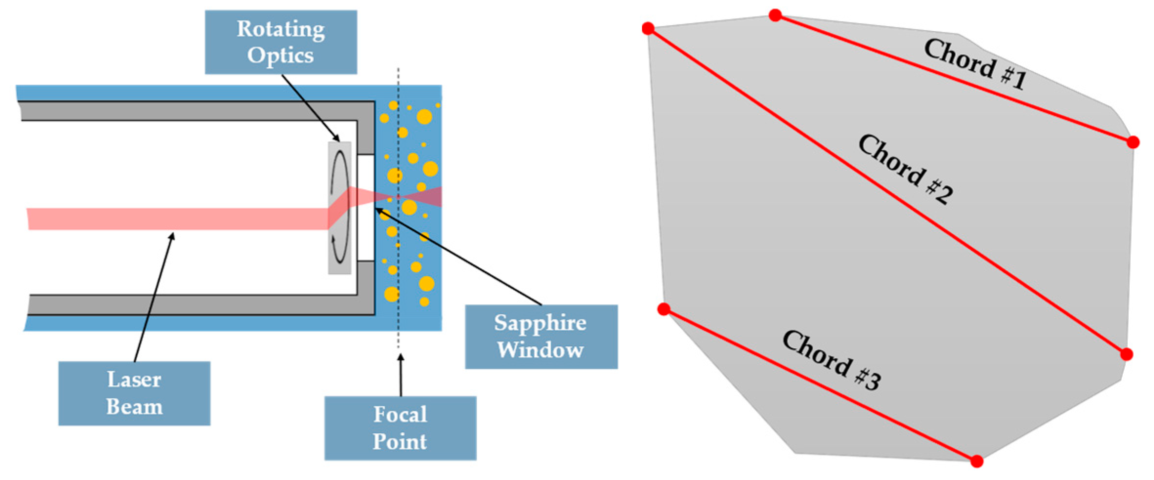

Figure 7.
Dynamic light scattering measurement working principle (adapted from [31]).
Figure 7.
Dynamic light scattering measurement working principle (adapted from [31]).
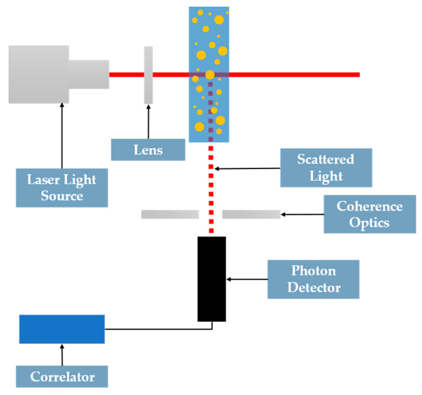
Figure 8.
Scanning electron microscopy (SEM) main component schematic (adapted from [39]).
Figure 8.
Scanning electron microscopy (SEM) main component schematic (adapted from [39]).
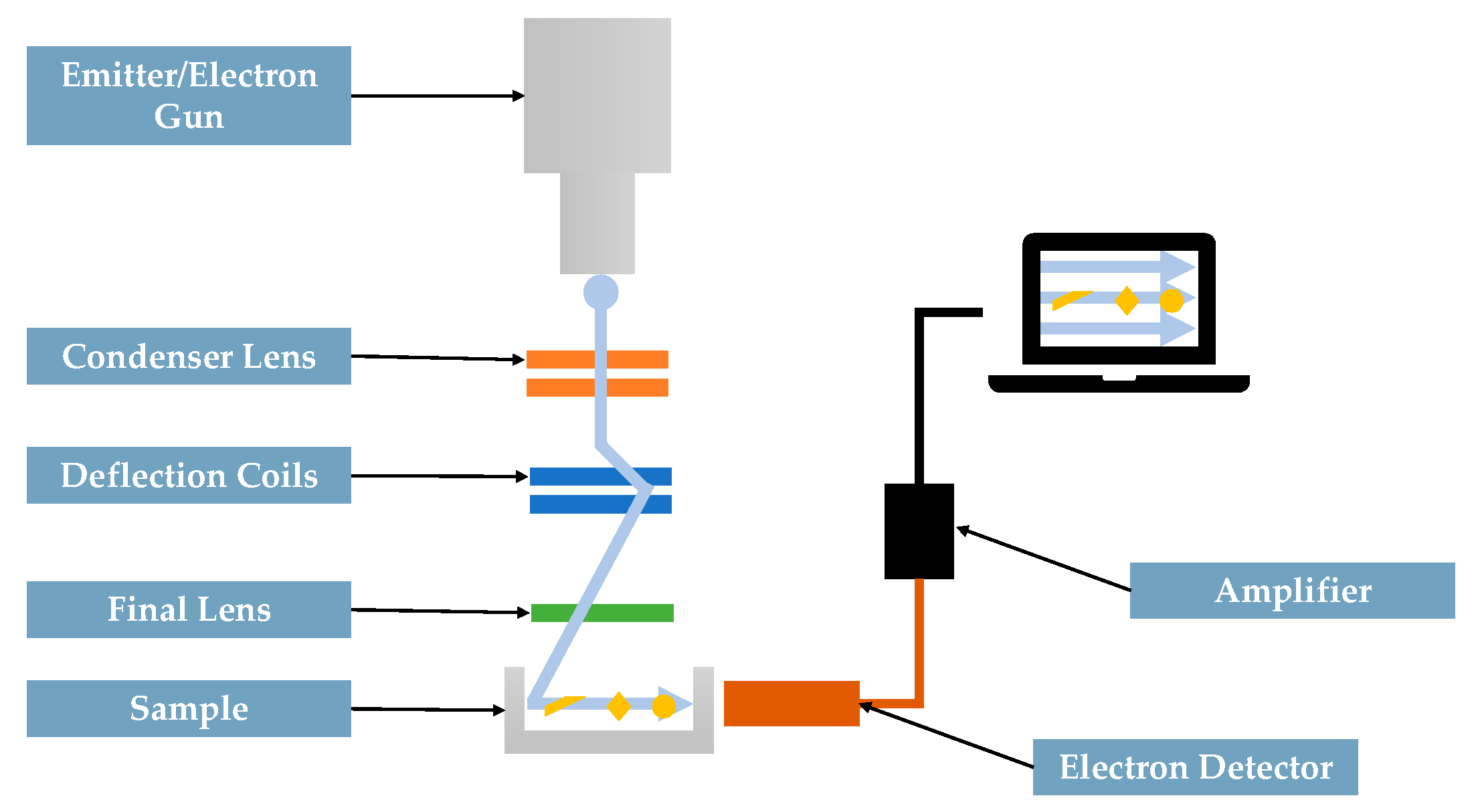
Figure 9.
Redmeter Rugged picture (taken from [42]).
Figure 9.
Redmeter Rugged picture (taken from [42]).
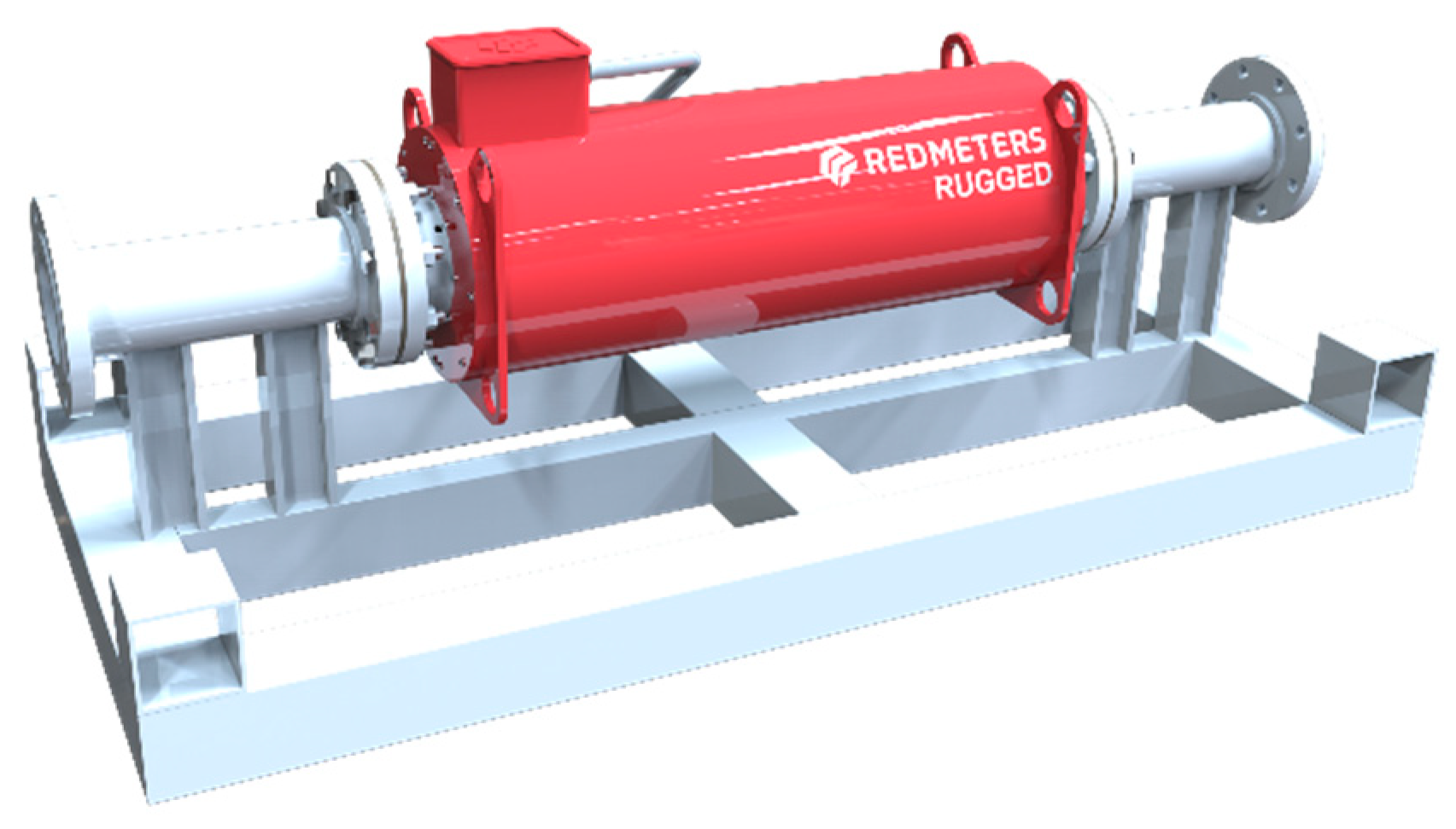
Figure 10.
Rhosonics SDM-1 model spool installation picture (taken from [43]).
Figure 10.
Rhosonics SDM-1 model spool installation picture (taken from [43]).

Figure 11.
Proline Promass F 300 Coriolis flowmeter model from Endress+Hauser for mass flowrate and density online measurements (taken from [44]).
Figure 11.
Proline Promass F 300 Coriolis flowmeter model from Endress+Hauser for mass flowrate and density online measurements (taken from [44]).

Figure 12.
Rotational (left) and tube (right) viscometer geometries (adapted from [47]).
Figure 12.
Rotational (left) and tube (right) viscometer geometries (adapted from [47]).
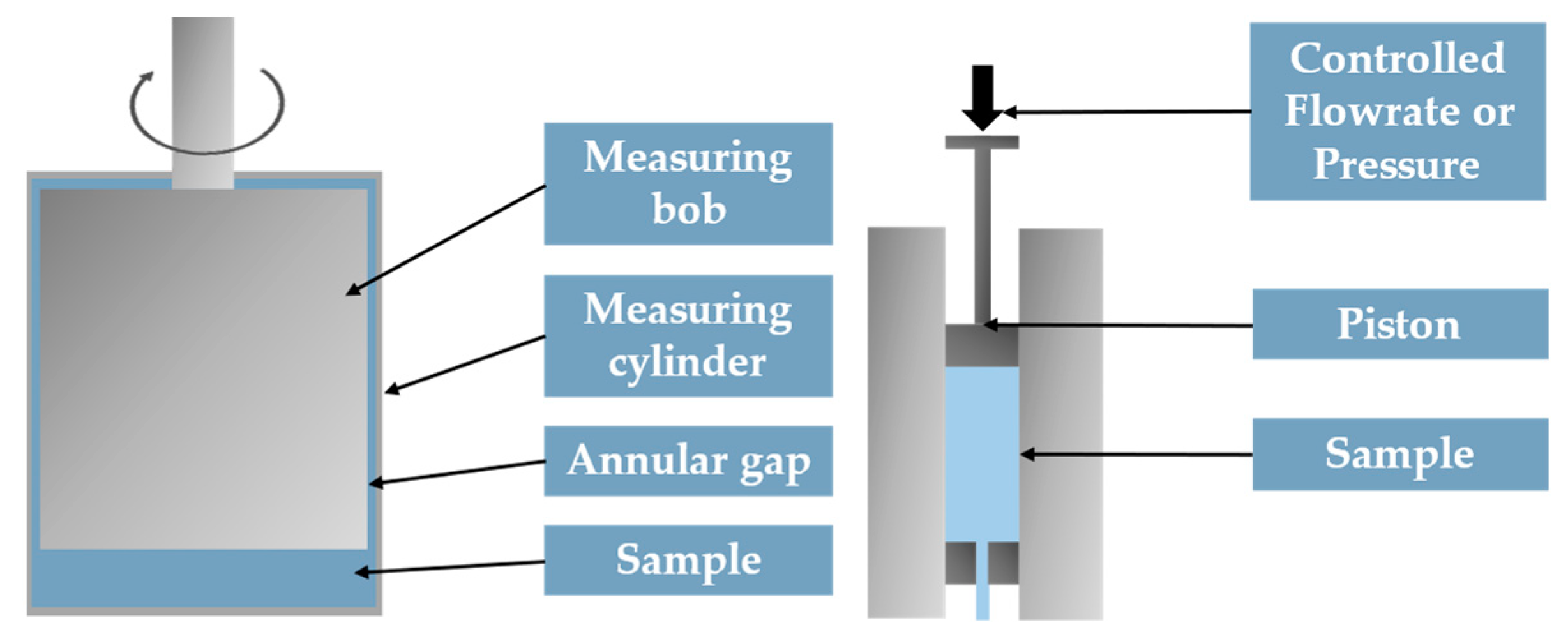
Figure 13.
Coriolis force working principle (left) applied for a rotating element flowmeter (right) (adapted from [51]).
Figure 13.
Coriolis force working principle (left) applied for a rotating element flowmeter (right) (adapted from [51]).
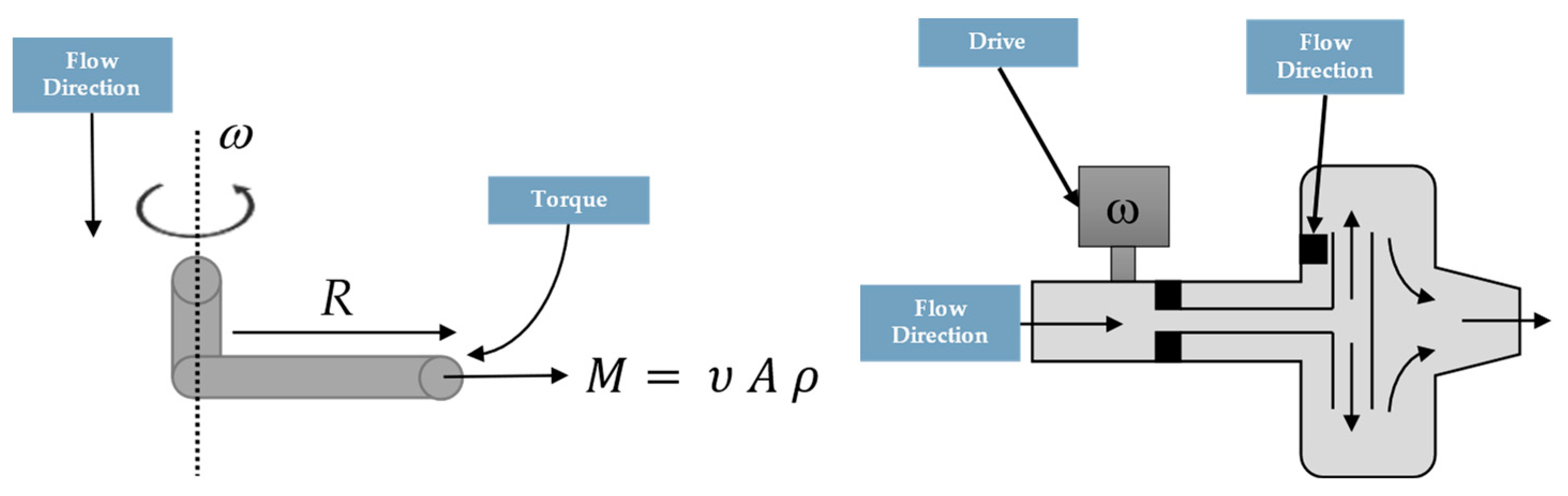
Figure 14.
U-shaped tube Coriolis mass flowmeter (CMF) (adapted from [5]).
Figure 14.
U-shaped tube Coriolis mass flowmeter (CMF) (adapted from [5]).
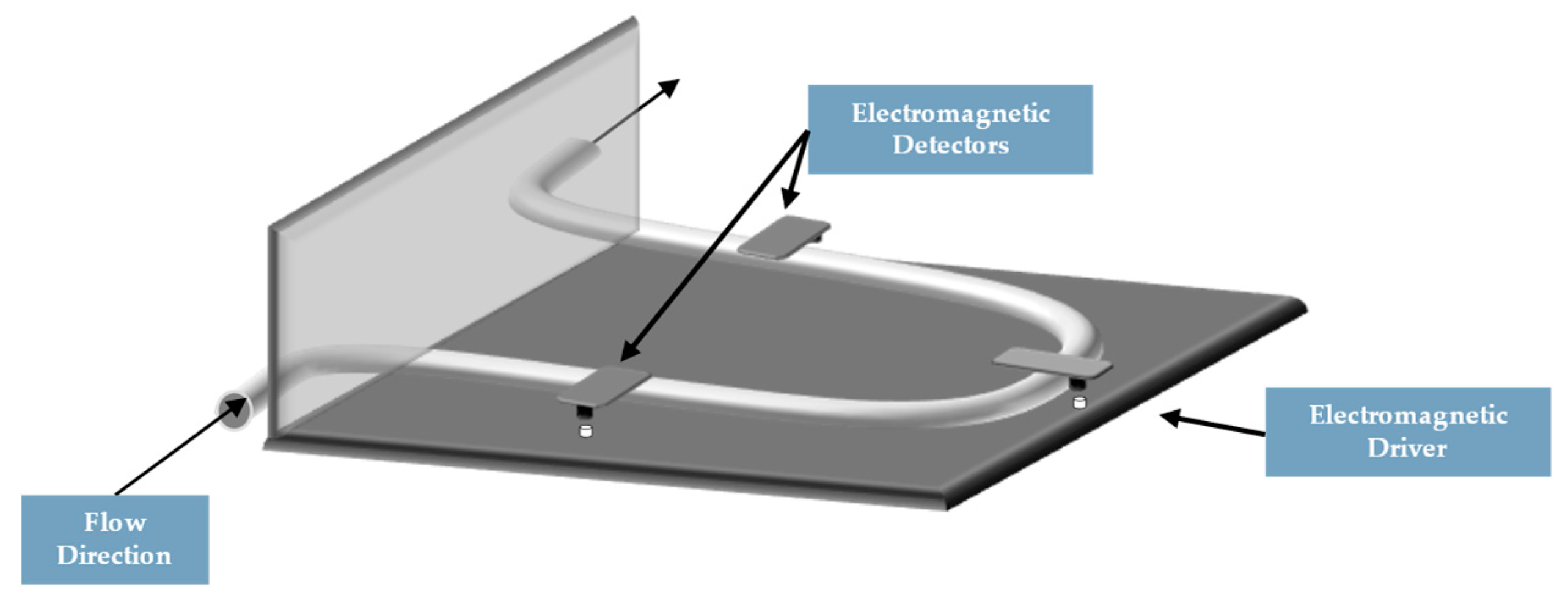
Figure 15.
Schematics of a magnetic flux flowmeter.
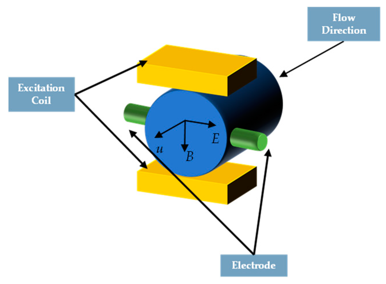
Figure 16.
Schematics of a venturi flowmeter.

Figure 17.
Conductivity probes with four-electrode (left) and six-electrode configurations (right) (adapted from [69,70], respectively).

Figure 18.
Electrical capacitance tomography system schematics (adapted from [76]).
Figure 18.
Electrical capacitance tomography system schematics (adapted from [76]).
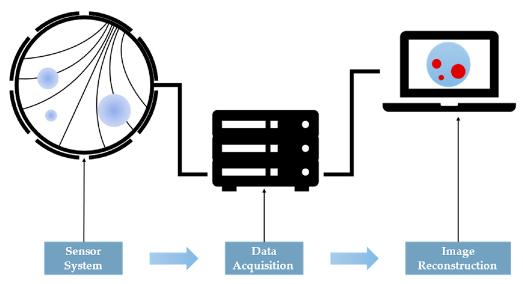
Figure 19.
Microwave tomography system schematics (adapted from [125]).
Figure 19.
Microwave tomography system schematics (adapted from [125]).
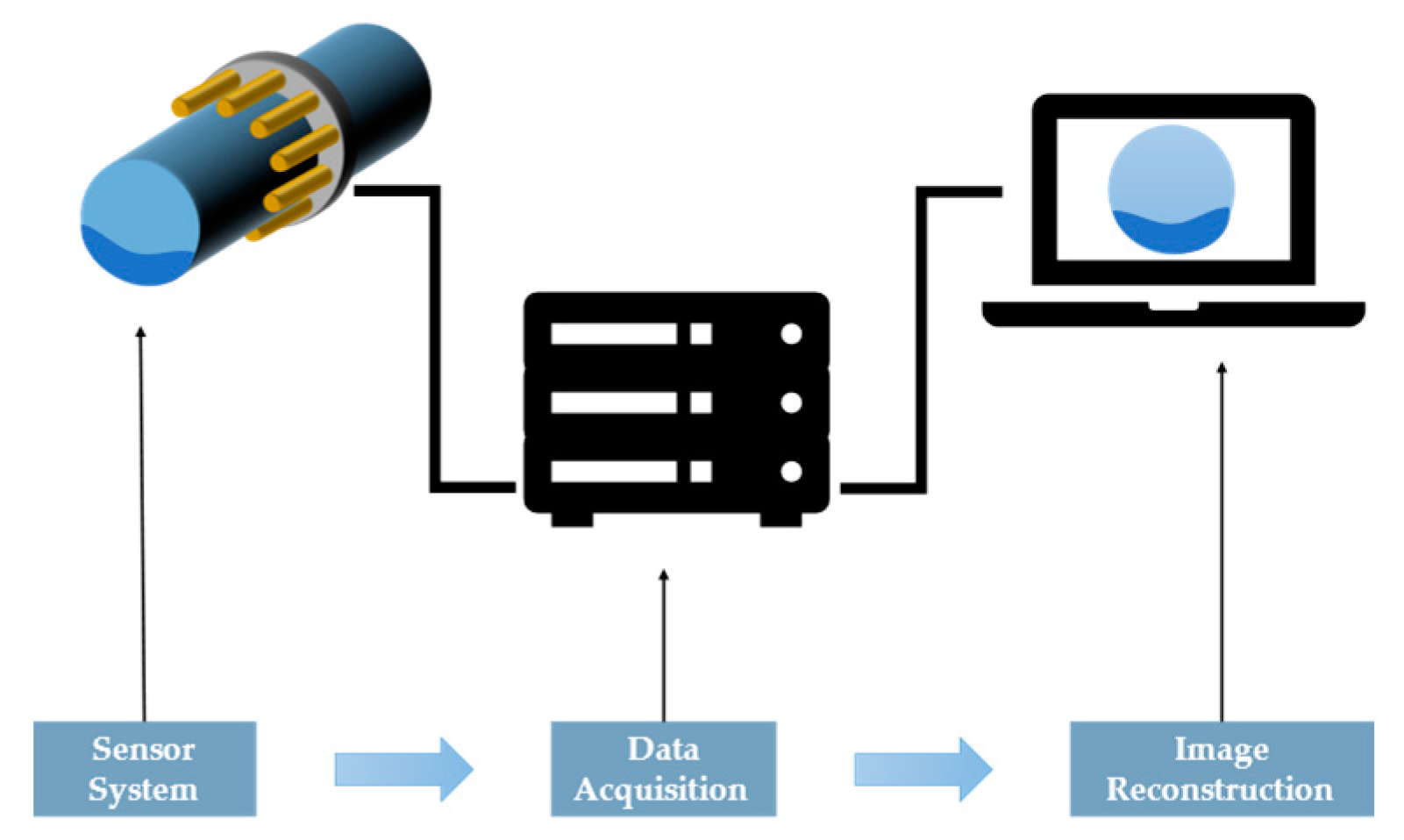
Figure 20.
Schematics of an active sensor system coupled with solid-liquid slurry flow.
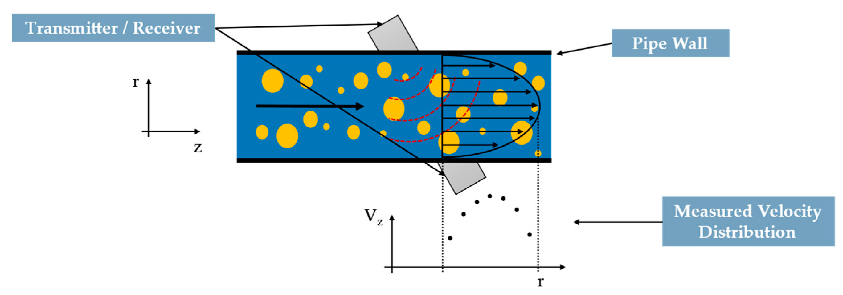
Figure 21.
Surface-Plasmon-Resonance Sensor (adapted from [140]).
Figure 21.
Surface-Plasmon-Resonance Sensor (adapted from [140]).

Figure 22.
Types of pitot tube: basic (left), static (middle) and averaging (right).

Figure 23.
Schematic of conductivity sensor structure (adapted from [146]).
Figure 23.
Schematic of conductivity sensor structure (adapted from [146]).

Figure 24.
Laser Doppler velocimetry system schematics.
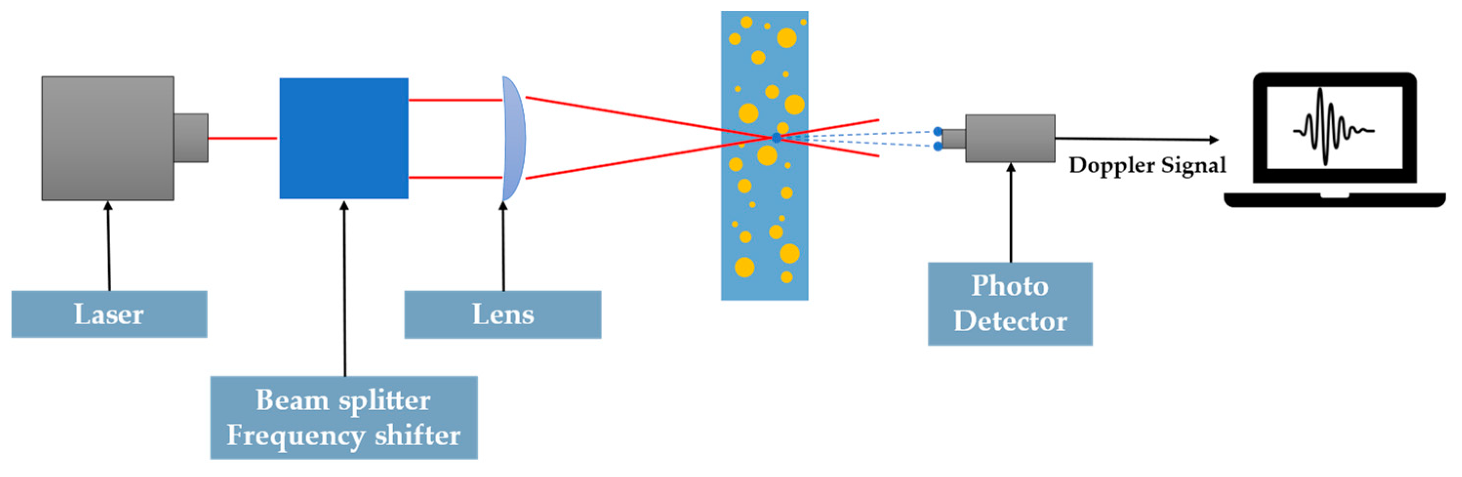
Figure 25.
Particle Image Velocimetry (PIV) system schematics.
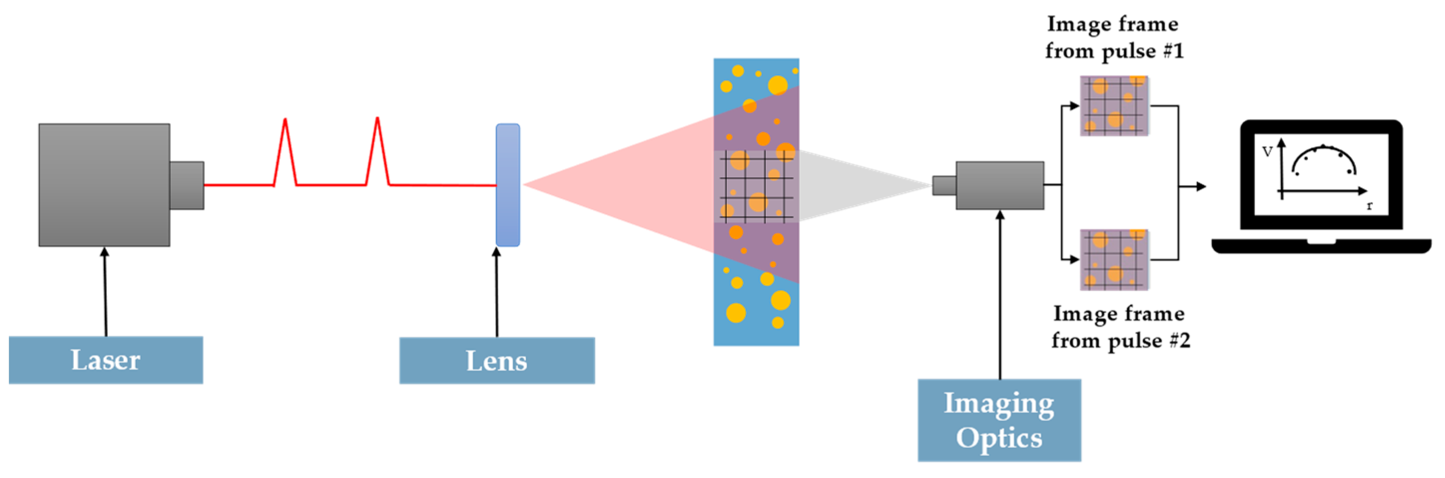
Figure 26.
Nuclear magnetic resonance tomography system schematics (left) and velocity profile measured in water-rayon fiber flow (right) (adapted from [134] and taken from [161], respectively).

Figure 27.
Gamma pilot M FMG60 model from Endress + Hauser for the radiometric measurement of level and density (taken from [173]).
Figure 27.
Gamma pilot M FMG60 model from Endress + Hauser for the radiometric measurement of level and density (taken from [173]).


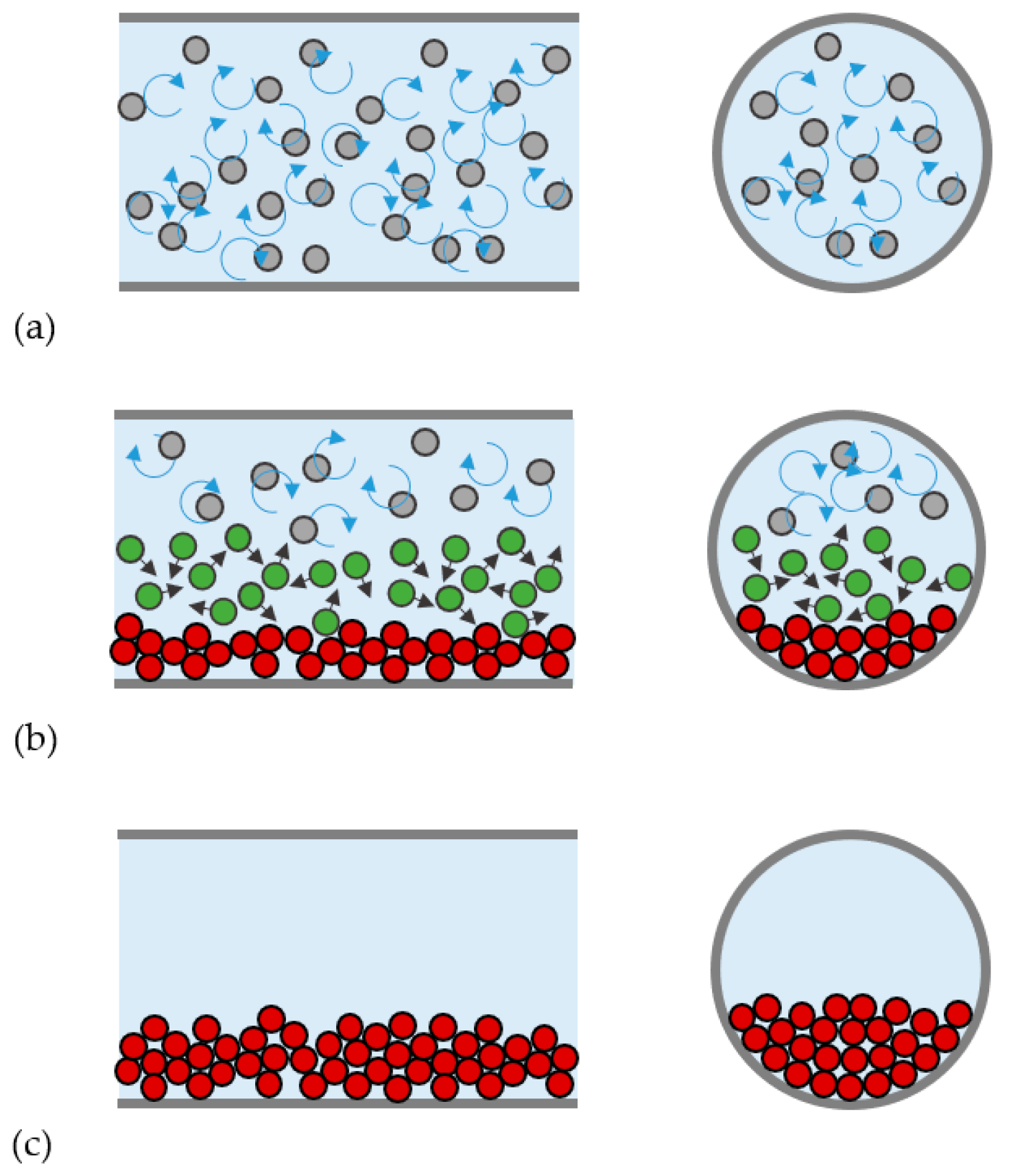
Table 1.
Comparison of electrical tomography techniques: ECT, EMT, and EIT (adapted from [100,101]).
| Tomographic Technique | Type of Sensor | Sensor Configuration | Electrical Properties Measured | Target Materials | Potential Industrial Application |
|---|---|---|---|---|---|
| Capacitance | Capacitive plates (non-intrusive and non-invasive) |  | Electrical permittivity (ε) and electrical conductivity (σ) | Electrically conductive liquid (water/saline, chemicals, minerals and pharmaceuticals) | Conveying monitoring, mineral transportation, chemical mixing, two-phase flow, bubble column, crystallization, and vortex monitoring |
| Electromagnetic | Coils (intrusive and non-invasive) |  | Electrical conductivity (σ) and magnetic permeability (μ) | Electrically conductive materials (water/saline, metals, minerals, magnetic materials) | Molten metal flow, two-phase flow, bubble columns and non-destructive testing |
| Impedance | Electrodes (intrusive and non-invasive) |  | Electrical conductivity (σ) | Dielectric materials (gas, oil, non-metallic powders, polymers) | Mineral transportation, fluidized bed, oil and gas flow and pharmaceutical #process monitoring |
Table 2.
Summary of advantages and disadvantages of characterization techniques for slurry flows process parameters.
Table 2.
Summary of advantages and disadvantages of characterization techniques for slurry flows process parameters.
| Measurement Method | Measured Parameter | Method of Operation | Advantages |
|---|---|---|---|
| Active Acoustics Ultrasonic Velocity Profiling | • Solid concentration • Velocity | • Alternating ultrasonic signals between transducers | • Non-intrusive • Sensitive to all objects in field • Rapid response time • Applicable to solid, liquid and gas flow • Directional sensitivity |
| Capacitance Sensor | • Solid concentration | • Solids cause variation of slurry permittivity | • Non-intrusive |
| Conductivity Probe Intrusive and Non-Intrusive | • Solid concentration • Fluid velocity • pH | • Potential applied across electrodes and a small current flow between electrodes depending on resistivity of slurry mixture | • Non-intrusive option • Sensitive to changes in conductivity |
| Coriolis Mass Flowmeter | • Mass flowrate • Volumetric flowrate | • Electromagnetic detectors sense vibration from electromagnetic drives on tube, measured based on Coriolis Force | • Unaffected by temperature, pressure, density and flow profile • Used with liquids, slurries, gases and two-phase liquid flows |
| Differential Pressure Drop | • Pressure drop • Velocity • Solids concentration • Flow patterns • Flowrates | • Effect of pressure fluctuations on velocity and concentration gradients | • Inexpensive • Well-known |
| Electrical Tomography | • Flow profiles • Solid and liquid velocities • Solids concentration | • Conductivity/permittivity measured between electrodes around pipe circumference | • Non-intrusive • Visualize flow • High speed imaging |
| Ionizing radiation-based techniques X-ray tomography Gamma-ray tomography Pulse Neutron Activation | • Velocity • Solid concentration • Rheological data | • Irradiation of sample using high-frequency electromagnetic waves, which propagate along straight lines | • Non-intrusive • High resolution images |
| Laser Doppler Velocimetry, Laser Doppler Anemometry Surface Plasmon Resonator | • Phase velocity • Turbulence • Particle loading | • Scattered laser light detected; amount of scattering based on solids in slurry • Surface plasmon resonance angle increases with an increase in solids loading | • Non-intrusive • Local velocity measurement of each phase |
| Magnetic Flux Flowmeter | • Volumetric flowrate • Slurry velocity | • Magnetic field generated perpendicular to flow, a potential difference generated by slurry flowing through the field | • Measure velocities of highly concentrated slurries |
| Microwave Sensor | • Solid concentration | • Interaction between microwaves and particles caused by relative permittivity | • Non-intrusive • Low sensitivity to electrical conductivity • Insensitive to temperature |
| Microwave Tomography | • Solid concentration • Mass flow measurements • Flow patterns imaging | • Dielectric properties of an object, such as dielectric constant or dielectric contrast, are measured through data from the scattered microwave field measured around the object | • Non-intrusive • Visualize flow• High speed imaging |
| Nuclear Magnetic Resonance Imaging | • Phase velocity • Solid concentration • Rheological data | • Distinguishing between atoms and molecules having different amounts of translational or rotational diffusion (Relaxation) • Distinguish between nuclei of atoms in chemically unequal sites (Spectroscopy) • Measures statistical averages of spatial and temporal scales | • Non-intrusive • Lack of directional preference • Micron scale resolution images • Immune to opaque media • Accurate measurements while acquiring a small number of points in several spatial dimensions in a short amount of time |
| Particle Tracking Velocimetry Particle Image Velocimetry | • Velocity • Turbulence | • Velocity measurements from the displacement of particles - PTV tracks the trajectories of individual particles while PIV tracks the mean displacement of a small group of particles. | • Non-intrusive • High speed imaging |
| Passive Acoustics | • Flow patterns • Velocity • Solid concentration • Presence of foreign objects | • Records sound generated by slurry flow through the pipe | • Non-intrusive • Penetrates opaque mixtures • Directional sensitivity • Rapid response time • Applicable to solid, liquid and gas flow |
| Pitot Tube | • Fluid velocity | • Pressure drop measurement between tube openings parallel and perpendicular to the flow | • Simple • Reliable • Inexpensive • Withstand high temperatures and a range of pressures |
| Scanning Electron Microscopy | • Particle shape • Particle size characterization | • Electron emission | • Quantification of particle shape and size descriptors from the 2D particles image (e.g., circularity, convexity, equivalent diameters, projected areas, perimeters, etc.) |
| Venturi Meter | • Volumetric concentration • Slurry velocity | • Constriction in pipe causes pressure drop due to increase in velocity | • Simple • Inexpensive • Ideal for homogeneous slurries |
Publisher’s Note: MDPI stays neutral with regard to jurisdictional claims in published maps and institutional affiliations. |
© 2022 by the author. Licensee MDPI, Basel, Switzerland. This article is an open access article distributed under the terms and conditions of the Creative Commons Attribution (CC BY) license (https://creativecommons.org/licenses/by/4.0/).
Share and Cite
MDPI and ACS Style
Silva, R.C. Experimental Characterization Techniques for Solid-Liquid Slurry Flows in Pipelines: A Review. Processes 2022, 10, 597. https://doi.org/10.3390/pr10030597
AMA Style
Silva RC. Experimental Characterization Techniques for Solid-Liquid Slurry Flows in Pipelines: A Review. Processes. 2022; 10(3):597. https://doi.org/10.3390/pr10030597
Chicago/Turabian StyleSilva, Rui C. 2022. "Experimental Characterization Techniques for Solid-Liquid Slurry Flows in Pipelines: A Review" Processes 10, no. 3: 597. https://doi.org/10.3390/pr10030597
Note that from the first issue of 2016, this journal uses article numbers instead of page numbers. See further details here.