Self-Adaptive Multi-Sensor Activity Recognition Systems Based on Gaussian Mixture Models


Intelligent Embedded Systems Lab, University of Kassel, 34125 Kassel, Germany
*
Author to whom correspondence should be addressed.
Informatics 2018, 5(3), 38; https://doi.org/10.3390/informatics5030038
Submission received: 8 June 2018
/
Revised: 13 September 2018
/
Accepted: 14 September 2018
/
Published: 19 September 2018
(This article belongs to the Special Issue Sensor-Based Activity Recognition and Interaction)
Abstract
:Personal wearables such as smartphones or smartwatches are increasingly utilized in everyday life. Frequently, activity recognition is performed on these devices to estimate the current user status and trigger automated actions according to the user’s needs. In this article, we focus on the creation of a self-adaptive activity recognition system based on inertial measurement units that includes new sensors during runtime. Starting with a classifier based on Gaussian Mixture Models, the density model is adapted to new sensor data fully autonomously by issuing the marginalization property of normal distributions. To create a classifier from that, label inference is done, either based on the initial classifier or based on the training data. For evaluation, we used more than 10 h of annotated activity data from the publicly available PAMAP2 benchmark dataset. Using the data, we showed the feasibility of our approach and performed 9720 experiments, to get resilient numbers. One approach performed reasonably well, leading to a system improvement on average, with an increase in the F-score of 0.0053, while the other one shows clear drawbacks due to a high loss of information during label inference. Furthermore, a comparison with state of the art techniques shows the necessity for further experiments in this area.
1. Introduction
The recognition of everyday activities is an active research topic, forming the basis for various fields of applications, such as healthcare [1], elderly care or context recognition (e.g., [2,3,4]). Their main goal is to translate low-level sensor signals into high level information about activities or even context, with context being the union of activities and surrounding environmental conditions. These techniques are broadly implemented in everyday devices, e.g., smartphones, smartwatches, earphones, jackets or shoes, and have been in use for quite some time. Thus, whenever, wherever a wearable is in your personal space, data from non-significant to sensitive are collected and evaluated by such devices. A limitation that still has to be overcome is the setup and configuration of interconnections, as they still happen manually. Depending on device and application, the user might implicitly be requested to be a configuration-expert.
Furthermore, current systems are prepared to work out of the box, with the broad field of Activity Recognition (AR) being narrowed down to explicit constraints, e.g., a fixed set of sensors, specific features and a predefined set of activities. Obviously, these limitations should be broken up, adapting to further input sources in a more contemporary manner by utilizing the flexibility and capabilities of current smart environments as, e.g., hinted in [5], where a outline on the further development of computing in our personal surroundings is given.
Currently, the integration of new sensors into working systems still forms a severe challenge. As such, it is worthwhile addressing and can be seen as a significant step towards self-improving processes with the goal to increase the overall robustness (following the definition of self-improvement given by Tomforde et al. [6]). To reach this goal, systems have to be able to incorporate previously unseen sensor sources into their running classification process. The research field connected to such claims is Opportunistic Activity Recognition (OAR) (cf., e.g., [7]), in which information sources are leveraged when they become available, i.e., where sensors just happen to be in place and deliver data.
The remainder of this article is organized as follows. An overview over current related work is given next, concluded by the identification of our research gap and the formulation of our contribution in the field of OAR. Section 2 describes the classification paradigm that was used in conjunction with our adaptation methods to new input sources. Afterwards, in Section 3, the experiments we conducted are described, along with the evaluation results. The outcome is then discussed in Section 4, before the article comes to closure with a short outlook.
1.1. Related Work
The adaptation of a system to incorporate additional input sources is a very specific application from the broader field of transfer learning. Utilizing the classification of transfer learning proposed by Pan et al. [8], our work is settled in the field of transductive transfer learning, with our domain being the aggregation of input sources (sensors). Even though our source and target domain are related (the former is part of the latter), the task of the system remains: classification of activities. The term domain adaptation, however, is used controversially by different groups. The works of Jiang or Daume III [9,10] introduces a term of domain adaptation that also fits our approach. The authors described domain adaptation from one domain to another, which in our machine learning context boils down to the adaptation from one feature space to another. This terminology was first established in the field of text classification, but can be transferred to the domain of Activity Recognition (AR) in a straightforward way.
A different approach following the same domain adaptation goal was proposed by Duan et al. [11]. Their method starts with the projection of the source and target feature space into a common subspace, in which a standard learning algorithm is applied. Tested on a computer vision dataset with up to 800 features, the authors showed the feasibility of their approach. Nonetheless, two major differences to our work have to be pointed out: (1) While the authors only have an explicit subspace between domains, we assume that subspace to be exactly the original input space. (2) The dimensionality of computer vision data is often very high, even if compared to AR data with multiple features from several sensors, as we investigated.
The research field of Activity Recognition itself is too wide to be covered entirely here and, as mentioned above, overviews can be found (e.g., [2,3,4]). Furthermore, Chen et al. contributed a study that classifies different approaches, depending on sensing devices and whether they are model-based or data-based [12]. Data-driven approaches are distinguished depending on the sensing “device”: either sensor-equipped objects or sensors attached to persons deliver the data. Depending on the approach, either the human–object interaction is used as input, or the recognition process is fed by human motions. Either way, activity predictions are the output of the system. Model-driven approaches are characterized as relying on either discriminative or generative modeling techniques. Both terms are apprehended below. Besides the categorization of techniques, no comparative evaluations have been done whatsoever.
In contrast to that, Lara et al. [13] included an overview of evaluation results in their study. In terms of categorization, they differentiated four kinds of attributes: (i) environmental attributes; (ii) acceleration; (iii) location; and (iv) physiological signals. Regarding further properties of recognition systems, they also argued about energy consumption of devices, obtrusiveness, common features, classifiers and evaluation measures. The study is concluded with the analysis of different online-AR-systems. However, despite the large amount of investigated papers, all approaches rely on static input spaces, neither sensor failure nor the adaptation to new input sources is discussed.
Further narrowing down our research, AR based only on wearable sensors has to be mentioned. As the number of available sensing devices increases, especially smart watches and alike pervading our daily lives, several groups perform research in this field (e.g., [14,15]). Even though this field comes close to applications we have in mind, they follow a static setup, with neither adaptations nor improvements during runtime. The authors of [16] separated kinds of sensing from a privacy point of view. Participatory sensing is defined as a sensing task, based on information of people willingly sharing sensed information from their personal surroundings, which in the end benefits their own sensing task, as other participants are encouraged to share information, too. In the author’s sense, opportunistic sensing can be separated from participatory sensing, as the offered data may not benefit themselves, but other people. In both cases, users have to explicitly approve the usage of their data.
The field of wearable sensors is also the enabler for the class of AR we find our work in: the field of Opportunistic Activity Recognition. First described by Campbell et al. in [17], it focuses on opportunistic sensing, a kind of sensing that exploits all sources that become available to a system. The group envisioned the usage of multiple sources that become available under certain conditions, i.e., sensing applications specific to a given task, sensors within a certain area or sensors that are available in a specific time window. The (changing) availability implies a non-static input space, offering sufficient sensor coverage along the movement path of experimentees (custodians).
Bannach et al. studied techniques to integrate previously unseen sensors into a running classification system autonomously [18,19]. Investigations are limited to a decision tree classifier, with the advantage that new sensors lead to the replacements of leaves in the tree by new subtrees for the extended dimensions. Experiments are successfully conducted on artificial datasets as well as real sensor datasets, showing that an adaptation from one input dimension to two input dimensions can be done and will on average do more good than harm. Throughout their work, four extensions to the method are built on top of each other and used to improve the achieved results significantly. However, it can be seen that the method heavily relies on dataset specific heuristic findings, which was also stated by the authors.
Shifting the focus from scenarios towards specific solutions, several groups are worth mentioning. The usage of discriminative models is prevalent (cf., e.g., [20]), compared to the usage of generative modeling techniques [21]. Discriminative models are inferred from training data, model the decision boundaries directly and usually need only little computational effort for processing. The major downside, however, is their black box behavior, which is hard to interpret for humans. Furthermore, no information on the data modeling is available, i.e., parameter changes can greatly influence the prediction result, but the parameter influence may seem erratic and inexplicable, even to experts. Opposing to that, generative models capture the structure of data and thus are a more natural way of describing (the structure of) data. Under certain assumptions, they are also well-interpretable by human experts (cf. [22]). It is safe to say that, the greater is the number of training samples, the better is the structure-coverage by the model. With some extension, a generative model can be used as a classifier, e.g., by assigning class labels to model components.
A combination of both approaches was proposed by Jordan [23] and later refined by Raina et al. in [24]. Working with a logistic regression as discriminative part and a Naive Bayes classifier as generative, a classification problem is addressed. Their data were text-based and they performed a comparison of generative and discriminative techniques, stating that the generative models performed better than their discriminative counterparts. Such an outcome is never supported by other researchers, but instead often reversed, e.g., by Huỳnh and Schiele or Chen et al. [12,25]. The group around Schiele also combined a generative model to capture structure in data and a Support Vector Machine (SVM) as realization of a discriminative model, to solve an AR problem. However, their combination works on a static input space, which makes the approach incomparable to our adaptive approach.
The authors of [26] connected a combination of Hidden Markov Models (HMMs) as generative part to Conditional Random Forests (CRFs) as discriminative part to recognize activities. Their method models the temporal relationship of observations by means of an HMM and a CRF in parallel. The used datasets are several days long; however, the input space does not change during experiments. Furthermore, this technique and the ones discussed above are rather more ensemble-based than true hybrid solutions towards recognizing activities.
The authors of [27] stated that they developed a collaborative, opportunistic activity recognition framework, to include or replace elements from six available on-body sensors. After (pre-)classifying micro-activities, they argued that a more suitable classifier for the macro activity can be chosen. Interestingly, their approach should work with any type of classifier, not only the proposed maximum entropy classifier that was first introduced by Berger et al. [28]. However, it turns out that the adaptation takes place via fixed rules from a configuration database. That database is kept rather mysterious, as it is not described at all, but obviously the most interesting part of the work (with respect to autonomous adaptations). In addition, the parameterizations of comparison-classifiers are described insufficiently, thus no quantitative conclusions about the quality of their proposed classifier can be drawn. They also analyzed the energy consumption of systems issuing all sensors and systems issuing a selected set of sensors. This point is quite important, as batteries of embedded devices only have a limited amount of energy available.
The work of Villalonga et al. provides a much more detailed description of adaptation techniques [29]. The authors introduced an ontology-based system to include and replace sensors via selection techniques. Based on a predefined ontology with different properties, a set of candidates is made available. From that set, based on heuristics, one candidate is chosen and integrated into the system. However, it is a very restrictive policy, as only certain sensors can replace others: if no relation between two sensors is available in the ontology, a replacement is not considered. One assumption they made seems rather valuable, i.e., the assumption that each sensor offers a self-description, so that systems know about the availability of that sensor and how to exploit its data. However, the assumption that a sensor “knows” its on-body location seems a bit off, as that alone requires either very precise recognition techniques within such a unit, or a mandatory bound between sensor and sensor location.
Introducing an intermediate level of abstraction, Rokni and Ghasemzadeh worked on the extension of AR systems [30]. Their approach introduces sensor views, i.e., the aggregation of one or even several sensors in a group (view). They assumed that sensors can only detect events that happen close to them, even though that assumption does not always hold up (e.g., inertial measurement units (IMUs) mounted to the upper arm or chest can very well recognize footsteps). Given prior class probabilities that are estimated from the training data, the adaptation process covers the refinement of a classifier during runtime, with the major challenge of label inference being solved as follows. Observations in the extended sensor view are first clustered via k-means and then each cluster is assigned a label. The number of activities is assumed to be k, however that assumption hardly holds up on real data. The assignment is seen as a matching problem in a bipartite graph, with one group of nodes being the classes, another group of nodes being the clusters and the edges being weighted connections between them. The matching is done via the improved Hungarian algorithm [31]. The knowledge base for distributing labels is taken from the original classifier (more specific: the prior probabilities of each predicted class are used) and evaluations were done as transfer learning applications with one starting sensor and one target sensor. The labels used for inference are called semi-labels, but are just multinomial distributions with gradual class affiliations (e.g., in a three class problem, such a semi label could be ). After label inference the classifier adaptation happens as a fully supervised classifier training. The transfer from systems with one sensor to systems with another sensor is one restriction, even though a broader vision of sensor views was mentioned. Furthermore, the quality of the retrained system highly depends on the quality of the original classifier, which does the heavy lifting in the label inference process.
Wang et al. formulated an approach based on extreme learning machines [32]. They focused on a set of four IMUs that were distributed on a subject’s body’s right ankle, waist, wrist and right on top of the bellybutton. They investigated the ability of adapting a trained system to an unknown sensor location. To simplify the problem, the investigated accelerometer signals were transformed and just the magnitudes of the signals were used. This greatly reduces the dimensionality and makes the signals independent from the actual sensor orientation. On the eleven features that are extracted, Principal Component Analysis (PCA) is performed, however, it is unclear how many resulting principal components are processed further. A kernel is then created, based on a self-defined comparison measure for PCA-transformed feature vectors and a label inference confidence is computed, based on the ground truth labels from data. Those labels are available for the training data, however, in an actual application, not for the adaptation data (the confidence is still computed in the same way). The samples with highest confidence are used for retraining the classifier on the adaptation data. As interesting as the overall approach is, even formulating the adaptation process in a linear form, it is not yet feasible, i.e., relying on ground truth labels, which are not available for adaptation data. Furthermore, adaptations are just investigated from one sensor to another sensor, with no extension of the input space but rather a transfer between input spaces.
Münzner et al. recently investigated an approach that uses Convolutional Neural Networks (CNNs) to recognize activities and perform adaptations [33]. Due to the paradigm, no features are extracted, as network weights are used to model the influence of signals. The group investigates different sensor fusion techniques (the fusion at different convolutional layers) and their influence on recognition performance on two datasets, one newly recorded (Robert Bosch Krankenhaus, RBK) and the PAMAP2 dataset (which was used in this work, too). Investigations show how well different sensor fusion techniques perform, but not how an adaptation during runtime can be done. Furthermore, the results have to be looked at very carefully, as, firstly, no cross-validation (or alike) is done, while training and test set are the same. Secondly, some properties of the datasets are changed, e.g., an interpolation from 1 Hz signals to 100 Hz signals is performed for synchronization purposes and the class priors are changed by repeating samples from underrepresented classes.
The work of Morales et al. [34] is also from the field of deep learning, but released one year earlier. They trained a deep CNN and transferred parts of it to adapt to new target domains, with the goal of enabling adaptations between users, application domains or sensor locations. After training an initial CNN on a training dataset, a certain percentage of held back adaptation data is used to train a new network. That new network, however, re-uses different numbers of convolutional layers from the initial CNN, freezes them and retrains the remaining layers with that said percentage of data. Thus, a part of processing by the network is constant (e.g., the feature representation of the foremost layers), while the target domain specific layers (rearmost layers) are adapted. Evaluations show that, with five convolutional layers in a network, the greater part (three or four foremost) should be kept constant, and the remaining should be (re-)trained to perform an adaptation from one user to another on the same target domain. Transfers between domains, i.e., different datasets, were investigated, but have to be considered less successful. The overall idea is very promising, with a lot of parameter finding still possible for further optimizations. The adaptation between domains or to new features, by freezing certain layers of a CNN, are proven to work.
Rey et al. introduced a novel mechanism to autonomously integrate a new sensor into an AR system [35]. They started with a readily trained classifier as we do. After collecting a certain number of observations from the extended input space, the adaptation happens in several steps, starting with the creation of a similarity graph on the new observations. Afterwards, the labels for those new observations are predicted by the initial classifier, after projecting the observations back into the original input space. Those labels are then propagated to all new observations based on the similarity graph. With fully labeled observations in the extended input space, a new classifier is trained fully autonomously. The approach is very promising and proven to work on real life datasets, especially with more than one dimension added. It is also not confined to a specific type of classifier.
1.2. Research Gap
One major drawback that can be seen in most related work is the fixed nature of the input space (cf., e.g., [14,15]), neither sensors are failing nor new input sources become available in discussed papers, only Bannach [19] and Rey and Lukowicz [35] truly tackled that problem. It can also be concluded that most approaches have an idea on the expansion of a system to cover further input sources, however, they either rely on ground truth labels (something that is not available in real life scenarios; cf. [32]) make assumptions that do not hold up on real life datasets or describe systems with narrowly defined rules for integrating/replacing sensors in a very restrictive manner [30]. Another gap we want to overcome is the missing link between observed structure in data (captured via generative models) and the addressed classification task (discriminative models). Both should work in conjunction, not side by side or in competition.
This article addresses the problem of a variable number of input sources and how to handle an input space that is extended with additional input sources. We contribute a realization of the concepts described in [36,37,38]. Data are captured and modeled in a generative manner, with all its enriching information at hand (uncertainty estimations, probabilistic class predictions, etc.). The key contribution of our work is the provision of methods to autonomously extend Multi-Sensor systems based on probabilistic, generative models with new sensors during runtime, which is proven to work on a well established AR-dataset.
2. Methods
We investigated the adaptation of generative, probabilistic classifiers, namely Classifiers based on Mixture Models (CMMs), as from a machine learning point of view, AR is a classification task. An overview of this kind of models is given in the following section, while more detailed explanations can be found elsewhere (e.g., [39,40]).
2.1. Classifier based on Mixture Model
The classifier is based on a Gaussian Mixture Model (GMM) that estimates the density of a given training dataset. The estimation is done with several, multi-variate normal distributions (components) that have class labels associated with them and are summarized in a linear combination. Thus, given an input sample, a class prediction can be made. The choice of Gaussian components as a basis is motivated by the generalized central limit theorem, which states that an infinite sum of independent samples drawn from an arbitrary distribution (with finite mean and variance) converges to a normal distribution [41]. As sensor signals always come with noise, the assumption of such signals to be normally distributed is quite obvious.
In a scenario with C different classes, the desired output can be formulated in a Bayesian manner as ; the probability for a class given an observation . With J overall components in the model and each component having a class label (conclusion), the posterior distribution to predict a class, given an input sample , can be formulated as:
With that notation, is the probability for class c, the class prior, that has a multinomial distribution and is derived from the training data. The term represents the probability for a sample , given component j (and with the component, its associated conclusion c). The expression also has a multinomial distribution, with each parameter being the mixing coefficient for component j, which represents the weight component j has on class predictions of the model. Note that all mixture coefficients must be positive
and they must sum up to 1:
Finally, the term is the probability of sample given the current model. This is also known as the generative property of these models; meaning that data points drawn from these models’ distributions are indistinguishable from the data that were used to train the model.
Each component itself is a multi-variate normal distribution , characterized by mean and covariance matrix. In an input space with d dimensions, the mean can be written as and the covariance matrix as
The entries in a covariance matrix influence the overall form of the Gaussian bell curve of component j, so that even complex dataset-forms can be covered. Furthermore, the matrix can be inverted, is symmetric and positive-semi-definite. Normal distributions also have a marginalization property (cf. [39]), which we exploited for our adaptation. Given a normal distribution, the partition into disjoint subsets (dimensions) gives normal distributions. Marginalizing dimension in the above example would result in a distribution with mean and covariance matrix
Please note that this property can also be utilized the other way around: Given a -dimensional normal distribution, the addition of a univariate normal distribution (with appropriate adjustments of the covariance matrix), ultimately results in a d-dimensional normal distribution. Taking these thoughts one step further, it should be clear that they also apply to a GMM, as a GMM is just a linear combination of normal distributions.
Shortly summarized, each component in a GMM has a specific form defined by its mean and covariance matrix, while its weight on overall predictions is given by an associated mixture coefficient. Class labels are associated to each component, and a weighted sum of all component labels depicts the system output for a given observation. The density function of a GMM with J components can finally be written as follows:
A Classifier based on Mixture Model can be trained via Variational Bayesian Inference (VI), a training algorithm first proposed by Bishop [39] and successfully applied to GMMs in, e.g., [42]. Given a labeled training dataset, the algorithm follows a Bayesian approach to iteratively fit a GMM to the data. It can be seen as a generalization of Expectation Maximization (EM), however, with the major advantage that it can prune components during training, which (1) reduces model complexity; and (2) does not need a specific number of components a priori. Furthermore, the major drawback of EM can be avoided, as no more singular covariance matrices for components occur during training.
Given a d-dimensional input space , a training dataset and a readily trained CMMbase, the question how it can be adapted to new input sources is clarified next. Given enough samples, the next step depends on the adaptation method. In principal, two different approaches can be taken, one based on the initial classifier (model-based) and the second based on the initial training data (data-based). The adaptation process starts with new observations in a -dimensional input space , honoring the condition .
2.2. Data-Based Adaptation
In short, this approach trains a density model, infers labels in the original input space and then switches to the resulting classifier.
The first step is the creation of a new density model in the extended input space . The training of such a model, say GMMadapt, is done unsupervised, again via VI. Given that density model, the marginalization property is issued as follows: The model is backprojected to the original input space , by marginalizing all k dimensions that extended the original input space, resulting in . Labels for this density model are then inferred, using the training dataset : Each sample of is associated to the component with the greatest density. From the set of all associated samples, the label that is most widely spread among the samples is taken as label for the component (winner-takes-all approach). After inference, the labeled model is forwardprojected to the extended input space , resulting in CMMadapt. That classifier is then used and issues all input dimensions available to the system. Figure 1 illustrates the described process with a simple example, adapting a system from one input dimension to two.
2.3. Model-Based Adaptation
This approach trains a classifier in a fully supervised manner, and afterwards labels for observations in the dimensional input space are inferred.
All collected observations from are backprojected to the original input space by omitting the k new dimensions. The original classifier CMMbase is then used to predict labels for these data points in . Afterwards, the labeled data points are forwardprojected to the extended input space. In the next step, a new classifier CMMadapt can be trained fully supervised in the extended input space, again via VI. That new classifier then replaces CMMbase and from then on works on all input dimensions available to the system.
3. Results
The dataset we used to conduct our experiments is the PAMAP2 dataset, introduced by Reiss et al. in 2012 [43,44]. It comprises data from nine subjects, eight male and one female, aged 27.2 ± 3.3 years. All of them performed a protocol of the following 12 activities, resulting in approximately 10.7 h of collected data: lie, sit, stand, walk, run, cycle, nordic walking, ironing, vacuum cleaning, rope jumping, ascending stairs and descending stairs. However, one subject was found to miss some activities. To avoid diluting the evaluation results (as misclassifications of these missing activities would never occur), Subject 9 was taken out of the dataset.
Four sensors were used to collect data, three IMUs and one heart rate monitor. From each IMU, the accelerometer and gyro data were used, each with three degrees of freedom. The raw data were re-sampled to 32 Hz, as this frequency was found to be enough for detecting everyday activities (cf. [45]). Feature extraction took place on sliding windows that contained 128 sensor-values (which correspond to 4 s of data) and were shifted for 1 s (32 values), before the next feature-computation. Then, one measurement for each second was stored. From each sliding window, mean and variance of each sensor axis were computed as follows, forming 12 features for one IMU:
- mean
- variance
with N being the number of samples in the sliding window and being the vector of raw sensor signals at position n. After feature-extraction, a standardization was performed, so that each feature was adjusted to a mean of 0.0 and a standard deviation of 1.0.
From a system’s perspective, the addition of a sensor involves the addition of each feature extracted from that sensor’s signals, thus extending the system by one IMU can mean an extension of the input space by as many as 12 input dimensions (three acceleration signals, three gyroscope signals, and two features for each dimension).
The sensor adaptation experiments involved (1) the selection of a set of sensors to start with (the baseline); (2) extending the system by one sensor; and (3) comparing the adapted system to the baseline. The base system was extended and evaluated with each of the remaining sensors separately and evaluation results were then averaged, to get resilient results. We chose to use the F-score for evaluations, as it expresses in detail how precise and sensitive a classifier works. Originally, the F-score applies to binary classifiers only, where it is defined as the harmonic mean between precision and recall:
Precision is the ratio of true positives to predicted positives or, in terms of true/false positives/negatives:
It describes how precise a classifier predicts a class, e.g., which portion of predicted class members actually belongs to that class. Recall is also known as sensitivity and describes the ratio of the number of true positives to the overall number of class members in the dataset. In terms of true/false positives/negatives, it is defined as follows:
It describes how sensitive a classifier correctly predicts labels for a class, which fraction of all class members was predicted correctly. To apply this score to multi-class scenarios, two ways are possible: One is averaging the F-scores of all one-vs.-one classifiers in the problem (in the case of C classes values have to be averaged). This approach leads to the micro-average F-score, which is equal to the common accuracy metric. However, as an alternative the macro-average F-score is computed as the harmonic mean of averaged precision and averaged recall. The macro-average F-score is used as a metric for our experiments, because the accuracy has the large drawback that it implicitly assumes the same number of samples for each of the C classes in the training data. This assumption is violated in most real life datasets, so that the message from evaluations with this metric becomes very vague. For example, given 1000 samples and three classes Null (800 samples), Event 1 (100 samples) and Event 2 (100 samples), a “classifier” that always predicts Null (no matter the given sample), will have an accuracy of 0.8 right away, while its macro-averaged F-score will just be
Obviously, for metrics between 0.0 (bad performance) and 1.0 (great performance), a value of 0.8 is more misleading than a value of 0.267, for a “classifier” that just outputs class Null. Sokolova et al. discussed further details on the F-score and its advantages compared to the accuracy [46].
Experiments were conducted in three-fold cross-validation, as a more fine-grained division would lead to overfitting classifiers. For parameter optimization, a random-search with five different parameters was issued. Parameter optimizations that were used relied on a comparison of the logarithmic likelihood of the model on the training data as criterion.
3.1. Benchmark
To measure the feasibility of our overall approach, we investigated the quality of the algorithms proposed by Reiss and Stricker [43], using all sensors from the start. Please note that: (1) We used different features than the authors described above; (2) We used a different, more meaningful measure for the comparison. Figure 2 shows the comparison on test and training data between the author’s tested methods and our approach. It can clearly be seen that our approach is competitive, i.e., the F-scores are in the same range as the other methods. However, our proposed CMM is a more powerful approach (as it is a generative model) that captures data structure besides the classification properties and that comes with the ability of integrating additional dimensions.
3.2. Baseline
The baseline case involved an evaluation with the starting set of sensors only. From four available sensors, just one, two and three were chosen. When selecting one out of four sensors, there are four possibilities to choose, selecting two out of four reveals six possible combinations and so on. Selecting four sensors out of four results in just one combination, however, that case can not be adapted, i.e., no further sensor can be added. That case can be found in Section 3.4. The results for this baseline case are computed on sets of four, six and four sensor combinations, respectively (14 sets overall). Each time the data were cross-validated, parameters were optimized and the experiments were conducted for each subject, thus 1680 evaluations were done. The results serve as a lower bound in system performance; every adapted system is expected to perform better than this.
3.3. Extension
For our experiments, we evaluated each baseline system with one of the remaining sensors added, i.e., starting with just one sensor, three evaluations of adapted systems took place: baseline plus remaining sensor 1; baseline plus remaining sensor 2; and baseline plus remaining sensor 3. Four baseline sensor sets with just one sensor can be formed, each time with three other sensors being available. That sums up to 12 experiment sets, which were handled by two different adaptation strategies (cf. Section 2.2 and Section 2.3), resulting in 24 experiments. As a three-fold cross-validation was done, five parameter-sets for the density estimation were investigated and data from eight subjects was used, the overall number of experiments for a baseline sensor set of just one sensor increased to 2880. Regarding two baseline-sensors, six different sensor sets can be chosen to start, with two sensors being available for adaptation. Again, this results in 12 experiment sets, and, with regard to adaptation strategies, folds, parameters and subjects, ultimately results in 2880 experiments for a baseline sensor set of just two sensors. Going through all combinations, three sensors in a baseline set can be formed in four variants, but have only one additional sensor available, which leads to 960 experiments. Overall, 6720 evaluations were done to get reliable numbers on the extensions.
3.4. Comparison
Comparison experiments were done on the adapted sensor systems as follows. From the start of the experiment on, all data from all sensors (baseline set plus additional sensor) were available. Thus, the sets had data from two, three or four sensors available from the start. With sets of six, four and one element being created from four available sensors (11 sets overall), considering the cross-validation, parameter optimizations and the number of subjects, 1320 experiments were evaluated. The results can be seen as an upper bound for the expected improvement of adapted systems. Please note that the baseline for two sensors forms the comparison case for systems with just one sensor, the baseline for three sensors is the comparison for two sensors and so on.
3.5. Evaluation Results
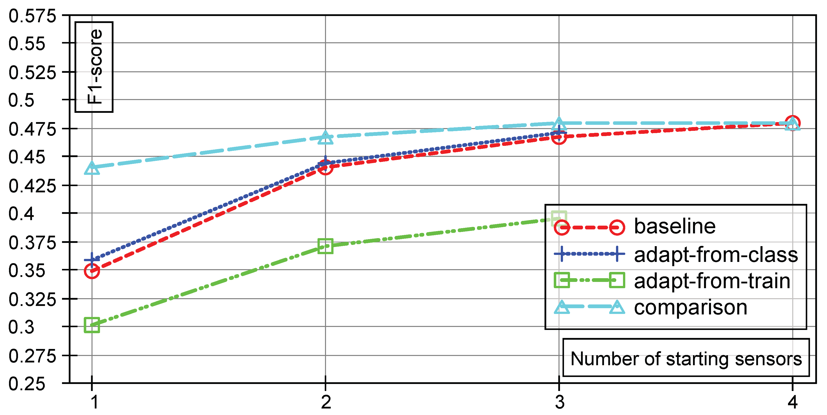
The results of our evaluations are visualized in Figure 3. Baseline and Comparison case are drawn separately, as are the adaptation strategies. The graphs represent the mean F-scores on test data from all of our evaluations.
Two important things can be seen from the graph. First, the fact that the adaptation method that uses labels inferred from the original classifier (adapt-from-class) in average performs better than the baseline case but not as good as the comparison case. The second point is the fact that the adaptation method relying on labels from the original training data (adapt-from-train), i.e., using the backprojected density model, performs significantly worse. The obvious question is why, but the answer can be found when looking closely at the actual projection process. The information from the original d input dimension are kept (mean and covariance matrix values for each component). During marginalization, not only the variance of the additional dimensions is lost, but also the covariance between the d original and the k additional dimensions. This information, however, is integral to the model, i.e., the backprojected model in is not quite as good (with respect to the data), as the model in . Further details are discussed in Section 4.
Table 1 lists the mean F-scores for each sensor combination from testing, along with their standard deviations. It can clearly be seen that the standard deviation for each number of sensors is very low.
This indicates reliable experiment outcomes and only small random influences (if randomness would be dominant to the experiments, the standard deviation would be greater).
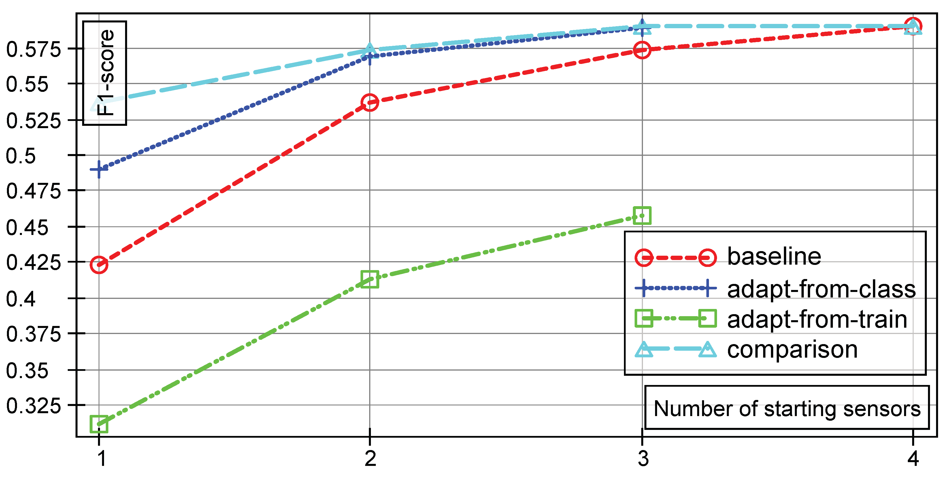
The same effect goes for the training data, with graphs being visualized in Figure 4 and a table with mean and standard deviations shown in Table 2. There again, the standard deviation is very low, i.e., random effects in the experiments are minimal. It is worth noting that, regarding the test data, the models are able to capture the data good enough, to get very close to the comparison case (three sensor case) with a fully autonomous label inference.
4. Discussion
The standard deviations determined by our experiments are very low. We expected higher values, especially as one of the incorporated sensors is a heart rate sensor, which provides far less informative 1D values than, e.g., a 6D IMU that is attached to the dominant hand of a subject. However, a good discrimination of classes was possible on average, as shown by our experiments.
The results presented here are based on a great number of different experiments; however, currently one out of two approaches is performing worse than expected beforehand. The reason for that is clearly the loss of information when marginalizing Gaussian components with arbitrary covariance matrices. Figure 5 visualizes the percentages of marginalized model parameters during backprojection on the x-axis and how often that amount of parameters was neglected by the backprojection on the y-axis.
It can clearly be seen that in more than 50% of all 420 backprojections from the experiments, more than 68% of parameters (describing structural information in the dataset) are neglected. That amount is rather significant, as those parameters describe the structural information in the observed dataset. After the backprojection, the remaining model receives labels in the original input space. The small losses in parameters (9.9% and 14.1% of model parameters lost) only occur when the heart rate sensor was added to the system (and marginalized during backprojection): the extended input space contains 14 dimensions (features), while the original one only contains 12. On the other hand, the worst case is an initial input space based on heart rate data only, so that the addition of one IMU leads to 14 dimensions, but the backprojection goes back to only two dimensions. This hypothesis is supported when looking at the number of parameters that fully describe such models. In d dimensions, a model with components contains
parameters (d entries in the mean vector , entries in the covariance matrix , one mixture coefficient per component and one mixture coefficient is determined by the other J, cf. 2), while in dimensions a model with the same number of components contains
parameters. Taking a look at the difference between Equations (8) and (9) reveals
The loss of information during backprojection thus has a quadratic dependency on the number of added dimensions. As discussed in, e.g., [39], more restrictive forms of covariance matrices (such as diagonal or isotropic matrices) should be investigated. The upside would be less loss of information when projecting from to d dimensions. The downside clearly is a less powerful modeling approach, so the approximating models are expected to have a lower goodness of fit. Furthermore, models gathered so far would be useless, as such restrictions on the covariance matrices will result in totally different models after training.
The approach of backprojecting samples and then using them to train a classifier in however seems very promising. As shown above (adapt-from-class, cf. Figure 3), it works quite well and allows for the autonomous inclusion of new sources in a running classifier during runtime.
In general, it should be possible to create more suitable models if prior knowledge is incorporated into the training process of GMMs in . This is possible by initializing the entries in the mean and covariance matrix with values from an existing model (e.g., the original classifier). The remaining entries can afterwards be filled with, e.g., a GMM that was trained on the new k dimensions only, so that only minor adjustments of and are necessary for each component j. This approach however was not investigated, as the amount of prior knowledge is mostly very small (see above). If that is overcome, another issue is still present: Given the original classifier and a GMM trained on the k new dimensions, how can both be combined into one model and fine-tuned afterwards? Suppose J components in the d dimensional input space (the original classifier) and K components in the k dimensional space, a proper combination would lead to components in dimensions. With all the components in the combined model and all their parameters that need fine tuning, you run into a shortage of training samples extremely quickly, so this approach is not feasible yet.
Outlook
In the future, we plan to expand our investigation on further AR datasets. We are also looking into approaches where the addition of a sensor issues a certain criterion, i.e., selection criteria for available sensors. Besides that, or even in addition to, we are thinking about mechanisms to evaluate several adapted models over time, before switching to one of them. As discussed briefly, another large challenge is the incorporation of prior knowledge, which is available in two different kinds: (1) via the data distribution as modeled by a GMM; and (2) via the class distribution, i.e., available from the training data. Finally, we are considering further research in the combination of generative and discriminative approaches as done by, e.g., Reitmaier et al. [47], who combined the advantages of a discriminative classifier with the data modeling capacities of a generative model using a GMM-based kernel in an SVM.
Author Contributions
M.J. planned, performed and analyzed the experiments, B.S. brought up the topic and contributed the methods. S.T. contributed the state of the art and edited the paper.
Funding
This research was funded by the German research foundation (Deutsche Forschungsgemeinschaft, DFG), grant number [SI 674/12-1].
Acknowledgments
The authors would like to thank the German research foundation (Deutsche Forschungsgemeinschaft, DFG) for the financial support in the context of the “Organic Computing Techniques for Runtime Self-Adaptation of Multi-Modal Activity Recognition Systems” project (SI 674/12-1).
Conflicts of Interest
The authors declare no conflict of interest. The founding sponsors had no role in the design of the study; in the collection, analyses, or interpretation of data; in the writing of the manuscript, and in the decision to publish the results.
References
- Lukowicz, P.; Kirstein, T.; Tröster, G. Wearable systems for health care applications. Methods Inf. Med. 2004, 43, 232–238. [Google Scholar] [PubMed]
- Abowd, G.; Dey, A.; Brown, P.; Davies, N.; Smith, M.; Steggles, P. Towards a better understanding of context and context-awareness. In Proceedings of International Symposium on Handheld and Ubiquitous Computing; Springer: Berlin/Heidelberg, Germany, 1999; pp. 304–307. [Google Scholar]
- Clarkson, B.; Mase, K.; Pentland, A. Recognizing user context via wearable sensors. In Proceedings of the Fourth International Symposium on Wearable Computers, Digest of Papers, Atlanta, GA, USA, 16–17 October 2000; pp. 69–75. [Google Scholar]
- Gellersen, H.; Schmidt, A.; Beigl, M. Multi-sensor context-awareness in mobile devices and smart artifacts. Mob. Netw. Appl. 2002, 7, 341–351. [Google Scholar] [CrossRef]
- Abowd, G.D. Beyond Weiser: From Ubiquitous to Collective Computing. Computer 2016, 49, 17–23. [Google Scholar] [CrossRef]
- Tomforde, S.; Hähner, J.; von Mammen, S.; Gruhl, C.; Sick, B.; Geihs, K. “Know Thyself”-Computational Self-Reflection in Intelligent Technical Systems. In Proceedings of the 2014 IEEE Eighth International Conference on Self-Adaptive and Self-Organizing Systems Workshops, London, UK, 8–12 September 2014; pp. 150–159. [Google Scholar]
- Roggen, D.; Forster, K.; Calatroni, A.; Holleczek, T.; Fang, Y.; Troster, G.; Ferscha, A.; Holzmann, C.; Riener, A.; Lukowicz, P.; et al. OPPORTUNITY: Towards opportunistic activity and context recognition systems. In Proceedings of the 2009 IEEE International Symposium on a World of Wireless, Mobile and Multimedia Networks & Workshops, Kos, Greece, 15–19 June 2009; pp. 1–6. [Google Scholar]
- Pan, S.J.; Yang, Q. A Survey on Transfer Learning. IEEE Trans. Knowl. Data Eng. 2010, 22, 1345–1359. [Google Scholar] [CrossRef] [Green Version]
- Daumé, H, III. Frustratingly Easy Domain Adaptation. arxiv, 2009; arXiv:0907.1815. [Google Scholar]
- Jiang, J. A Literature Survey on Domain Adaptation of Statistical Classifiers. 2008. Available online: http://sifaka.cs.uiuc.edu/jiang4/domainadaptation/survey (accessed on 16 September 2018).
- Duan, L.; Xu, D.; Tsang, I. Learning with Augmented Features for Heterogeneous Domain Adaptation. arXiv, 2012; arXiv:1206.4660v1. [Google Scholar]
- Chen, L.; Hoey, J.; Nugent, C.D.; Cook, D.J.; Yu, Z. Sensor-Based Activity Recognition. IEEE Trans. Syst. Man Cybern. Part C 2012, 42, 790–808. [Google Scholar] [CrossRef]
- Lara, O.D.; Labrador, M.A. A survey on human activity recognition using wearable sensors. Commun. Surv. Tutor. 2013, 15, 1192–1209. [Google Scholar] [CrossRef]
- Bulling, A.; Blanke, U.; Schiele, B. A Tutorial on Human Activity Recognition Using Body-worn Inertial Sensors. ACM Comput. Surv. 2014, 46, 33:1–33:33. [Google Scholar] [CrossRef]
- Shoaib, M.; Bosch, S.; Incel, O.D.; Scholten, H.; Havinga, P.J. Complex Human Activity Recognition Using Smartphone and Wrist-Worn Motion Sensors. Sensors 2016, 16, 426. [Google Scholar] [CrossRef] [PubMed]
- Lane, N.D.; Eisenman, S.B.; Musolesi, M.; Miluzzo, E.; Campbell, A.T. Urban Sensing Systems: Opportunistic or Participatory? In Proceedings of the 9th Workshop on Mobile Computing Systems and Applications, Napa Valley, CA, USA, 25–26 February 2008; pp. 11–16. [Google Scholar]
- Campbell, A.T.; Eisenman, S.B.; Lane, N.D.; Miluzzo, E.; Peterson, R.A. People-centric Urban Sensing. In Proceedings of the 2nd Annual International Workshop on Wireless Internet, Boston, MA, USA, 2–5 August 2006. [Google Scholar]
- Bannach, D.; Sick, B.; Lukowicz, P. Automatic adaptation of mobile activity recognition systems to new sensors. In Proceedings of the 2011 Workshop Mobile Sensing: Challenges, Opportunities, and Future Directions, Beijing, China, 17–21 September 2011. [Google Scholar]
- Bannach, D. Tools and Methods to Support Opportunistic Human Activity Recognition. Ph.D. Thesis, University of Kaiserslautern, Kaiserslautern, Germany, 2015. [Google Scholar]
- Lau, S.; König, I.; David, K.; Parandian, B.; Carius-Düssel, C.; Schultz, M. Supporting patient monitoring using activity recognition with a smartphone. In Proceedings of the 2010 7th International Symposium on Wireless Communication Systems, York, UK, 19–22 September 2010; pp. 810–814. [Google Scholar]
- Turaga, P.; Chellappa, R.; Subrahmanian, V.S.; Udrea, O. Machine Recognition of Human Activities: A Survey. IEEE Trans. Circuits Syst. Video Technol. 2008, 18, 1473–1488. [Google Scholar] [CrossRef] [Green Version]
- Gan, M.T.; Hanmandlu, M.; Tan, A.H. From a Gaussian mixture model to additive fuzzy systems. IEEE Trans. Fuzzy Syst. 2005, 13, 303–316. [Google Scholar] [Green Version]
- Jordan, A. On discriminative vs. generative classifiers: A comparison of logistic regression and naive bayes. Adv. Neural Inf. Process. Syst. 2002, 14, 841. [Google Scholar]
- Raina, R.; Shen, Y.; Mccallum, A.; Ng, A.Y. Classification with hybrid generative/discriminative models. In Advances in Neural Information Processing Systems; MIT Press Ltd.: Cambridge, MA, USA, 2003. [Google Scholar]
- Huỳnh, T.; Schiele, B. Towards Less Supervision in Activity Recognition from Wearable Sensors. In Proceedings of the 2006 10th IEEE International Symposium on Wearable Computers, Montreux, Switzerland, 11–14 October 2006; pp. 3–10. [Google Scholar]
- Kasteren, T.L.M.; Englebienne, G.; Kröse, B.J.A. An activity monitoring system for elderly care using generative and discriminative models. Pers. Ubiquitous Comput. 2010, 14, 489–498. [Google Scholar] [CrossRef] [Green Version]
- Khan, M.A.A.H.; Roy, N.; Hossain, H.M.S. COAR: Collaborative and Opportunistic Human Activity Recognition. In Proceedings of the 2017 13th International Conference on Distributed Computing in Sensor Systems (DCOSS), Ottawa, ON, Canada, 5–7 June 2017; pp. 142–146. [Google Scholar]
- Berger, A.L.; Pietra, V.J.D.; Pietra, S.A.D. A maximum entropy approach to natural language processing. Comput. Linguist. 1996, 22, 39–71. [Google Scholar]
- Villalonga, C.; Pomares, H.; Rojas, I.; Banos, O. Minertial measurement units-Wear: Ontology-based sensor selection for real-world wearable activity recognition. Neurocomputing 2017, 250, 76–100. [Google Scholar] [CrossRef]
- Rokni, S.A.; Ghasemzadeh, H. Autonomous Training of Activity Recognition Algorithms in Mobile Sensors: A Transfer Learning Approach in Context-Invariant Views. IEEE Trans. Mob. Comput. 2018, 17, 1764–1777. [Google Scholar] [CrossRef]
- Munkres, J. Algorithms for the assignment and transportation problems. J. Soc. Ind. Appl. Math. 1957, 5, 32–38. [Google Scholar] [CrossRef]
- Wang, Z.; Wu, D.; Gravina, R.; Fortino, G.; Jiang, Y.; Tang, K. Kernel fusion based extreme learning machine for cross-location activity recognition. Inf. Fusion 2017, 37, 1–9. [Google Scholar] [CrossRef]
- Münzner, S.; Schmidt, P.; Reiss, A.; Hanselmann, M.; Stiefelhagen, R.; Dürichen, R. CNN-based Sensor Fusion Techniques for Multimodal Human Activity Recognition. In Proceedings of the 2017 ACM International Symposium on Wearable Computers, Maui, HI, USA, 11–15 September 2017; pp. 158–165. [Google Scholar]
- Morales, F.J.O.; Roggen, D. Deep convolutional feature transfer across mobile activity recognition domains, sensor modalities and locations. In Proceedings of the 2016 ACM International Symposium on Wearable Computers, Heidelberg, Germany, 12–16 September 2016; pp. 92–99. [Google Scholar]
- Rey, V.F.; Lukowicz, P. Label Propagation: An Unsupervised Similarity Based Method for Integrating New Sensors in Activity Recognition Systems. Proc. ACM Interact. Mob. Wearable Ubiquitous Technol. 2017, 1, 94:1–94:24. [Google Scholar] [CrossRef]
- Jänicke, M.; Sick, B.; Lukowicz, P.; Bannach, D. Self-Adapting Multi-sensor Systems: A Concept for Self-Improvement and Self-Healing Techniques. In Proceedings of the 2014 IEEE Eighth International Conference on the Self-Adaptive and Self-Organizing Systems Workshops (SASOW), London, UK, 8–12 September 2014; pp. 128–136. [Google Scholar]
- Jänicke, M. Self-adapting Multi-Sensor System Using Classifiers Based on Gaussian Mixture Models. In Organic Computing: Doctoral Dissertation Colloquium 2015; Kassel University Press GmbH: Kassel, Germany, 2015; Volume 7, p. 109. [Google Scholar]
- Jänicke, M.; Tomforde, S.; Sick, B. Towards Self-Improving Activity Recognition Systems Based on Probabilistic, Generative Models. In Proceedings of the 2016 IEEE International Conference on Autonomic Computing (ICAC), Würzburg, Germany, 17–22 July 2016; pp. 285–291. [Google Scholar]
- Bishop, C.M. Pattern Recognition and Machine Learning; Springer: New York, NY, USA, 2006. [Google Scholar]
- Reitmaier, T.; Calma, A.; Sick, B. Transductive active learning—A new semi-supervised learning approach based on iteratively refined generative models to capture structure in data. Inf. Sci. 2015, 293, 275–298. [Google Scholar] [CrossRef]
- Duda, R.O.; Hart, P.E.; Stork, D.G. Pattern Classification; John Wiley & Sons: Chichester, NY, USA, 2001. [Google Scholar]
- Fisch, D.; Sick, B. Training of Radial Basis Function Classifiers With Resilient Propagation and Variational Bayesian Inference. In Proceedings of the 2009 International Joint Conference on Neural Networks, Atlanta, GA, USA, 14–19 June 2009; pp. 838–847. [Google Scholar]
- Reiss, A.; Stricker, D. Introducing a New Benchmarked Dataset for Activity Monitoring. In Proceedings of the 2012 16th International Symposium on Wearable Computers, Newcastle, UK, 18–22 June 2012; pp. 108–109. [Google Scholar]
- Reiss, A.; Stricker, D. Creating and benchmarking a new dataset for physical activity monitoring. In Proceedings of the 5th International Conference on Pervasive Technologies Related to Assistive Environments, Heraklion, Crete, Greece, 6–8 June 2012; p. 40. [Google Scholar]
- Lau, S.; David, K. Movement recognition using the accelerometer in smartphones. In Proceedings of the Future Network and Mobile Summit, Florence, Italy, 16–18 June 2010; pp. 1–9. [Google Scholar]
- Sokolova, M.; Japkowicz, N.; Szpakowicz, S. Beyond accuracy, F-score and ROC: A family of discriminant measures for performance evaluation. In Proceedings of Australasian Joint Conference on Artificial Intelligence; Springer: Berlin/Heidelberg, Germany, 2006; pp. 1015–1021. [Google Scholar]
- Reitmaier, T.; Sick, B. The Responsibility Weighted Mahalanobis Kernel for Semi-supervised Training of Support Vector Machines for Classification. Inf. Sci. 2015, 323, 179–198. [Google Scholar] [CrossRef]
Figure 1.
Schematic visualization of classifier adaptation, given a working 1D classifier: Observations in 2D are modeled by a density model (I, top left), which is then backprojected (1) to the original input space (II, top right), where labels are inferred from the 1D training data. (2) This leads to an adapted classifier in the original input space (III, bottom right). The classifier is then forwardprojected (3) to the 2D input space (IV). Crosses are data points, ellipses are height-lines of 2D components. The left column of graphs represents the 2D input space, the right column the original 1D input space.

Figure 2.
Training and test F-scores of the methods investigated by the creators of the PAMAP2 dataset (leftmost five stacks) along with the approach we are pursuing (rightmost stack). The height of the bars represents the mean F-score, the black lines visualize the standard deviations.
Figure 2.
Training and test F-scores of the methods investigated by the creators of the PAMAP2 dataset (leftmost five stacks) along with the approach we are pursuing (rightmost stack). The height of the bars represents the mean F-score, the black lines visualize the standard deviations.

Figure 3.
Test F-scores of the baseline system, the extended system with labels inferred from the training data (adapt-from-train), the extended system with labels inferred from the original classifier (adapt-from-class) and of the comparison system (comparison), for different numbers of starting sensors. In each case, one additional sensor is added to the system.

Figure 4.
Training F-scores with the same notation as in Figure 3. In each case, one additional sensor is added to the system.
Figure 4.
Training F-scores with the same notation as in Figure 3. In each case, one additional sensor is added to the system.

Figure 5.
Percentages of model parameters lost during backprojection.


Table 1.
Mean F-scores on test data for each number of sensor in the form mean ± standard deviation.
Table 1.
Mean F-scores on test data for each number of sensor in the form mean ± standard deviation.
| # Sensors | Method | |||
|---|---|---|---|---|
| Baseline | Adapt-from-Class | Adapt-from-Train | Comparison | |
| 1 | 0.349 ± 0.095 | 0.358 ± 0.078 | 0.302 ± 0.068 | 0.440 ± 0.039 |
| 2 | 0.440 ± 0.039 | 0.444 ± 0.035 | 0.370 ± 0.032 | 0.468 ± 0.027 |
| 3 | 0.468 ± 0.028 | 0.471 ± 0.026 | 0.396 ± 0.021 | 0.480 ± 0.017 |
| 4 | 0.480 ± 0.020 | – | – | 0.480 ± 0.020 |
Table 2.
Mean F-scores on training data for each number of sensor in the form mean ± standard deviation.
Table 2.
Mean F-scores on training data for each number of sensor in the form mean ± standard deviation.
| # Sensors | Method | |||
|---|---|---|---|---|
| Baseline | Adapt-from-Class | Adapt-from-Train | Comparison | |
| 1 | 0.423 ± 0.095 | 0.491 ± 0.080 | 0.311 ± 0.096 | 0.537 ± 0.034 |
| 2 | 0.537 ± 0.035 | 0.569 ± 0.031 | 0.413 ± 0.041 | 0.573 ± 0.023 |
| 3 | 0.573 ± 0.024 | 0.590 ± 0.023 | 0.458 ± 0.023 | 0.591 ± 0.012 |
| 4 | 0.591 ± 0.014 | – | – | 0.591 ± 0.014 |
© 2018 by the authors. Licensee MDPI, Basel, Switzerland. This article is an open access article distributed under the terms and conditions of the Creative Commons Attribution (CC BY) license (http://creativecommons.org/licenses/by/4.0/).
Share and Cite
MDPI and ACS Style
Jänicke, M.; Sick, B.; Tomforde, S. Self-Adaptive Multi-Sensor Activity Recognition Systems Based on Gaussian Mixture Models. Informatics 2018, 5, 38. https://doi.org/10.3390/informatics5030038
AMA Style
Jänicke M, Sick B, Tomforde S. Self-Adaptive Multi-Sensor Activity Recognition Systems Based on Gaussian Mixture Models. Informatics. 2018; 5(3):38. https://doi.org/10.3390/informatics5030038
Chicago/Turabian StyleJänicke, Martin, Bernhard Sick, and Sven Tomforde. 2018. "Self-Adaptive Multi-Sensor Activity Recognition Systems Based on Gaussian Mixture Models" Informatics 5, no. 3: 38. https://doi.org/10.3390/informatics5030038
Note that from the first issue of 2016, this journal uses article numbers instead of page numbers. See further details here.