Penalising Unexplainability in Neural Networks for Predicting Payments per Claim Incurred

Independent Researcher, Level 18, 1 Farrer Place, Sydney, NSW 2000, Australia
Risks 2019, 7(3), 95; https://doi.org/10.3390/risks7030095
Submission received: 13 June 2019
/
Revised: 13 July 2019
/
Accepted: 23 August 2019
/
Published: 1 September 2019
(This article belongs to the Special Issue Claim Models: Granular Forms and Machine Learning Forms)
Abstract
:In actuarial modelling of risk pricing and loss reserving in general insurance, also known as P&C or non-life insurance, there is business value in the predictive power and automation through machine learning. However, interpretability can be critical, especially in explaining to key stakeholders and regulators. We present a granular machine learning model framework to jointly predict loss development and segment risk pricing. Generalising the Payments per Claim Incurred (PPCI) loss reserving method with risk variables and residual neural networks, this combines interpretable linear and sophisticated neural network components so that the ‘unexplainable’ component can be identified and regularised with a separate penalty. The model is tested for a real-life insurance dataset, and generally outperformed PPCI on predicting ultimate loss for sufficient sample size.
1. Introduction
1.1. Rationale
Key business goals for claims models typically include predictive power, automation and ease of use, and interpretability. Predictive power is valuable in any model, but for risk pricing in insurance, higher accuracy leads to selecting lower cost risks and is consequently a competitive advantage. Machine learning and automation improves the business efficiency of the modelling process, and also facilitates models with large numbers of parameters that can reflect complex non-linear relationships. Finally, interpretability is important for communications to business stakeholders and to regulators, particularly in loss reserving to justify projections.
Common actuarial industry practice at the time of writing is for separate sophisticated risk pricing models and relatively simple reserving models. Risk pricing models are typically granular claims models—traditionally Generalised Linear Models (‘GLM’). Increasingly Gradient Boosting Decision Trees/Machines (‘GBM’) have become a popular alternative. Machine learning approaches allow automated identification and fitting of non-linear effects. These can contribute to a higher accuracy than GLM approaches, at the cost of transparency. Conversely, reserving models typically use simple, deterministic triangulation based approaches, with selections based on actuarial judgement. The simplicity of a portfolio approach for loss reserving has the advantages of transparency and the ability to manually adjust selections based on actuarial judgement.
However, separate risk pricing and reserving models can present practical challenges, and results can be circular. In creating risk pricing models, a rescaling adjustment based on reserving is often required to the recent, undeveloped data. In creating reserving models, the pricing view is often used as an initial prior for methods such as Bornhuetter–Ferguson.
Business stakeholders also often demand detailed segmented views on loss ratios to assist in decision-making on underwriting and portfolio management processes, for which a portfolio approach may not be appropriate. Also, where there has been a significant mix shift in the risks insured—perhaps due to growth or shrinkage in particular segments—the portfolio approach breaks down and input from a granular view (often the pricing view) is needed. This suggests that a granular approach to reserving incorporating detailed policy or claims data should be able to model segmented results with better accuracy than simple allocation methods of portfolio Incurred But Not Reported (IBNR) reserves.
1.2. Granular Claims Models
Subsequently, a number of papers have emerged for granular model reserving. An earlier example is a GLM approach, using explanatory variables with conditioning for case estimates (Taylor et al. 2008).
Regularisation via l1 and l2 losses are heavily used as a machine learning technique, both at the portfolio level for loss reserving (Miller and Taylor 2016), or at the granular level to select factors, fit splines or apply other useful constraints to otherwise overparametrised models (Semenovich et al. 2010).
1.3. Neural Networks
Neural network based architectures are extremely flexible and enables use of data in formats such as numerical, categorical, image, time series, and freeform text data. It also allows multiple concurrent outputs using multi-task neural networks (e.g., Fotso 2018; Poon 2018), as well as outputs of a time series using recurrent neural network components such as the gated recurrent unit (Kuo 2018).
However, explainability is an issue when applying this model to claims, as fully connected neural layers can contain large numbers of parameters. Attempts have been made at structuring the network in a more explainable way in other applications, such as constraining neural components to have only a single input and output neuron (Vaughan et al. 2018), or recovering explainability of individual predictions through locally interpretable linear approximations (Ribeiro et al. 2016), but no approach has emerged as an industry standard to date, and it remains unclear whether a fully explainable model structure that preserves the predictive ability of a standard neural network is possible.
1.4. Residual Neural Networks
Residual networks (‘ResNets’) are a type of neural networks originally introduced in vision recognition (He et al. 2015). This allows training of deeper networks for state-of-the-art performance, but has found value in other applications, including actuarial modelling (Schelldorfer and Wuthrich 2019).
ResNets introduce the concept of ‘skip connections’, whereby an earlier layer is directly connected to a later layer (Figure 1). An observation is that for a network with a single residual block, the skip connection is in itself a linear model, ensembled with the neural network layers. With the exponential activation function, the linear model becomes a log-link GLM.
Mathematically, the above residual block in Figure 1b can be expressed as follows:
Let B1, B2, B3 and B4 be weight matrices and a(x) be the activation function. Examples of activation functions include the Rectified Linear Unit (ReLU):
or the Scaled Exponential Linear Unit (SELU), which is used in the model later in this paper:
a(x) = max(0, x)
For a standard feed-forward neural network with two hidden layers, we find b1, b2, b3 and b4 to approximately minimise actual loss versus predicted Loss(, y) where:
x1 = a(B1 xinput),
x2 = a(B2 x1),
However, for the residual network, the skip connection can be added to the output.
1.5. Embeddings
Embeddings are an encoding for categorical variables that is an alternative to one-hot encoding. Each label for a categorical factor is assigned a (typically) 1 × n vector representation that can be trained with the model. For n = 1, each category corresponds with only one value, the embedding can produce results equivalent to one-hot encoding in an additive model structure.
1.6. Hyperparameter Selection
Layers of a neural network can be regularised separately, by applying a different hyperparameter for l1 or l2 regularisation loss to any of the B1, B2, B3 and B4 weights individually as above. For a given loss function Loss(, y), a fully parametrised regularised loss function would be as below (the model in the next section uses mean-squared error loss):
We discuss two approaches for selecting the regularisation parameters. The first is to optimise for holdout loss to find the most predictive model. One method to do so is a Random Grid Search, which tests random sets of hyperparameters and selects the model with the best holdout error, or Bayesian Optimisation, which estimates parameters via a Gaussian Process.
However, a second view is that regularisation provides a mechanism to penalise ‘opaque’ neural features in favour of ‘transparent’ linear features. When the regularisation parameters of the dense layers are set towards high values, the neural network components would shrink towards zero reducing the network to a linear model.
We put forward the concept that between the interpretable linear model and the residual network model, the regularisation parameter for residual network weights represents a continuum of models between those two competing objectives.
Also, by blending the residual model with the original model, we put forward the idea that the weights given to the linear model versus the residual network may potentially form a basis for evaluating the extent to which non-linear effects exist within the data—if the residual model is extremely effective, loss optimisation will bring the blend weight of the residual towards 1.0. Subsequently, the actuary should do additional manual analysis to improve interpretability. An iterative process of feature engineering such as creating splines for age could reduce the need for the opaque neural network component until the neural network is no longer needed.
However, in regards to penalising ‘unexplainability’ through regularising model components, an open question would be in regards to what economic value is to be assigned to interpretability of the model, such that an appropriate penalty can be applied.
With this in mind, we test this approach with a granular model that resembles a fully parametrised PPCI-like model, combining simple linear weights for interpretability with residual components for replicating non-linear effects.
2. Model
2.1. Definitions
Consider a dataset with dates, features, and claims development in the cross-tab format of Table 1:
Features are policy and risk details—rating factors or any details relevant for the risk premium model. This includes origin period, the start dates of triangulation, typically be accident month, quarter or year. Numerical features are normalised to a mean of zero and variance of one, and categorical features are integers encoded for the embeddings.
Exposure weights allow a yearly policy to be divided into multiple monthly records with earned exposure.
Incremental claim count and payments data are matched back to the exposure record and is split into columns by delay period. Delay represents times from accident to the date of claim reporting (counts) or payment with a maximum tail of ‘n’ periods. Per standard actuarial practice, these are ideally adjusted for inflation.
Consequently, the dataset is structured such that
- The sum of ‘claim counts reported by delay’ by origin period is the incremental claims reported triangle,
- The sum of ‘claim payments by delay’ by origin period is the incremental payments triangle,
- If the claim counts and payments were the ultimates, it would be a typical GLM risk pricing dataset.
- The dataset remains reasonably compact as claims are in cross-tab format, which is beneficial from a memory usage perspective.
This allows us to jointly fit a risk pricing and loss reserving model. Let:
- xi be features, for policy exposures i, including the accident or origin period,
- wi,t be exposure weights for exposure i in delay period t, with missing data after the balance date being weighted as 0,
- Ci,t be claim count reported for the exposure in delay period t, with Ci = ΣCi,t and
- Pi,t be claim payments for the exposure in delay period t, with Pi = ΣPi,t.
We wish to build a model for E(Ci,t) and E(Pi,t) based on x and w.
2.2. From Payments Per Claim Incurrred to Granular Model
A traditional PPCI model predicts expected payments P at delay t as a ratio of ultimate incurred C:
where ci is an estimate of ultimate claim count, and qt is the payments per claim incurred.
E(Pi,t) = ci qt,
However, these payments per claim can be factored into the expected claim severity and the percentage paid in each period.
E(Pi,t) = ci q bt, Σtbt = 1.
Consequently, the Payment per Claim Incurred model can be expressed as a simple frequency model (c), a constant claim severity model (q) and a constant percentage paid per period model (b).
In the model, we replace these with granular models for each, which also meets the needs of risk pricing to model frequency and severity by rating factors.
2.3. Network
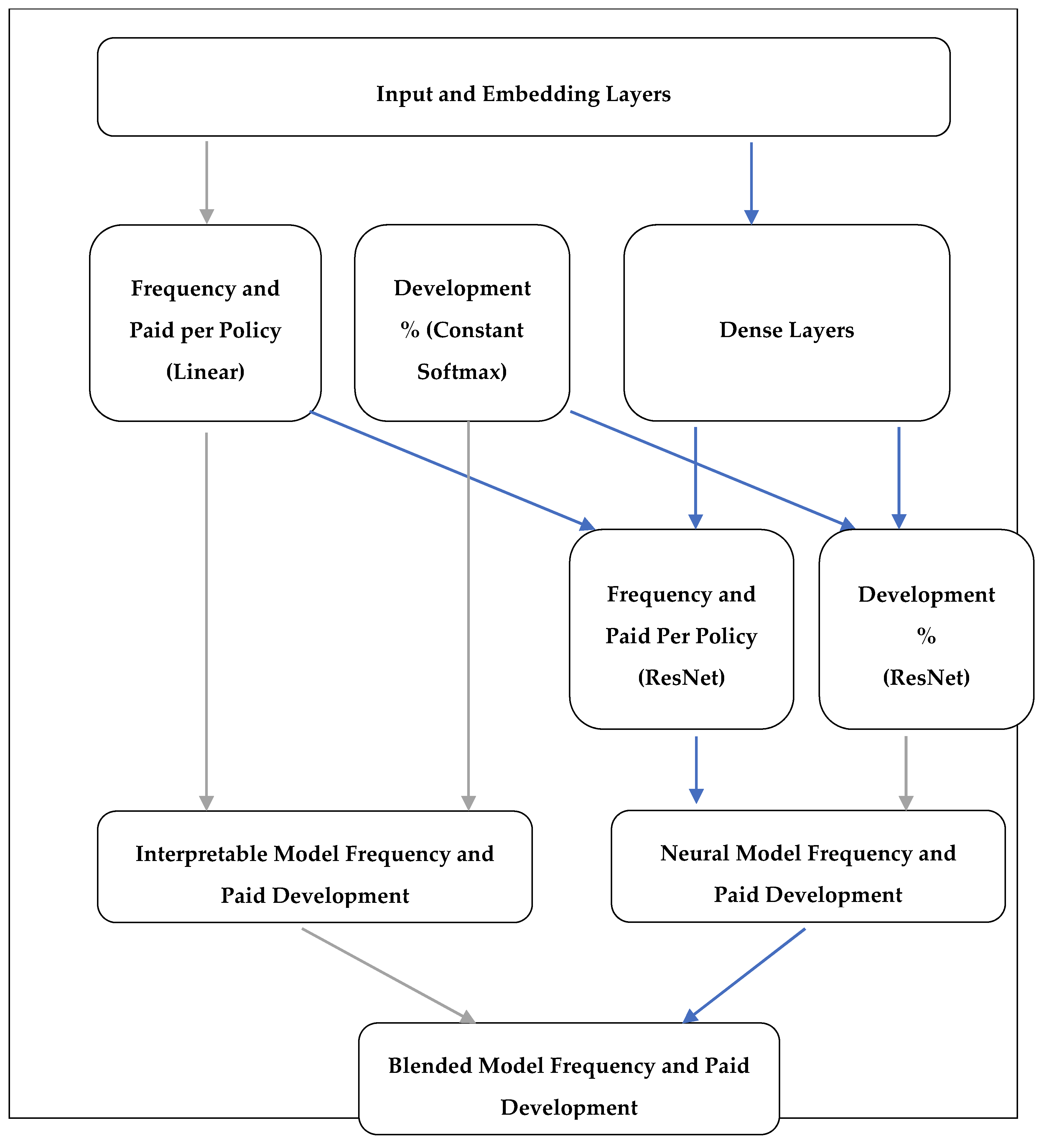
The network diagram is shown in Figure 2.
In the interpretable model, linear models of total frequency and payments per policy were set as a function of the features. With B representing linear weights, let:
clinear = Bc x
With the exponential transform, they become GLMs. The payments per policy can also be set to follow the count logic for a risk premium model with plinear = Bp x or a frequency-severity model by adding the frequency component at each step, such as with plinear = clinear + Bp x.
To allocate that to the prediction of counts and payments at delay t, development parameters dc and dp were fitted with a log-softmax transform, let:
cinterpretable,t = wc,t × exp(c + log(softmax(dc,t))).
The softmax transform enforces that the restriction that the sum of percentage developed is 100%. Without this constraint, it is possible for the expected claim count/paid to ‘explode’ with the percentage developed remaining at low values. In calculations, it is applied as logsoftmax due to numerical stability reasons.
Currently, the development function is fully parametrised but a future potential extension might be to apply a penalty for the percentage-developed distribution or splines to enforce smoothness of the development percentages.
Further parametrising the development network, such as using the xNNs (Vaughan et al.) explainable network splines could reduce the unexplainable components beyond the linear model used.
The ‘neural model’ is similar, except with the residual network components. The proposed network to predict expected frequency and cost per policy is set up with dense layers with outputs concatenated with the original inputs for the final linear model. Three dense layers is often considered to be sufficient for structured data problems but more can be added. For the model results below, SELU activation was used for stability reasons. Consequently, with b representing weight vectors, let:
n1 = SELU(B1 x)
n2 = SELU(B2 n1)
n3 = SELU(B3 n2)
cresidual = B4 n3
dc-residual = B5 n3
cneural, t = wc,t × exp(clinear + cresidual + log_softmax(dc,t))
Finally, a blended model is calculated by fitting a weighted average between the two models, with the weight constrained to be (0, 1) by fitting a parameter wc such that:
Weightc = exp(wc)/(1 + exp(wc)),
cblended,t = Weightc cinterpretable,t + (1 − Weightc cneural,t)
This is intended to provide an indication as to the explanatory power of the residual network compared to the simpler linear model. With optimised hyperparameters, one would expect residual network weights to converge to 1.0 if it always explained better than the linear model.
2.4. Loss
The loss function was set to optimise the sum of mean-squared error loss of all claims count and claims paid per policy for each of the interpretable, residual and blended networks in total, and the additional l1 penalties for the linear risk pricing weights.
One issue with multi-task learning is that if losses are imbalanced, the optimisation may favour one particular set of outputs. While Poisson and Tweedie losses may be more appropriate for counts and payments, respectively, as a simplification, the Mean Squared Error (MSE) (with the exponential activation function) was used for all outputs to avoid having to significantly address this issue. The backpropogated gradients are similar. This may have been insufficient as some results seen later on may have optimised the claims paid, which have higher variation than claims count. More sophisticated approaches would be possible.
2.5. Training: Dropout, Optimiser, Shuffling, Batch Size, and Learn Rate Scheduler
A dropout layer (Srivastava 2014) was applied for training the residual network, and Adam (Kingma and Ba 2015), an adaptive moment estimation optimiser, with separate l2 weight decay penalties for the linear risk pricing and residual network weights, was used as the optimiser for the model. Training data was shuffled to reduce mix bias within each batch. A high batch size was used given the sparsity of the data to ensure sufficient claims data in each batch and gradient norm clipping was applied to improve stability of the training process. Weights initialisation to suitable starting values, learn rate search and the ‘1cycle’ learn rate scheduler (Smith 2018) was used to speed up convergence.
2.6. Language and Package
The model was coded in Python using the Pytorch package. Pytorch was chosen for its high level API compared to Tensorflow, ease of customisation compared to Keras, stability, wide usage and availability of documentation. The version of the code used in this paper was uploaded to: https://github.com/JackyP/penalised-unexplainability-network-payments-per-claim-incurred/blob/1e757249e4f20a75e5e645d5a9f2a7ffb089a8a7/punppci/pytorch.py, with the intention to further develop and, should it reach a state of maturity, to publish in the Python repository PyPI as package ‘punppci’.
3. Dataset Used
3.1. Dataset Details
The model was tested on actual proprietary policy and claim data with 6 features, approximately 250,000 policy exposure records underwritten in 2015–2016 calendar year and 32,000 claims, with claim reported counts and claim paid amounts developed over 24 development months.
For testing accuracy, claims reported or payments transacted after 31 December 2016 was censored for model fitting and used as holdout data.
3.2. Cleaning and Sampling
As part of data preparation, large claims were capped and then both claim frequency and payment was scaled by average frequency and paid per policy of the censored data—an initial estimate of portfolio averages that was free of data leakage from the holdout data. Features were normalised using mean-variance standardisation, with categorical features one-hot encoded for simplicity (although embeddings is recognised to be ideal).
The model was tested on samples of the data of 5000, 10,000, 25,000, 50,000, 100,000 and 200,000 policies with hyperparameters as detailed in Section 4 to test the models’ effectiveness with various dataset sizes, and then on the full dataset with hyperparameter search.
3.3. Comparison with Manual Selections for Chain Ladder and PPCI
The benchmarking is against a mechanical (or naïve) application of chain ladder and PPCI. In practice, factor selections would be based on both actuarial judgement, with manual identification of unusual events, selection of averages where checks for accident or calendar year trends, and manual smoothing of factors.
Consequently, a manual review of the full dataset was also conducted to validate whether there were features that would influence manual selections; however, the triangles were fairly unremarkable given the short duration of the dataset over two accident years, reasonably large size of sample and short tail, non-statutory insurance portfolio. Certain product segments were known to develop slower; however, there was no significant mix shift towards or away from those segments during the period. Individual claim factors also did not appear to have any trends.
4. Results
4.1. Sampling Sizes
For the sampling test, linear l1 and l2 were set to 0.01, the residual network l2 was set to zero for weights and biases. For the full dataset, hyperparameters were firstly grouped into ‘l1 and l2 linear’, ’l2 residual’ and ’l2 bias’, which were applied to both counts and paid for simplicity, and then Bayesian optimisation with the ‘scikit-optimize’ package was applied.
Table 2 shows the comparison of the squared error between actual versus expected ultimates for the model compared with naïve chain ladder and PPCI.
The model outperformed in predicting claim ultimate amounts for 75% of the test cases with policy exposures of 10,000 or over, however, failed to achieve good results for the cases with 5000 policies, due to frequent failing to converge.
However, with neural networks being randomly initialised, there is significant variation in trained model predictions between training runs. We flag model reproducibility and stability as an issue to address for future research into neural based reserving approaches, with the observation that the random initialisations of training weights may lead to variations in the model predictions.
4.2. Bayesian Optimisation of Hyperparameters
The Bayesian optimisation of the hyperparameter set led to penalty factors of l1 and l2 of linear weights being 0.0103, l2 on the bias being 0.0048, and l2 on the dense network of 0.0003. This appears to have led to a good ultimate claim amount prediction, but claim count predictions performing slightly poorer on holdout data.
Although both claim count and claim paid were normalised to means of 1.0 prior to fitting, payments are more variable and consequently contribute a higher proportion of the total squared loss; so it is possible that having the same hyperparameters for both may have led to optimizing the fit of paid while neglecting count.
For the risk pricing applications, Table 3 shows a reasonable lift and also reasonable matching between modelled and actual payments.
This suggests the model is able to correctly distinguish higher and lower risk pricing factors within the portfolio.
With these hyperparameters, the weight attributed to the interpretable model compared to the neural model remained at 71% for claim count and 54% for claim paid, with the lack of weighting of the neural model suggesting that the simpler approach continued to be quite important despite the neural net components.
4.3. Regularisation
Table 4 shows the average absolute value of weights in the dense layers.
A small amount of regularisation appears to be helpful to the fit of the residual model, increasing its weight, but as expected, as weight decay is increased towards higher values, the contribution of the neural network to the blended model diminishes. Due to random initialisation of the network for training, there is some variation in the results.
5. Extending with Freeform Data—Claim Description
There are a number of examples outside actuarial modelling that incorporate unstructured data into neural network models. Typically, this is done by using a pre-trained network for the type of data, such as VG-16G for images, Word2Vec for words, or BERT (Devlin et al. 2018) for sentences. The intermediate outputs of the pre-trained model are used as features for the main model.
However, we are not aware of any academic publications to date applying it within the domain of claims reserving. To demonstrate the earlier claims in Section 1.3, an example would be to extend the model to use freeform text incident descriptions. The incident description for each claim consists of a short phrase manually entered by claims staff describing the claim, e.g., ‘insured damaged phone’. The code is available at: https://gist.github.com/JackyP/99141e403df720a2e752b9bbf08e428c.
The adjustments to the modelling process are as follows: the training dataset consists of the associated incident description and the corresponding subset of the policy-claims data from Section 3 that have had claims. Sentences are tokenised into integer vectors with each vector representing a word. Then, the pre-trained BERT network converts these vectors into an intermediate representation. These are then incorporated as additional features into an expanded model.
6. Conclusions
We extended the use of risk-pricing residual networks to granular reserving applications by introducing a claims development percentage sub-network with a softmax layer to produce a multi-task claim count and paid output, and found it had good performance benchmarked against a traditional PPCI approach when trained on sufficient dataset size.
In regards to interpretability, the softmax layer ensures claims development percentages sum to 100%, and consequently allows separation of risk pricing and claims development effects, whilst also jointly fitting them in a single model. In addition, we also introduced and discussed the concept of separate regularisation between linear and deep effects as a penalty on ‘unexplainability’.
For practical application on large insurance datasets, we tested the use of Adam optimiser with learn rate search, “1cycle” policy optimisation, and setting of reasonable initial bias values. We found this led to effective results, and reasonable training times enabled Bayesian cross-validation optimisation algorithms to be accessible.
To demonstrate the flexible nature of neural networks, the model was also extended with a pre-trained BERT model to use the incident description as a freeform text input for predicting claim payments.
Overall while neural networks techniques for granular loss reserving remains nascent, we anticipate significant opportunities for it to continue developing in the future.
Funding
This research received no external funding.
Conflicts of Interest
The author declares no conflict of interest.
References
- Devlin, Jacob, Ming-Wei Chang, Kenton Lee, and Kristina Toutanova. 2018. BERT: Pre-training of Bidirectional Transformers for Language Understanding. arXiv, arXiv:1810.04805. [Google Scholar]
- Fotso, Stephane. 2018. Deep Neural Networks for Survival Analysis Based on a Multi-Task Framework. arXiv, arXiv:1801.05512v1. [Google Scholar]
- He, Kaiming, Xiangyu Zhang, Shaoqing Ren, and Jian Sun. 2015. Deep Residual Learning for Image Recognition. arXiv, arXiv:1512.03385. [Google Scholar]
- Kingma, Diederik, and Jimmy Ba. 2015. Adam: A Method for Stochastic Optimization. arXiv, arXiv:1412.6980. [Google Scholar]
- Kuo, Kevin. 2018. DeepTriangle: A Deep Learning Approach to Loss Reserving. arXiv, arXiv:1804.09253v3. [Google Scholar]
- Miller, Hugh, Gráinne McGuire, and Greg Taylor. 2016. Self-Assembling Insurance Claim models. Available online: https://actuaries.asn.au/Library/Events/GIS/2016/4dHughMillerSelfassemblingclaimmodels.pdf (accessed on 24 August 2019).
- Poon, Jacky. 2018. Analytics Snippet: Multitasking Risk Pricing Using Deep Learning. Available online: https://www.actuaries.digital/2018/08/23/analytics-snippet-multitasking-risk-pricing-using-deep-learning (accessed on 13 June 2019).
- Ribeiro, Marco Tulio, Sameer Singh, and Carlos Guestrin. 2016. “Why Should I Trust You?”: Explaining the Predictions of Any Classifier. arXiv, arXiv:1602.04938v3. [Google Scholar]
- Schelldorfer, Jürg, and Mario V. Wuthrich. 2019. Nesting Classical Actuarial Models into Neural Networks. Available online: https://ssrn.com/abstract=3320525 (accessed on 22 January 2019).
- Semenovich, Dimitri, Ian Heppell, and Yang Cai. 2010. Convex Models: A New Approach to Common Problems in Premium Rating. Sydney: The Institute of Actuaries of Australia. [Google Scholar]
- Smith, Leslie N. 2018. A disciplined approach to neural network hyper-parameters: Part 1—Learning rate, batch size, momentum, and weight decay. arXiv, arXiv:1803.09820v2. [Google Scholar]
- Srivastava, Nitish, Geoffrey Hinton, Alex Krizhevsky, Ilya Sutskever, and Ruslan Salakhutdinov. 2014. Dropout: A Simple Way to Prevent Neural Networks from Overfitting. The Journal of Machine Learning Research 15: 1929–58. [Google Scholar]
- Taylor, Greg, Gráinne McGuire, and James Sullivan. 2008. Individual claim loss reserving conditioned by case estimates. Annals of Actuarial Science 3: 215–56. [Google Scholar] [CrossRef]
- Vaughan, Joel, Agus Sudjianto, Erind Brahimi, Jie Chen, and Vijayan N. 2018. Nair. Explainable Neural Networks based on Additive Index Models. arXiv, arXiv:1806.01933v1. [Google Scholar]
Figure 1.
(a) A residual block comprising of a group of three layers, showing the skip connection, which can skip one or multiple layers; (b) The same block as a model, showing interpretable linear or GLM model and ‘unexplainable’ neural network.
Figure 1.
(a) A residual block comprising of a group of three layers, showing the skip connection, which can skip one or multiple layers; (b) The same block as a model, showing interpretable linear or GLM model and ‘unexplainable’ neural network.

Figure 2.
Simplified model network graph. Each block represents a group of layers, and the arrows represent the data flow. Grey arrows represent the “interpretable” network flow, whilst blue lines represent the “neural” network flow.
Figure 2.
Simplified model network graph. Each block represents a group of layers, and the arrows represent the data flow. Grey arrows represent the “interpretable” network flow, whilst blue lines represent the “neural” network flow.


Table 1.
Training data format.
| Origin Period | Feature 1 | … | Feature m | Claim Reported by Delay | Claim Paid Reported by Delay | Data Exists Flag by Delay 1 | ||||||
|---|---|---|---|---|---|---|---|---|---|---|---|---|
| x | c | p | w | |||||||||
| 1 | … | n | 1 | … | n | 1 | … | n | ||||
| 1 January 2015 | 1 | 0 | 0 | $2000 | 1 | 1 | ||||||
| 1 December 2016 | - | 0 | NaN | 0 | NaN | 1 | 0 | |||||
| 1 December 2015 | 0 | 1 | 0 | $3000 | 1 | 1 | ||||||
1 Exposure weights if needed would be multiplied to the data existence flag.
Table 2.
Neural network versus traditional chain ladder and PPCI performance (lower is better).
| Test | Sample Size | Seed | Chain Ladder SE Count | PPCI SE Paid | Model SE Count | Model SE Paid | Better Paid SE |
|---|---|---|---|---|---|---|---|
| 0 | 5000 | 1 | 1453.14 | 3436.19 | NaN | NaN | N |
| 1 | 5000 | 2 | 472.17 | 2447.26 | 256.78 | 2183.37 | Y |
| 2 | 5000 | 3 | 431.78 | 5638.29 | NaN | NaN | N |
| 3 | 5000 | 4 | 339.55 | 1652.14 | 224.21 | 3401.45 | N |
| 4 | 5000 | 5 | 1590.66 | 58,388.27 | NaN | NaN | N |
| 5 | 10,000 | 1 | 540.19 | 4070.24 | 823.89 | 5181.73 | N |
| 6 | 10,000 | 2 | 2533.18 | 51,956.42 | 389.81 | 44,884.23 | Y |
| 7 | 10,000 | 3 | 606.79 | 11,418.01 | 272.21 | 7511.17 | Y |
| 8 | 10,000 | 4 | 1810.21 | 209,956.66 | 976.48 | 202,351.99 | Y |
| 9 | 10,000 | 5 | 1057.81 | 52,508.37 | 270.61 | 42,912.06 | Y |
| 10 | 25,000 | 1 | 5575.31 | 35,060.89 | 2583.43 | 23,732.57 | Y |
| 11 | 25,000 | 2 | 4644.56 | 61,120.81 | 750.18 | 51,177.28 | Y |
| 12 | 25,000 | 3 | 1969.43 | 295,767.11 | NaN | NaN | N |
| 13 | 25,000 | 4 | 4054.21 | 309,086.25 | 1985.41 | 299,889.39 | Y |
| 14 | 25,000 | 5 | 1703.19 | 57,953.14 | 1362.94 | 67,186.30 | N |
| 15 | 50,000 | 1 | 25,487.11 | 133,176.94 | 2407.64 | 78,762.94 | Y |
| 16 | 50,000 | 2 | 6313.54 | 125,112.45 | 9515.98 | 116,294.24 | Y |
| 17 | 50,000 | 3 | 3744.60 | 196,970.08 | 6727.98 | 220,488.81 | N |
| 18 | 50,000 | 4 | 13,261.61 | 334,846.96 | 19,096.74 | 284,140.74 | Y |
| 19 | 50,000 | 5 | 4430.90 | 67,546.64 | 1606.70 | 57,256.59 | Y |
| 20 | 100,000 | 1 | 23,441.53 | 312,086.87 | 29,796.32 | 441,193.89 | N |
| 21 | 200,000 | 1 | 64,274.85 | 5,147,858.37 | 28,841.52 | 5,076,289.65 | Y |
| 250,000 with Bayes Opt | 151,959.56 | 1,260,099.15 | 201,002.33 | 961,150.56 | Y | ||
Table 3.
Model versus actual paid segmentation performance—250 k (closer is better).
| Percentile | Model Paid | Actual Paid |
|---|---|---|
| 5% | 0.25 | 0.23 |
| 10.0% | 0.33 | 0.32 |
| 15.0% | 0.47 | 0.47 |
| 20.0% | 0.6 | 0.38 |
| 25.0% | 0.66 | 0.5 |
| 30.0% | 0.71 | 0.54 |
| 35.0% | 0.76 | 0.54 |
| 40.0% | 0.8 | 0.51 |
| 45.0% | 0.85 | 0.6 |
| 50.0% | 0.9 | 0.67 |
| 55.0% | 0.96 | 1.16 |
| 60.0% | 1.02 | 1.24 |
| 65.0% | 1.1 | 1.58 |
| 70.0% | 1.18 | 1.18 |
| 75.0% | 1.28 | 1.17 |
| 80.0% | 1.39 | 0.96 |
| 85.0% | 1.49 | 1.03 |
| 90.0% | 1.62 | 1.8 |
| 95.0% | 1.77 | 2.01 |
| 100.0% | 2.24 | 3.06 |
Table 4.
Average absolute value of weights: dense layers.
| Weight Decay (l2) | Paid w * | Dense Layer 1 | Dense Layer 2 | Dense Layer 3 |
|---|---|---|---|---|
| 0.0001 | 0.97 | 0.043 | 0.026 | 0.031 |
| 0.001 | 2.51 | 0.016 | 0.009 | 0.007 |
| 0.01 | 2.39 | 8.26 × 10⁻⁵ | 1.57 × 10⁻⁵ | 2.71 × 10⁻⁴ |
| 0.1 | 0.64 | 0.004 | 2.36 × 10⁻⁵ | 4.02 × 10⁻⁵ |
* Weighting to residual model is ew/(1 + ew).
© 2019 by the author. Licensee MDPI, Basel, Switzerland. This article is an open access article distributed under the terms and conditions of the Creative Commons Attribution (CC BY) license (http://creativecommons.org/licenses/by/4.0/).
Share and Cite
MDPI and ACS Style
H. L. Poon, J. Penalising Unexplainability in Neural Networks for Predicting Payments per Claim Incurred. Risks 2019, 7, 95. https://doi.org/10.3390/risks7030095
AMA Style
H. L. Poon J. Penalising Unexplainability in Neural Networks for Predicting Payments per Claim Incurred. Risks. 2019; 7(3):95. https://doi.org/10.3390/risks7030095
Chicago/Turabian StyleH. L. Poon, Jacky. 2019. "Penalising Unexplainability in Neural Networks for Predicting Payments per Claim Incurred" Risks 7, no. 3: 95. https://doi.org/10.3390/risks7030095
Note that from the first issue of 2016, this journal uses article numbers instead of page numbers. See further details here.