Optimal Stopping and Utility in a Simple Modelof Unemployment Insurance

Abstract

Managing unemployment is one of the key issues in social policies. Unemployment insurance schemes are designed to cushion the financial and morale blow of loss of job but also to encourage the unemployed to seek new jobs more proactively due to the continuous reduction of benefit payments. In the present paper, a simple model of unemployment insurance is proposed with a focus on optimality of the individual’s entry to the scheme. The corresponding optimal stopping problem is solved, and its similarity and differences with the perpetual American call option are discussed. Beyond a purely financial point of view, we argue that in the actuarial context the optimal decisions should take into account other possible preferences through a suitable utility function. Some examples in this direction are worked out.

1. Introduction

Assessing the risk in financial industries often aims at finding optimal choices in decision-making. In the insurance sector, optimality considerations are crucial primarily for the insurers, who have to address monetary issues (such as how to price the insurance policy so as not to run it at a loss but also to keep the product competitive) and time issues (e.g., when to release the product to the market). Less studied but also important are optimal decisions on behalf of the insured individuals, related to monetary issues (e.g., how profitable is taking up an insurance policy and the right portion of wealth to invest), consumption decisions (e.g., whether to maximize or optimize own consumption), or time-related decisions (such as when it is best to enter or exit an insurance scheme).

In this paper we focus on the particular type of products related to unemployment insurance (UI), whereby an employed individual is covered against the risk of involuntary unemployment (e.g., due to redundancy). Various UI systems are designed to help cushion the financial (as well as morale) blow of loss of job and to encourage unemployed workers to find a new job as early as possible in view of the continued reduction of benefits. The protection is normally provided in the form of regular financial benefits (usually tax free) payable after the insured individual becomes unemployed and until a new job is found, but often only up to a certain maximum duration and with payments gradually decreasing over time. Many countries have UI schemes in place (Holmlund 1998; Kerr 1996), which are often run and funded by the governments, with contributions from employers and workers, but also by private insurance companies (GoCompare 2018). For example, the governmental UI systems administered in France and Belgium in the 1990s provided benefits decreasing with time according to a certain schedule; the amount of the benefit was determined by the age of the worker, their final wage/salary, the number of qualifying years in employment, family circumstances, etc.

In this work we introduce and analyze a simple UI model focusing on the optimal time for the individual to join the scheme. Before setting out the model formally, let us describe the situation in general terms. Consider an individual currently at work but who is concerned about possible loss of job, which may be a genuine potential threat due to the fluidity of the job market and the level of demand in this employment sector. To mitigate this risk, the employer or the social services have an unemployment insurance scheme in place, available to this person (perhaps after a certain qualifying period at work), which upon payment of a one-off entry premium would guarantee to the insured a certain benefit payment proportional to their final wage and determined by a specified declining benefit schedule, until a new job is found (see Figure 1).

The decision the individual is facing is when (rather than if) to join the scheme. What are the considerations being taken into account when contemplating such a decision? On the one hand, delaying the entry may be a good idea in view of the monetary inflation over time—since the entry premium is fixed, its actual value is decreasing with time. Also, it may be reasonably expected that the wage is likely to grow with time (e.g., due to inflation but also as a reward for improved skills and experience), which may have a potential to increase the total future benefit (which depends on the final wage). Last but not least, some savings may be needed before paying the entry premium becomes financially affordable. On the other hand, delaying the decision to join the insurance scheme is risky, as the individual remains unprotected against loss of job, with its financial as well as morale impact.

Thus, there is a scope for optimizing the decision about the entry time—probably not too early but also not too late. Apparently, such a decision should be based on the information available to date, which of course includes the inflation rate and also the unemployment and redeployment rates, all of which should, in principle, be available through the published statistical data. Another crucial input for the decision-making is the individual’s wage as a function of time. We prefer to have the situation where this is modeled as a random process, the values of which may go up as well as down. This is the reason why we do not consider salaries (which are in practice piecewise constant and unlikely to decrease), and instead we are talking about wages, which are more responsive to supply and demand and are also subject to “real-wage” adjustments (e.g., through the consumer price index, CPI). Besides, loss of job is more likely in wage-based employments due to the fluidity of the job market. For simplicity, we model the wage dynamics using a diffusion process called geometric Brownian motion.1

To summarize, the optimization problem for our model aims to maximize the expected net present value of the UI scheme by choosing an optimal entry time ${\tau }^{*}$. We will show that this problem can be solved exactly by using the well-developed optimal stopping theory (Peskir and Shiryaev 2006; Pham 2009; Shiryaev 1999). It turns out that the answer is provided by the hitting time of a suitable threshold $b^{*}$, that is, the first time ${\tau }_{b^{*}}$ when the wage process $X_t$ will reach this level. Since the value of $b^{*}$ is not known in advance, this leads to solving a free-boundary problem for the differential operator (generator) associated with the diffusion process $(X_t)$. In fact, we first conjecture the aforementioned structure of the solution and find the value $b^{*}$, and then verify that this is indeed the true solution to the optimal stopping problem.

In the insurance literature, there has been much interest towards using optimality considerations, including optimal stopping problems. From the standpoint of insurer seeking to maximize their expected returns, the optimal stopping time may be interpreted as the time to suspend the current trading if the situation is unfavorable, and to recalculate premiums; see, e.g., Jensen (1997); Karpowicz and Szajowski (2007); Muciek (2002); and further references therein. Insurance research has also focused on optimality from the individual’s perspective. One important direction relevant to the UI context was the investigation of the job seeking processes, especially when returning from the unemployed status (Boshuizen and Gouweleeuw 1995; McCall 1970; Wang and Wirjanto 2016). This was complemented by a more general research exploring ways to optimize and improve the efficacy of the UI systems (also in terms of reducing government expenditure), using incentives such as a decreasing benefit throughout the unemployment spell, in conjunction with sanctions and workfare; see Fredriksson and Holmlund (2006); Hairault et al. (2007); Hopenhayn and Nicolini (1997); Kolsrud et al. (2018); Landais et al. (2017), to cite but a few. A related strand of research is the study of optimal retirement strategies in the presence of involuntary unemployment risks and borrowing constraints (Choi and Shim 2006; De Angelis and Stabile 2019; Gerrard et al. 2012; Jang and Rhee 2013; Stabile 2006).

To the best of our knowledge, optimal stopping problems in the UI context (such as the optimal entry to/exit from a UI policy) have not received sufficient research attention. This issue is important, because knowing the optimal entry strategies is likely to enhance the motivation for individuals to join the UI scheme, thus ensuring better societal benefits through the UI policies; see analysis and discussion in Rebollo-Sanz and García-Pérez (2015). Knowledge of the optimal entry time for insured individuals, which has impact on the amount and duration of benefits to be claimed, will also help the insurers (both state and private) to optimize their financial practices; see a discussion in Landais and Spinnewijn (2017). Thus, our present work attempts to fill in the gap by addressing the question of the optimal timing to join the UI scheme.

It is interesting to point out that our optimal stopping problem and its solution have a lot in common with (but are not identical to) the well-known American call option in financial mathematics, where the option holder has the right to exercise it at any time (i.e., to buy a certain stock at an agreed price), and the problem is to determine the best time to do that, aiming to maximize the expected financial gain. However, unlike the American call option setting based on purely financial objectives, the optimal stopping solution obtained in our UI model is not entirely satisfactory from the individual’s point of view, because the (optimal) waiting time ${\tau }_{b^{*}}$ may be infinite with positive probability (at least for some values of the parameters), and even if it is finite with probability one, the expected waiting time may be very long.

Motivated by this observation, we argue that certain elements of utility should be added to the analysis, aiming to quantify the individual’s “impatience” as a measure of purpose and satisfaction. We suggest a few simple ideas of how utility might be accommodated in the UI optimal stopping framework. Despite the simplicity of such examples, in most cases they lead to much harder optimal stopping problems. Not attempting to solve these problems in full generality, we confine ourselves to exploring suboptimal solutions in the class of hitting times, which nonetheless provide useful insight into possible effects of inclusion of utility into the optimal stopping context.

The general concept of utility in economics was strongly advocated in the classical book by von Neumann and Morgenstern (1953), whose aim was in particular to overcome the idealistic assumption of a strictly rational behavior of market agents.2 These ideas were quickly adopted in insurance, dating back to Borch (1961), and soon becoming part of the insurance mainstream, culminating in the Expected Utility Theory (see a recent book by Kaas et al. 2008) routinely used as a standard tool to price insurance products. In particular, examples of use of utility in the UI analysis are ubiquitous; see, e.g., Acemoglu and Shimer (2000); Baily (1978); Fredriksson and Holmlund (2006); Hairault et al. (2007); Holmlund (1998); Hopenhayn and Nicolini (1997); Kolsrud et al. (2018); Landais et al. (2017); Landais and Spinnewijn (2017). There have also been efforts to combine optimal stopping and utility (Chen et al. 2019; Choi and Shim 2006; Henderson and Hobson 2008; Karpowicz and Szajowski 2007; Muciek 2002; Wang and Wirjanto 2016). However, all such examples were limited to using utility functions to recalculate wealth, while other important objectives and preferences such as the desire to buy the policy or to reduce the waiting times have not been considered as yet, as far as we can tell.

The rest of the paper is organized as follows. In Section 2, our insurance model is specified and the optimization problem is set up. In Section 3, the optimal stopping problem is solved using a reduction to a suitable free boundary problem, including the identification of the critical threshold $b^{*}$. This is complemented in Section 4 by an elementary derivation using explicit information about the distribution of the hitting times for the geometric Brownian motion. Section 5 addresses various statistical issues and also provides a numerical example illustrating the optimality of the critical threshold $b^{*}$. In Section 6, we carry out the analysis of parametric dependence in our model upon two most significant exogenous parameters, the unemployment rate and the wage drift, and also give an economic interpretation thereof. In Section 7, we make a useful comparison of our problem and its solution with the classical American call option, which leads us to the discussion of the necessity of utility-based considerations in the optimal stopping context. Finally, Section 8 contains the summary discussion of our results, including suggestions for further work. Throughout the paper, we use the standard notation $a\wedge b:=min\{a,b\}$, $a\vee b:=max\{a,b\}$, and $a^{+}:=a\vee 0$.

2. Optimal Stopping Problem

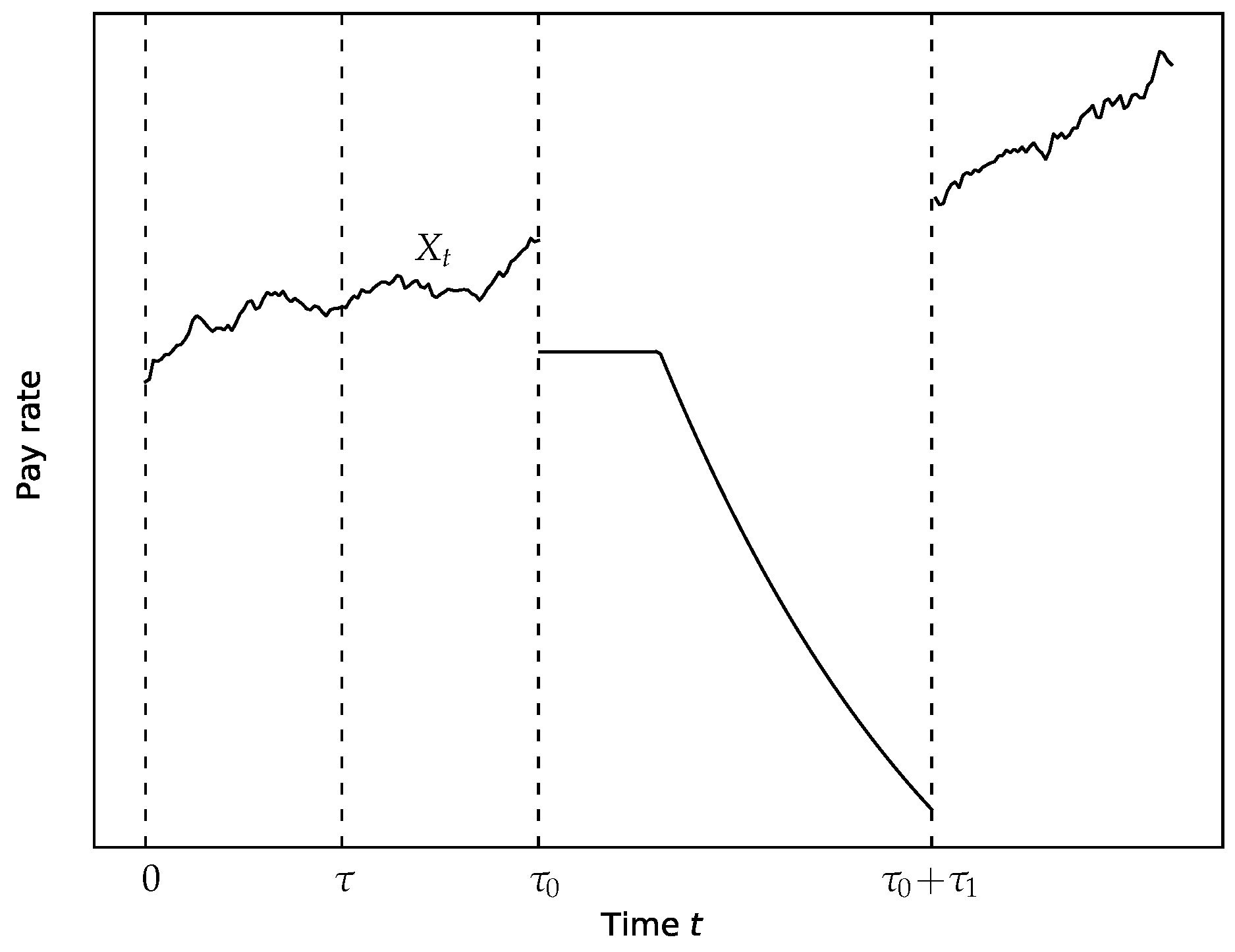
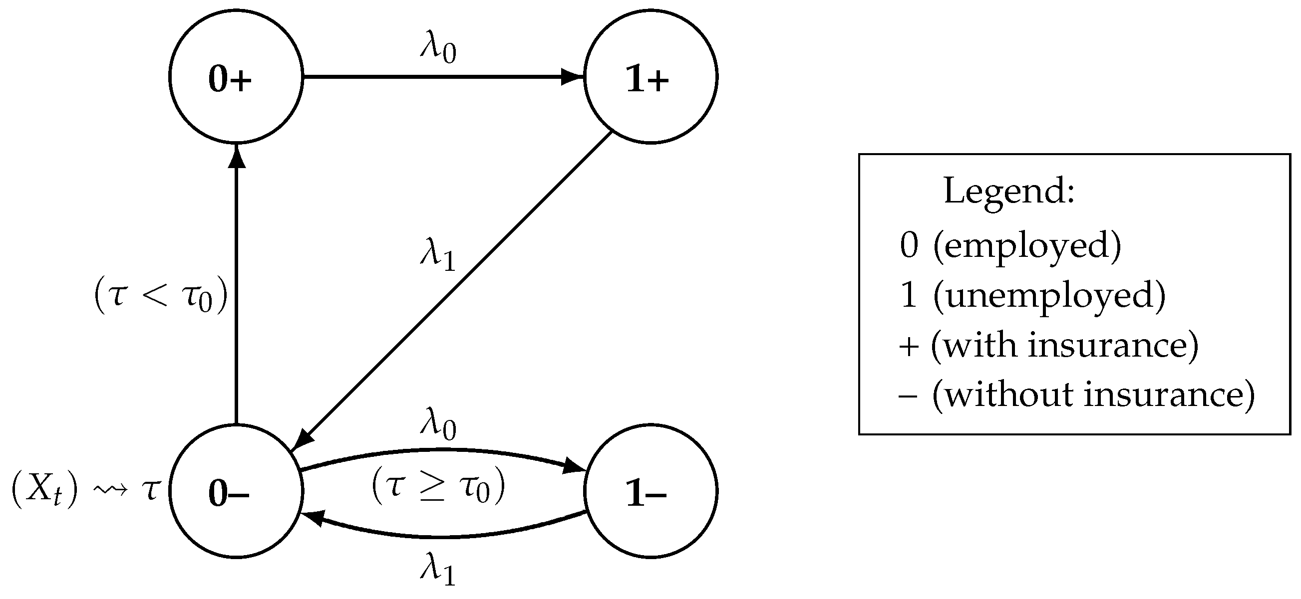
2.1. The Model of Unemployment Insurance

Let us describe our model in more detail. Suppose that time $t\ge 0$ is continuous and is measured (in the units of weeks) starting from the beginning of the individual’s employment. We assume without loss of generality that the unemployment insurance policy is available immediately (although in practice, a qualifying period at work would normally be required for eligibility). Let $X_t>0$ denote the individual’s wage (i.e., payment per week, paid in arrears) as a function of time $t\ge 0$, such that $X_0=x$. We treat $X=(X_t,t\ge 0)$ as a random process defined on a filtered probability space $(\mathsf{\Omega },\mathcal{F},({\mathcal{F}}_t),\mathrm{P})$, where $\mathsf{\Omega }$ is a suitable sample space (e.g., consisting of all possible paths of $(X_t)$), the filtration $({\mathcal{F}}_t)$ is an increasing sequence of $\sigma$-algebras ${\mathcal{F}}_t\subset \mathcal{F}$, and $\mathrm{P}$ is a probability measure on the measurable space $(\mathsf{\Omega },\mathcal{F})$, which determines the distribution of various random inputs in the model, including $(X_t)$. It is assumed that the process $(X_t)$ is adapted to the filtration $({\mathcal{F}}_t)$, that is, $X_t$ is ${\mathcal{F}}_t$-measurable for each $t\ge 0$. Intuitively, ${\mathcal{F}}_t$ is interpreted as the full information available up to time t, and measurability of $X_t$ with respect to ${\mathcal{F}}_t$ means that this information includes knowledge of the values of the process $X_t$.

Furthermore, remembering that $X_t$ is positive valued, we use for it a simple model of geometric Brownian motion driven by the stochastic differential equation

$$\frac{\mathrm{d}{X}_t}{X_t}=\mu \mathrm{d}t+\sigma \mathrm{d}{B}_t,X_0=x,$$

(1)

where $B_t$ is a standard Brownian motion (i.e., with mean zero, $\mathrm{E}(B_t)=0$; variance, $\mathrm{Var}(B_t)=t$; and with continuous sample paths), and $\mu \in \mathbb{R}$ and $\sigma >0$ are the drift and volatility rates, respectively. The Equation (1) is well known to have the explicit solution (Shiryaev 1999, chp. III, §3a, p. 237)

$$X_t=xexp\left\{(\mu -\frac{1}{2}{\sigma }^2)t+\sigma B_t\right\}(t\ge 0).$$

(2)

Note that

$${\mathrm{E}}_x(X_t)=x{\mathrm{e}}^{\mu t},{\mathrm{Var}}_x(X_t)=x^2{\mathrm{e}}^{2\mu t}\left({\mathrm{e}}^{{\sigma }^{2}t}-1\right),$$

(3)

where ${\mathrm{E}}_x$ and ${\mathrm{Var}}_x$ denote expectation and variance with respect to the distribution of $X_t$ given the initial value $X_0=x$.

Let us now specify the unemployment insurance scheme. An individual who is currently employed may join the scheme by paying a fixed one-off premium $P>0$ at the point of entry. If and when the current employment ends (say, at time instant ${\tau }_0$), the benefit proportional to the final wage $X_{{\tau }_0}$ is payable according to the benefit schedule $h(s)$; that is, the payout at time $t\ge {\tau }_0$ is given by $X_{{\tau }_0}h(t-{\tau }_0)$. However, the payment stops when a new job is found after the unemployment spell of duration ${\tau }_1$. For simplicity, we assume that both ${\tau }_0$ and ${\tau }_1$ have exponential distribution (with parameters ${\lambda }_0$ and ${\lambda }_1$, respectively); as mentioned in the Introduction, this guarantees a Markovian nature of the corresponding transitions. These random times are also assumed to be statistically independent of the process $(X_t)$.

Possible transitions in the state space of our insurance model are presented in Figure 2, where symbols “0” and “1” encode the states of being employed and unemployed, respectively, whereas suffixes “+” and “–” indicate whether insurance is in place or not, respectively. Note that all transitions, except from 0– to 0+ (which is subject to optimal control based of observations over the wage process $(X_t)$), occur in a Markovian fashion; that is, the holding times are exponentially distributed (with parameters ${\lambda }_0$ if in states 0– and 0+, or ${\lambda }_1$ if in states 1– and 1+).

The individual’s decision about a suitable time to join the scheme is based on the information available to date. In our model, this information encoded in the filtration $({\mathcal{F}}_t)$ is provided by ongoing observations over the wage process $(X_t)$. Thus, admissible strategies for choosing $\tau$ must be adapted to the filtration $({\mathcal{F}}_t)$; namely, at any time instant, $t\ge 0$, it should be possible to determine whether $\tau$ has occurred or not yet, given all the information in ${\mathcal{F}}_t$. In mathematical terms, this means that $\tau$ is a stopping time, whereby for any $t\ge 0$ the event $\{\tau >t\}$ belongs to the $\sigma$-algebra ${\mathcal{F}}_t$ (see, e.g., Yeh 1995, chp.1, §3, p. 25).

Remark 1.

In general, a stopping time τ is allowed to take values in $[0,\infty ]$ including ∞, in which case waiting continues indefinitely and the decision to join the scheme is never taken. In practice, it is desirable that the stopping time τ be finite almost surely (a.s.) (i.e., ${\mathrm{P}}_x(\tau <\infty )=1$), but this may not always be the case (see Section 4.1).

2.2. Setting the Optimal Stopping Problem

As was explained informally in the introduction, there is a scope for optimizing the choice of the entry time $\tau$, where optimality is measured by maximizing the expected financial gain from the scheme. Our next goal is to obtain an expression for the expected gain under the contract. First of all, conditional on the final wage $X_{{\tau }_0}$, the expected future benefit to be received under this insurance contract is given by

$$X_{{\tau }_0}\mathrm{E}\left({\int }_0^{{\tau }_1}{\mathrm{e}}^{-rs}h(s)\mathrm{d}s\right)=\beta X_{{\tau }_0},$$

(4)

where r is the inflation rate and

$$\beta :={\int }_0^{\infty }{\lambda }_1{\mathrm{e}}^{-{\lambda }_{1}t}H(t)\mathrm{d}t,H(t):={\int }_0^t{\mathrm{e}}^{-rs}h(s)\mathrm{d}s.$$

(5)

Note that the expectation in formula (4) is taken with respect to the (exponential) random waiting time ${\tau }_1$ (with parameter ${\lambda }_1$), and that the expression inside integration involves discounting to the beginning of unemployment at time ${\tau }_0$.

Example 1.

A specific example of the benefit schedule $h(s)$ is as follows,

$$h(s)=\left\{\begin{array}{cc}{h}_0,\hfill & 0\le s\le s_0,\hfill \\ h_0{\mathrm{e}}^{-\delta (s-s_0)},\hfill & s\ge s_0,\hfill \end{array}\right.$$

(6)

where $0<h_0\le 1$, $0\le s_0\le \infty$, and $\delta >0$. Thus, the insured receives a certain fraction of their final wage (i.e., $h_0{X}_{{\tau }_0}$) for a grace period $s_0$, after which the benefit is falling down exponentially with rate δ. This example is motivated by the declining unemployment compensation system in France (Kerr 1996).3 Having specified the schedule function, all calculations can be done explicitly. In particular, the constant β in (4) is calculated from (5) as

$$\beta =\frac{h_0\left(1-{\mathrm{e}}^{-(r+{\lambda }_1)s_0}\right)}{r+{\lambda }_1}+\frac{h_0{\mathrm{e}}^{-(r+{\lambda }_1)s_0}}{r+{\lambda }_1+\delta }.$$

In the extreme cases $s_0=0$ or $s_0=\infty$, this expression simplifies to

$$\beta =\left\{\begin{array}{cc}{\displaystyle \frac{h_0}{{\lambda }_1}\left(1-\frac{r+\delta }{r+{\lambda }_1+\delta }\right),}\hfill & s_0=0,\hfill \\ {\displaystyle \frac{h_0}{{\lambda }_1}\left(1-\frac{r}{r+{\lambda }_1}\right),}\hfill & s_0=\infty .\hfill \end{array}\right.$$

Here, the first factor has a clear meaning as the product of pay per week ($h_0$) and the mean duration of the benefit payment ($\mathrm{E}({\tau }_1)=1/{\lambda }_1$), whereas the second factor takes into account the discounting at rates r and δ.

Returning to the general case, if the contract is entered immediately (subject to the payment of premium P), then the net expected benefit discounted to the entry time $t=0$ is given by the gain function

$$g(x):={\mathrm{E}}_x\left({\mathrm{e}}^{-r{\tau }_0}\beta X_{{\tau }_0}\right)-P,$$

(7)

where $x=X_0$ is the starting wage and the symbol ${\mathrm{E}}_x$ now indicates expectation with respect to both ${\tau }_0$ and $X_{{\tau }_0}$. Recall that the random time ${\tau }_0$ is independent of the process $(X_t)$ and has the exponential distribution with parameter ${\lambda }_0$. Using the total expectation formula (Shiryaev 1996, §II.7, Definition 3, p. 214, and Property G*, p. 216) and substituting the expression (3), the expectation in (7) is computed as follows,

$$\begin{array}{cc}\hfill {\mathrm{E}}_x\left({\mathrm{e}}^{-r{\tau }_0}{X}_{{\tau }_0}\right)& ={\displaystyle {\mathrm{E}}_x\left({\mathrm{e}}^{-r{\tau }_0}{\mathrm{E}}_x(X_{{\tau }_0}|{\tau }_0)\right)}\hfill \\ \hfill & ={\mathrm{E}}_x\left({\mathrm{e}}^{-r{\tau }_0}(x{\mathrm{e}}^{\mu {\tau }_0})\right)=x{\int }_0^{\infty }{\mathrm{e}}^{(\mu -r)t}{\lambda }_0{\mathrm{e}}^{-{\lambda }_{0}t}\mathrm{d}t\hfill \\ \hfill & \hspace{1em}\hspace{1em}\hspace{1em}\hspace{1em}\hspace{1em}\hspace{1em}\hspace{1em}\hspace{1em}\hspace{1em}=\frac{{\lambda }_{0}x}{r+{\lambda }_0-\mu }.\hfill \end{array}$$

(8)

Thus, substituting (8) into (7) and denoting

$$\tilde{r}:=r+{\lambda }_0,{\beta }_1:=\frac{\beta {\lambda }_0}{\tilde{r}-\mu },$$

(9)

the gain function is represented explicitly as

$$g(x)={\beta }_{1}x-P.$$

(10)

Of course, the computation in (8) is only meaningful as long as

$$\mu <r+{\lambda }_0=\tilde{r}.$$

(11)

Assumption 1.

In what follows, we always assume that the condition (11) is satisfied.

Remark 2.

In real-life applications, the wage growth rate μ is rather small (but may be either positive or negative). It is unlikely to exceed the inflation rate r, but even if it does, then it is hardly possible economically that it is greater than the combined inflation–unemployment rate $\tilde{r}=r+{\lambda }_0$. Thus, the condition (11) is absolutely realistic.

To generalize the expression (10), consider a delayed entry time $\tau >0$ (tacitly assuming that $\tau <\infty$). Discounting first to the entry time $\tau$ when the deduction of the premium P is activated, and then further down to the initial time moment $t=0$, yields the expected net present value of the total gain as a function of the initial wage x,

$$\mathrm{e}\mathrm{NPV}(x;\tau ):={\mathrm{E}}_x\left[{\mathrm{e}}^{-r\tau }\left({\mathrm{e}}^{-r({\tau }_0-\tau )}\beta X_{{\tau }_0}-P\right){\mathrm{𝟙}}_{\{\tau <{\tau }_0\}}\right],$$

(12)

where the expectation on the right now also includes averaging with respect to $\tau$, which is a functional of the path $(X_t)$. Note that the indicator function under the expectation specifies that the entry time $\tau$ must occur prior to ${\tau }_0$, for otherwise there will be no gain.

Remark 3.

The notation (12) emphasizes that the expected net present value depends on the specific entry time τ. As was intuitively explained in the Introduction, there is a scope for optimizing the choice of τ, where optimality is measured by maximizing $\mathrm{e}\mathrm{NPV}(x;\tau )$.

Formula (12) indicates that the decision time $\tau$ has a finite (random) expiry date ${\tau }_0$ (using the terminology of financial options). However, the expectation in (12) involves averaging with respect to ${\tau }_0$. Moreover, taking advantage of exponential distribution of ${\tau }_0$, the expression (12) can be rewritten without any expiry date (i.e., as a perpetual option).

Lemma 1.

The expected net present value defined by formula (12) can be expressed in the form

$$\mathrm{e}\mathrm{NPV}(x;\tau )={\mathrm{E}}_x\left[{\mathrm{e}}^{-\tilde{r}\tau }g(X_{\tau }){\mathrm{𝟙}}_{\{\tau <\infty \}}\right],$$

(13)

where the function $g(·)$ is defined in (7) and $\tilde{r}=r+{\lambda }_0$ (see (9)).

Proof. 

Since the distribution of ${\tau }_0$ is exponential, the excess time ${\tilde{\tau }}_0:={\tau }_0-\tau$ conditioned on $\{\tau <{\tau }_0\}$ is again exponentially distributed (with the same parameter ${\lambda }_0$) and independent of $\tau$. Hence, conditioning on $\tau$ (restricted to the event $\{\tau <\infty \}$) and using the total expectation formula as before, together with the (strong) Markov property of the process $(X_t)$, we get from (12)

$$\begin{array}{cc}\hfill \mathrm{e}\mathrm{NPV}(x;\tau )& ={\mathrm{E}}_x\left({\mathrm{E}}_x\left[{\mathrm{e}}^{-r\tau }({\mathrm{e}}^{-r({\tau }_0-\tau )}\beta X_{{\tau }_0}-P){\mathrm{𝟙}}_{\{{\tau }_0>\tau \}}\right|\tau ]\right)\hfill \\ \hfill & ={\mathrm{E}}_x\left({\mathrm{e}}^{-r\tau }{\mathrm{E}}_x\left[({\mathrm{e}}^{-r{\tilde{\tau }}_0}\beta X_{\tau +{\tilde{\tau }}_0}-P)|\tau \right]·{\mathrm{E}}_x({\mathrm{𝟙}}_{\{{\tau }_0>\tau \}}\left|\tau \right)\right)\hfill \\ \hfill & ={\mathrm{E}}_x\left({\mathrm{e}}^{-r\tau }{\mathrm{E}}_{X_{\tau }}({\mathrm{e}}^{-r{\tilde{\tau }}_0}\beta {\tilde{X}}_{{\tilde{\tau }}_0}-P)·{\mathrm{P}}_x({\tau }_0>\tau |\tau )\right),\hfill \end{array}$$

(14)

where ${\tilde{X}}_t:=X_{\tau +t}$ ($t\ge 0$) is a shifted wage process starting at ${\tilde{X}}_0=X_{\tau }$. Substituting ${\mathrm{P}}_x({\tau }_0>\tau |\tau )={\mathrm{e}}^{-{\lambda }_0\tau }$ and recalling notation (7), formula (14) is reduced to (13). □

Finally, without loss we can remove the indicator from the expression (13) by defining the value of the random variable under expectation to be zero on the event $\{\tau =\infty \}$. This definition is consistent with the limit at infinity. Indeed, observe using (2) and (8) that

$$\begin{array}{cc}\hfill {\mathrm{e}}^{-\tilde{r}t}g(X_t)& ={\mathrm{e}}^{-\tilde{r}t}\left({\beta }_{1}x{\mathrm{e}}^{(\mu -{\sigma }^2/2)t+\sigma B_t}-P\right)\hfill \\ \hfill & ={\beta }_{1}xexp\left\{-t(\tilde{r}-\mu +\frac{1}{2}{\sigma }^2+\sigma t^{-1}{B}_t)\right\}-P{\mathrm{e}}^{-\tilde{r}t}.\hfill \end{array}$$

(15)

Due to the condition (11), $\tilde{r}-\mu +\frac{1}{2}{\sigma }^2>\frac{1}{2}{\sigma }^2>0$. In addition, by the (strong) law of large numbers for the Brownian motion (see, e.g., Durrett 1999, Exercise 6.4, p. 265, or Shiryaev 1999, chp. III, §3b, p. 246),

$$\underset{t\to \infty }{lim}{t}^{-1}{B}_t=0(\mathrm{P}-\mathrm{a}.\mathrm{s}.).$$

Thus, the limit of (15) as $t\to \infty$ is zero (${\mathrm{P}}_x$-a.s.). Hence, the event $\{\tau =\infty \}$ does not contribute to the expectation (13), so that, substituting (8), we get

$$\mathrm{e}\mathrm{NPV}(x;\tau )={\mathrm{E}}_x\left({\mathrm{e}}^{-\tilde{r}\tau }g(X_{\tau })\right).$$

(16)

To summarize, identification of the optimal entry time $\tau ={\tau }^{*}$, in the sense of maximizing the expected net present value $\mathrm{e}\mathrm{NPV}(x;\tau )$ as a function of strategy $\tau$ (see (16)), is reduced to solving the following optimal stopping problem,

$$v(x)=\underset{\tau }{sup}{\mathrm{E}}_x\left({\mathrm{e}}^{-\tilde{r}\tau }g(X_{\tau })\right),$$

(17)

where the function $g(x)$ is given by (10) and the supremum is taken over the class of all admissible stopping times $\tau$ (i.e., adapted to the filtration $({\mathcal{F}}_t)$). The supremum $v(x)$ in (17) is called the value function of the optimal stopping problem.

2.3. Allowing for Mortality

The simple model of unemployment insurance set out in Section 2.1 can be easily extended to include mortality. Following (Merton 1971, pp. 399–401), suppose that the individual who contemplates taking out the unemployment insurance policy may die (say, at a random time ${\tau }_2$ from zero), independently of employment-related events and subject to a constant force of mortality ${\lambda }_2$. That is to say, given that the individual is alive at current age $t\ge 0$, the residual lifetime ${\tau }_2-t$ is an independent random variable exponentially distributed with parameter ${\lambda }_2$,

$$\mathrm{P}\left({\tau }_2-t>s|{\tau }_2>t\right)={\mathrm{e}}^{-{\lambda }_{2}s}(s\ge 0).$$

The necessary modifications to the unemployment insurance model of Section 2.2 start by adjusting the formula for the expected future benefit (see (4)). Assuming that death does not occur prior to the time ${\tau }_0$ of losing the job (i.e., ${\tau }_2>{\tau }_0$, so that ${\tilde{\tau }}_2:={\tau }_2-{\tau }_0$ is exponentially distributed with parameter ${\lambda }_2$), the benefit payments cease at ${\tau }_1\wedge {\tilde{\tau }}_2$ (i.e., when a new job is found or at death, whichever occurs first). Since ${\tau }_1$ and ${\tilde{\tau }}_2$ are independent and both have exponential distributions, the random variable ${\tau }_1\wedge {\tilde{\tau }}_2$ has the exponential distribution with parameter ${\lambda }_1+{\lambda }_2$. Hence, the constant $\beta$ from (5) is now written as

$$\beta ={\int }_0^{\infty }({\lambda }_1+{\lambda }_2){\mathrm{e}}^{-({\lambda }_1+{\lambda }_2)t}H(t)\mathrm{d}t.$$

Next, we need to take into account the effect of death in service, that is, if ${\tau }_2\le {\tau }_0$. To be specific, it is reasonable to assume that the lump sum to be paid by the employer in this case is proportional to the final wage, say $a^{†}{X}_{{\tau }_2}$. Then, separating the cases where death occurs after or prior to loss of job, it is easy to see that the definition (7) of the gain function (i.e., net expected benefit discounted to the policy entry time) takes the form

$$g(x)={\mathrm{E}}_x\left({\mathrm{e}}^{-r{\tau }_0}\beta X_{{\tau }_0}{\mathrm{𝟙}}_{\{{\tau }_0<{\tau }_2\}}\right)+{\mathrm{E}}_x\left({\mathrm{e}}^{-r{\tau }_0}{a}^{†}{X}_{{\tau }_2}{\mathrm{𝟙}}_{\{{\tau }_2\le {\tau }_0\}}\right)-P.$$

(18)

The first expectation in (18) is computed using conditioning on ${\tau }_0$ and the total expectation formula (cf. (8)),

$$\begin{array}{cc}\hfill {\mathrm{E}}_x\left({\mathrm{e}}^{-r{\tau }_0}{X}_{{\tau }_0}{\mathrm{𝟙}}_{\{{\tau }_0<{\tau }_2\}}\right)& ={\displaystyle {\mathrm{E}}_x\left[{\mathrm{e}}^{-r{\tau }_0}{\mathrm{E}}_x\left(X_{{\tau }_0}{\mathrm{𝟙}}_{\{{\tau }_0<{\tau }_2\}}|{\tau }_0\right)\right]}\hfill \\ \hfill & ={\displaystyle {\mathrm{E}}_x\left[{\mathrm{e}}^{-r{\tau }_0}{\mathrm{E}}_x(X_{{\tau }_0}|{\tau }_0)·{\mathrm{P}}_x({\tau }_2>{\tau }_0|{\tau }_0)\right]}\hfill \\ \hfill & ={\mathrm{E}}_x\left({\mathrm{e}}^{-r{\tau }_0}x{\mathrm{e}}^{\mu {\tau }_0}{\mathrm{e}}^{-{\lambda }_2{\tau }_0}\right)=x{\int }_0^{\infty }{\mathrm{e}}^{(\mu -r-{\lambda }_2)t}{\lambda }_0{\mathrm{e}}^{-{\lambda }_{0}t}\mathrm{d}t\hfill \\ \hfill & \hspace{1em}\hspace{1em}\hspace{1em}\hspace{1em}\hspace{1em}\hspace{1em}\hspace{1em}\hspace{1em}\hspace{1em}\hspace{1em}=\frac{{\lambda }_{0}x}{r+{\lambda }_0+{\lambda }_2-\mu },\hfill \end{array}$$

(19)

where in the second line we used conditional independence of $X_{{\tau }_0}$ and ${\tau }_2$ given ${\tau }_0$. Similarly, by conditioning on ${\tau }_2$ the second expectation in (18) is represented as

$$\begin{array}{cc}\hfill {\mathrm{E}}_x\left({\mathrm{e}}^{-r{\tau }_0}{X}_{{\tau }_2}{\mathrm{𝟙}}_{\{{\tau }_2\le {\tau }_0\}}\right)& ={\mathrm{E}}_x\left[X_{{\tau }_2}{\mathrm{E}}_x\left({\mathrm{e}}^{-r{\tau }_0}{\mathrm{𝟙}}_{\{{\tau }_0\ge {\tau }_2\}}|{\tau }_2\right)\right]\hfill \\ \hfill & ={\mathrm{E}}_x\left[X_{{\tau }_2}{\int }_{{\tau }_2}^{\infty }{\mathrm{e}}^{-rt}{\lambda }_0{\mathrm{e}}^{-{\lambda }_{0}t}\mathrm{d}t\right]\hfill \\ \hfill & =\frac{{\lambda }_0}{r+{\lambda }_0}{\mathrm{E}}_x\left(X_{{\tau }_2}{\mathrm{e}}^{-(r+{\lambda }_0){\tau }_2}\right).\hfill \end{array}$$

(20)

Again conditioning on ${\tau }_2$, the last expectation is computed as follows,

$$\begin{array}{cc}\hfill {\mathrm{E}}_x\left(X_{{\tau }_2}{\mathrm{e}}^{-(r+{\lambda }_0){\tau }_2}\right)& ={\mathrm{E}}_x\left[{\mathrm{e}}^{-(r+{\lambda }_0){\tau }_2}{\mathrm{E}}_x(X_{{\tau }_2}|{\tau }_2)\right]\hfill \\ \hfill & ={\mathrm{E}}_x\left({\mathrm{e}}^{-(r+{\lambda }_0){\tau }_2}x{\mathrm{e}}^{\mu {\tau }_2}\right)\hfill \\ \hfill & =x{\int }_0^{\infty }{\mathrm{e}}^{-(r+{\lambda }_0-\mu )t}{\lambda }_2{\mathrm{e}}^{-{\lambda }_{2}t}\mathrm{d}t\hfill \\ \hfill & =\frac{{\lambda }_{2}x}{r+{\lambda }_0+{\lambda }_2-\mu }.\hfill \end{array}$$

(21)

Finally, substituting the expressions (19)–(21) into the definition (18), we obtain explicitly

$$g(x)=\frac{{\lambda }_{0}x}{r+{\lambda }_0+{\lambda }_2-\mu }\left(\beta +\frac{{\lambda }_2{a}^{†}}{r+{\lambda }_0}\right)-P.$$

This expression has the same form as (10) but with the parameters $\tilde{r}$ and ${\beta }_1$ redefined as follows (cf. (9)),

$$\tilde{r}:=r+{\lambda }_0+{\lambda }_2,{\beta }_1:=\frac{{\lambda }_0}{\tilde{r}-\mu }\left(\beta +\frac{{\lambda }_2{a}^{†}}{r+{\lambda }_0}\right).$$

In addition, the inequality (11) of Assumption 1 is updated accordingly. Subject to this reparameterization, all subsequent calculations leading to the optimal stopping problem (17) remain unchanged.

For the sake of clarity and in order not to distract the reader by unnecessary technicalities, in the rest of the paper we adhere to the original version of the model (i.e., with no mortality, ${\lambda }_2=0$); however, see the discussion at the end of Section 6.4 indicating an important regularizing role of mortality, helping to avoid undesirable inconsistencies of the model at small unemployment rates ${\lambda }_0$.

2.4. A Priori Properties of the Value Function

The next lemma shows that the optimal stopping problem (17) is well posed.

Lemma 2.

The value function $x\mapsto v(x)$ of the optimal stopping problem (17) has the following properties:

(i)

$v(0)=0$ and, moreover, $v(x)\ge 0$ for all $x\ge 0$;

(ii)

$v(x)<\infty$ for all $x\ge 0$.

Proof. 

(i) If $x=0$ then, due to (2), $X_t\equiv 0$ (${\mathrm{P}}_0$-a.s.) and the stopping problem (17) is reduced to

$$v(0)=\underset{\tau }{sup}{\mathrm{E}}_0(-P{\mathrm{e}}^{-\tilde{r}\tau }),$$

which has the obvious solution $\tau =\infty$ (${\mathrm{P}}_0$-a.s.), with the corresponding supremum value $v(0)=0$. Furthermore, by considering $\tau =\infty$ (${\mathrm{P}}_x$-a.s.) it readily follows from (17) that $v(x)\ge 0$ for all $x\ge 0$.

(ii) Recalling that $\mu <\tilde{r}$ (see Assumption 1), observe that the process ${\mathrm{e}}^{-\tilde{r}t}{X}_t$ is a supermartingale; indeed, for $0\le s\le t$ we have, using (2) and (3),

$$\begin{array}{cc}\hfill {\mathrm{E}}_x({\mathrm{e}}^{-\tilde{r}t}{X}_t|{\mathcal{F}}_s)& ={\mathrm{e}}^{-\tilde{r}t}{X}_s\mathrm{E}\left({\mathrm{e}}^{\sigma (B_t-B_s)+(\mu -\frac{1}{2}{\sigma }^2)(t-s)}\right)\hfill \\ \hfill & ={\mathrm{e}}^{-\tilde{r}t}{X}_s{\mathrm{e}}^{\mu (t-s)}\le {\mathrm{e}}^{-\tilde{r}s}{X}_s({\mathrm{P}}_x-\mathrm{a}.\mathrm{s}.).\hfill \end{array}$$

In particular,

$${\mathrm{E}}_x({\mathrm{e}}^{-\tilde{r}t}{X}_t)\le {\mathrm{E}}_x(X_0)=x.$$

Hence, by Doob’s optional sampling theorem for non-negative, right-continuous supermartingales (Yeh 1995, Theorem 8.18, pp. 140–41), we have

$${\mathrm{E}}_x({\mathrm{e}}^{-\tilde{r}\tau }{X}_{\tau })\le {\mathrm{E}}_x(X_0)=x,$$

and it follows that the supremum in (17) is finite. □

2.5. The Optimal Stopping Rule

For the wage process $(X_t)$, consider the hitting time ${\tau }_b$ of a threshold $b\in \mathbb{R}$, defined by

$${\tau }_b:=inf\{t\ge 0:X_t\ge b\}\in [0,\infty ].$$

(As usual, we make a convention that $inf⌀=\infty$.) Clearly, ${\tau }_b$ is a stopping time, that is, $\{\tau \le t\}\in {\mathcal{F}}_t$ for all $t\ge 0$. Since the process $X_t$ has a.s.-continuous sample paths, on the event $\{{\tau }_b<\infty \}$ we have $X_{{\tau }_b}=b$ (${\mathrm{P}}_x$-a.s.).

As we will show, the optimal strategy for the optimal stopping problem (17) is to wait until the random process $X_t$ hits a certain threshold $b^{*}$ (see Figure 3). More precisely, the solution to (17) is provided by the following stopping rule,

$${\tau }^{*}=\left\{\begin{array}{cc}{\tau }_{b^{*}}\hfill & \mathrm{if}x\in [0,b^{*}],\hfill \\ 0\hfill & \mathrm{if}x\in [b^{*},\infty ).\hfill \end{array}\right.$$

(22)

That is to say, if $x\ge b^{*}$ then one must stop and buy the policy immediately, or else wait until the hitting time ${\tau }_{b^{*}}\ge 0$ occurs and buy the policy then. (Of course, these two rules coincide when $x=b^{*}$). However, if it happens so that ${\tau }_{b^{*}}=\infty$, then, according to the above rule, one must wait indefinitely, and therefore never buy the policy.

The specific value of the critical threshold $b^{*}$ is given by

$$b^{*}=\frac{P{q}_{*}}{{\beta }_1(q_{*}-1)},$$

(23)

where

$$q_{*}=\frac{1}{{\sigma }^2}\left(-(\mu -\frac{1}{2}{\sigma }^2)+\sqrt{{(\mu -\frac{1}{2}{\sigma }^2)}^2+2\tilde{r}{\sigma }^2}\right).$$

(24)

It is straightforward to check, using condition (11), that $q_{*}>1$ (see also Section 3.2). Finally, the corresponding value function (17) is specified as

$$v(x)=\left\{\begin{array}{cc}{\displaystyle ({\beta }_1{b}^{*}-P){\left(\frac{x}{{\displaystyle b^{*}}}\right)}^{q_{*}},}\hfill & x\in [0,b^{*}],\hfill \\ {\displaystyle {\beta }_{1}x-P,}\hfill & x\in [b^{*},\infty ).\hfill \end{array}\right.$$

(25)

Equivalently, substituting the expression (23), formula (25) is explicitly rewritten as

$$v(x)=\left\{\begin{array}{cc}{\displaystyle \frac{P}{q_{*}-1}{\left(\frac{{\beta }_1(q_{*}-1)x}{P{q}_{*}}\right)}^{q_{*}},}\hfill & {\displaystyle 0\le x\le \frac{P{q}_{*}}{{\beta }_1(q_{*}-1)},}\hfill \\ {\displaystyle {\beta }_{1}x-P,}\hfill & {\displaystyle \phantom{0\le }x\ge \frac{P{q}_{*}}{{\beta }_1(q_{*}-1)}.}\hfill \end{array}\right.$$

(26)

In particular, the function $x\mapsto v(x)$ is strictly increasing for $x\ge 0$, with $v(0)=0$ (cf. Lemma 2).

These results will be proved in Section 3.

2.6. Deterministic Case

For orientation, it is useful to consider the simple baseline case $\sigma =0$, where the random process $X_t$ (see (2)) degenerates to the deterministic function

$$X_t=x{\mathrm{e}}^{\mu t}(t\ge 0).$$

Hence, any stopping time $\tau$ is nonrandom, say $\tau =t$, and the optimal stopping problem (17) is reduced to

$$v(x)=\underset{t\ge 0}{sup}\left[{\mathrm{e}}^{-\tilde{r}t}({\beta }_{1}x{\mathrm{e}}^{\mu t}-P)\right].$$

(27)

The problem (27) is easily solved, with the maximizer $t^{*}$ given by

$$t^{*}=inf\left\{t\ge 0:x{\mathrm{e}}^{\mu t}\ge b_0^{*}\right\}\in [0,\infty ],$$

(28)

where

$$b_0^{*}=\left\{\begin{array}{cc}{\displaystyle \frac{P\tilde{r}}{{\beta }_1(\tilde{r}-\mu )},}\hfill & \mu >0,\hfill \\ {\displaystyle \frac{P}{{\beta }_1},}\hfill & \mu \le 0.\hfill \end{array}\right.$$

(29)

The expression (29) is consistent with the general formula (23), noting that, in the limit as $\sigma \downarrow 0$, the quantity (24) is reduced to (cf. (11))

$$q_{*}=\left\{\begin{array}{cc}{\displaystyle \frac{\tilde{r}}{\mu }>1,}\hfill & \mu >0,\hfill \\ \infty ,\hfill & \mu \le 0.\hfill \end{array}\right.$$

With this convention, it is easy to check that the value function (27) is given by the general formula (25). In particular, if $\mu \le 0$ and $x<b_0^{*}$, then, according to (28), $t^{*}=\infty$ and from (27) we get $v(x)=0$; indeed, the function $t\mapsto x{\mathrm{e}}^{\mu t}$ is nonincreasing, so it never attains the required threshold $b_0^{*}>x$. In contrast, if $x\ge b_0^{*}$, then by (28) $t^{*}=0$ (for any $\mu$), and (27) readily yields $v(x)={\beta }_{1}x-P$.

3. Solving the Optimal Stopping Problem

The optimal stopping problem (17) involves two tasks: (i) evaluating the value function $v(x)$ and (ii) identifying the maximizer $\tau ={\tau }^{*}$. A standard approach is to try and guess the solution and then to verify that it is correct.

3.1. Guessing the Solution

Let us look more closely at the nature of the value function $v(x)$ that we are trying to identify. Observe that by picking $\tau =0$ in (17) yields the lower estimate

$$v(x)\ge g(x).$$

(30)

Clearly, if $v(x)>g(x)$ then we have not yet achieved the maximum payoff available, so we should continue to wait. On the other hand, if $v(x)=g(x)$ then the maximum has been attained and we should stop. This motivates the definition of the two regions, C (continuation) and S (stopping),

$$C:=\{x\ge 0:v(x)>g(x)\},S:=\{x\ge 0:v(x)\le g(x)\}.$$

By virtue of the Markov property of the process $X_t$, the same argument can be propagated to any time $t\ge 0$, provided that stopping has not yet occurred. Namely, if $X_t=x^{\prime }$ (and $\tau \ge t$) then the problem (17) is updated with the new (residual) stopping time ${\tau }^{\prime }=\tau -t$ and with the initial value x replaced by $x^{\prime }$.

Thus, it is natural to expect that the optimal strategy prescribes to continue as long as the current wage value $X_t$ belongs to the region C (i.e., $v(X_t)>g(X_t)$), but to stop when $X_t$ first enters the region S (i.e., $v(X_t)\le g(X_t)$). That is to say, the optimal stopping time should be given by4

$${\tau }^{*}=inf\{t\ge 0:X_t\in S\}=inf\{t\ge 0:v(X_t)\le g(X_t)\}\in [0,\infty ].$$

(31)

To clarify the plausible structure of the stopping set, S, recall (see the proof of Lemma 2(i)) that a zero value of the stopping problem (17) is achieved by simply using the strategy $\tau \equiv \infty$, that is, by never joining the scheme. Thus, if the initial wage $X_0=x$ is small (e.g., such that $g(x)={\beta }_{1}x-P<0$) then, in order to secure a positive payoff, we should wait for a sufficiently high wage $X_t$. This suggests that the stopping rule (31) is reduced to the first hitting time for a certain set on the plane $\{(t,x):t\ge 0,x\ge 0\}$. Furthermore, noting that the definition (31) is time homogeneous, in that it does not change in the course of time t, we also hypothesize the simplest situation whereby the regions C and S are determined by a constant threshold $y=b^{*}>0$,

$$\begin{array}{c}\hfill C=[0,b^{*}),S=[b^{*},\infty ).\end{array}$$

(32)

In other words, the conjectural hitting boundary does not depend on time.

Hence, we are led to the reduced optimal stopping problem over the subclass of hitting times,

$$u(x)=\underset{b\ge 0}{sup}{\mathrm{E}}_x\left({\mathrm{e}}^{-\tilde{r}{\tau }_b}g(X_{{\tau }_b})\right).$$

(33)

In particular, formula (31) specializes to

$${\tau }_{b^{*}}=inf\{t\ge 0:X_t\ge b^{*}\}=inf\{t\ge 0:u(X_t)\le g(X_t)\}\in [0,\infty ].$$

(34)

Our first task is to identify the value function $u(x)$ in (33) and the corresponding maximizer $b=b^{*}$ by solving the corresponding free-boundary problem (Section 3.2). After that, we will have to show that this solution is optimal in the general class of stopping times, that is, $u(x)=v(x)$ for all $x\ge 0$ (Section 3.3).

3.2. Free-Boundary Problem

According to general theory of optimal stopping (Peskir and Shiryaev 2006, chp. IV), in the continuation region $C=[0,b)$ (see (32)) the value function $u(x)$ from (33) must be harmonic with respect to the underlying process ${\tilde{X}}_t$ generated by $X_t$. More precisely, due to the discounting exponential factor in the optimal stopping problem (33), the process ${\tilde{X}}_t$ is obtained from $X_t$ by independent killing (or discounting) with rate $\tilde{r}$ (Peskir and Shiryaev 2006, §§5.4, 6.3). Thus, if b is a suitable threshold and ${\tau }_b$ is the corresponding hitting time, then for any $x\ge 0$ the following condition must hold,

$${\mathrm{E}}_x\left[{\mathrm{e}}^{-\tilde{r}({\tau }_b\wedge t)}u(X_{{\tau }_b\wedge t})\right]=u(x)(t\ge 0).$$

(35)

Note that the geometric Brownian motion $X_t$ determined by the stochastic differential Equation (1) is a diffusion process with the infinitesimal generator

$$L:=\mu x\frac{\mathrm{d}}{\mathrm{d}x}+\frac{1}{2}{\sigma }^2{x}^2\frac{{\mathrm{d}}^2}{\mathrm{d}{x}^2}(x>0).$$

(36)

The generator of the killed process ${\tilde{X}}_t$ is then given by (Peskir and Shiryaev 2006, §6.3, p. 127)

$$\tilde{L}=L-\tilde{r}I,$$

(37)

where I is the identity operator. Then the harmonicity condition (35) can be reduced to the differential equation $\tilde{L}u=0$, that is, $Lu-\tilde{r}u=0$ (see (37)).

On the boundary $x=b$ of the set $C=[0,b)$, due to the stopping rule (34) we have $u(b)=g(b)$. Moreover, according to the smooth fit principle (Peskir and Shiryaev 2006, §9.1), we must also satisfy the condition $u^{\prime }(b)=g^{\prime }(b)$. Finally, in view of the equality $v(0)=0$ (see Lemma 2(i)), we add a Dirichlet boundary condition at zero, $u(0+)={lim}_{x\downarrow 0}u(x)=0$. Thus, we arrive at the following free-boundary problem,

$$\left\{\begin{array}{cc}Lu(x)-\tilde{r}u(x)=0,\hfill & x\in (0,b),\hfill \\ u(b)=g(b),\hfill \\ u^{\prime }(b)=g^{\prime }(b),\hfill \\ u(0+)=0,\hfill \end{array}\right.$$

(38)

where both $b>0$ and $u(x)$ are unknown.

Substituting (10) and (36), the problem (38) is rewritten explicitly as

$$\left\{\begin{array}{cc}\mu x{u}^{\prime }(x)+\frac{1}{2}{\sigma }^2{x}^2{u}^{″}(x)-\tilde{r}u(x)=0,\hfill & x\in (0,b),\hfill \\ u(b)={\beta }_{1}b-P,\hfill \\ u^{\prime }(b)={\beta }_1,\hfill \\ u(0+)=0.\hfill \end{array}\right.$$

(39)

Let us look for a solution of (39) in the form $u(x)=x^q$ ($x>0$), with a suitable parameter $q\in \mathbb{R}$. Then the differential equation in (39) yields

$$\frac{1}{2}{\sigma }^{2}q(q-1)+\mu q-\tilde{r}=0.$$

(40)

This quadratic equation has two distinct roots,

$$q_{1,2}=\frac{1}{{\sigma }^2}\left(-(\mu -\frac{1}{2}{\sigma }^2)\pm \sqrt{{(\mu -\frac{1}{2}{\sigma }^2)}^2+2\tilde{r}{\sigma }^2}\right),$$

where $q_2<0<q_1=q_{*}$ (see (24)). Also note that, due to the condition (11), the left-hand side of (40) is negative at $q=1$, therefore $q_1>1$. Thus, the general solution of the differential Equation (39) is given by

$$u(x)=A{x}^{q_1}+B{x}^{q_2},x\in (0,b),$$

(41)

with arbitrary constants A and B. However, since $q_2<0$, the condition $u(0+)=0$ implies that $B=0$. Hence, (41) is reduced to $u(x)=A{x}^{q_1}\equiv A{x}^{q_{*}}$ ($0<x<b$). Furthermore, the boundary conditions in (39) yield

$$\left\{\begin{array}{c}A{b}^{q_{*}}={\beta }_{1}b-P,\hfill \\ A{q}_{*}{b}^{q_{*}-1}={\beta }_1,\hfill \end{array}\right.$$

whence we find

$$A=\frac{{\beta }_{1}b-P}{b^{q_{*}}},b=\frac{P{q}_{*}}{{\beta }_1(q_{*}-1)}.$$

(42)

Thus, the required solution to (39) is given by

$$u(x)=\left\{\begin{array}{cc}({\beta }_{1}b-P){\left({\displaystyle \frac{x}{b}}\right)}^{q_{*}},\hfill & x\in [0,b],\hfill \\ {\beta }_{1}x-P,\hfill & x\in [b,\infty )\hfill \end{array}\right.$$

(43)

where the threshold b is defined in (42) and $q_{*}>1$ is the positive root of the Equation (40), given explicitly by formula (24).

3.3. Verification of the Found Solution

Using (42) and (43), it is easy to see that

$$\begin{array}{ccc}\hfill u(x)& =g(x),\hfill & x\in [b,\infty ),\hfill \\ \hfill u(x)& >g(x),\hfill & x\in [0,b),\hfill \end{array}$$

(44)

in accord with the heuristics outlined in Section 3.1 (see (32)). However, there is no need to check that the function $u(x)$ defined in (43) solves the reduced optimal stopping problem (33), because we can verify directly that $u(x)$ provides the solution to the original optimal stopping problem (17), that is, $u(x)=v(x)$ for all $x\ge 0$.

Remark 4.

Since $u(0)=0$ by formula (43) and $v(0)=0$ according to Lemma 2(i), in what follows it suffices to assume that $x>0$.

The proof of the claim above (commonly referred to as verification theorem) consists of two parts.

(i)

Let us first show that $u(x)\ge v(x)$ $(x>0$). If the map $x\mapsto u(x)$ was a $C^2$-function (i.e., with continuous second derivative), then the classical Itô formula (Øksendal 2003, Theorem 4.1.2, p. 44) applied to ${\mathrm{e}}^{-\tilde{r}t}u(X_t)$ would yield, on account of (1) and (36),

$${\mathrm{e}}^{-\tilde{r}t}u(X_t)=u(x)+{\int }_0^t{\mathrm{e}}^{-\tilde{r}s}\left(Lu(X_s)-\tilde{r}u(X_s)\right)\mathrm{d}s+M_t({\mathrm{P}}_x-\mathrm{a}.\mathrm{s}.),$$

(45)

where

$$M_t:={\int }_0^t{\mathrm{e}}^{-\tilde{r}s}{u}^{\prime }(X_s)\sigma X_s\mathrm{d}{B}_s(t\ge 0).$$

(46)

However, for the function $u(x)$ given by (43), its $C^2$-smoothness breaks down at the point $x=b$, where it is only $C^1$. However, $u(x)$ is strictly convex on $(0,b)$ (i.e., $u^{″}(x)>0$) and linear on $(b,\infty )$, and we can define the action $Lu(x)$ at $x=b$ by using the one-sided second derivative, say,

$$u^{″}(b-)=P{q}_{*}{b}^{-2}.$$

(47)

In this situation, a generalization of the Itô formula holds, known as the Itô–Meyer formula (see (Shiryaev 1999, chp. VIII, §2a, p. 757)), which ensures that the representation (45) is still valid.

Recall that by construction (see the differential equation in (38)), we have

$$Lu(x)-\tilde{r}u(x)=0,x\in (0,b).$$

(48)

Moreover, it is easy to check using (47) that the equality (48) also extends to $x=b$. On the other hand, on account of the condition (11) and the definition of b in (42), for $x>b$ we get

$$\begin{array}{cc}\hfill Lu(x)-\tilde{r}u(x)& =\mu {\beta }_{1}x-\tilde{r}({\beta }_{1}x-P)\hfill \\ \hfill & ={\beta }_{1}x(\mu -\tilde{r})+\tilde{r}P\hfill \\ \hfill & <{\beta }_{1}b(\mu -\tilde{r})+\tilde{r}P\hfill \\ \hfill & =\frac{P(\mu q_{*}-\tilde{r})}{q_{*}-1}<0,\hfill \end{array}$$

(49)

because, due to the Equation (40) and the inequality $q_{*}>1$,

$$\mu q_{*}-\tilde{r}=-\frac{1}{2}{\sigma }^2{q}_{*}(q_{*}-1)<0.$$

Thus, combining (48) and (49) we obtain

$$Lu(x)-\tilde{r}u(x)\le 0(x>0).$$

(50)

Substituting the inequality (50) into formula (45), we conclude that, for any $x>0$ and all $t\ge 0$,

$$u(x)+M_t\ge {\mathrm{e}}^{-\tilde{r}t}u(X_t)({\mathrm{P}}_x-\mathrm{a}.\mathrm{s}.).$$

(51)

According to formula (46), $(M_t)$ is a continuous local martingale (Shiryaev 1999, chp. II, §1c, p. 101). Let $({\tau }_n)$ be a localizing sequence of bounded stopping times, so that ${\tau }_n\uparrow \infty$ (${\mathrm{P}}_x$-a.s.) and the stopped process $(M_{{\tau }_n\wedge t})$ is a martingale, for each $n\in \mathbb{N}$.

Now, let $\tau$ be an arbitrary stopping time of ($X_t)$. From (51) we get

$$\begin{array}{cc}\hfill u(x)+M_{{\tau }_n\wedge \tau }& \ge {\mathrm{e}}^{-\tilde{r}({\tau }_n\wedge \tau )}u(X_{{\tau }_n\wedge \tau })\hfill \\ \hfill & \ge {\mathrm{e}}^{-\tilde{r}({\tau }_n\wedge \tau )}g(X_{{\tau }_n\wedge \tau })({\mathrm{P}}_x-\mathrm{a}.\mathrm{s}.),\hfill \end{array}$$

(52)

using that $u(x)\ge g(x)$ for all $x\ge 0$ (see (44)). Taking expectation on both sides of the inequality (52) gives

$$u(x)\ge {\mathrm{E}}_x\left[{\mathrm{e}}^{-\tilde{r}({\tau }_n\wedge \tau )}g(X_{{\tau }_n\wedge \tau })\right],$$

(53)

since by Doob’s optional sampling theorem (Yeh 1995, Theorem 8.10, p.131)

$${\mathrm{E}}_x(M_{{\tau }_n\wedge \tau })={\mathrm{E}}_x(M_0)=0.$$

By Fatou’s lemma (Shiryaev 1996, §II.6, Theorem 2(a), p. 187), from (53) it follows

$$u(x)\ge {\mathrm{E}}_x\left(\underset{n\to \infty }{lim\; inf}{\mathrm{e}}^{-\tilde{r}({\tau }_n\wedge \tau )}g(X_{{\tau }_n\wedge \tau })\right)={\mathrm{E}}_x\left({\mathrm{e}}^{-\tilde{r}\tau }g(X_{\tau })\right).$$

(54)

Finally, taking in (54) the supremum over all stopping times $\tau$, we obtain

$$u(x)\ge \underset{\tau }{sup}{\mathrm{E}}_x\left({\mathrm{e}}^{-\tilde{r}\tau }g(X_{\tau })\right)=v(x)(x>0),$$

as claimed.

(ii)

Let us now prove the opposite inequality, $u(x)\le v(x)$ ($x>0$). According to (30) and (44), we readily have $u(x)=g(x)\le v(x)$ for $x\in [b,+\infty )$. Next, fix $x\in (0,b)$ and consider the representation (45) with t replaced by ${\tau }_n\wedge {\tau }_b$, where $({\tau }_n)$ is the localizing sequence of stopping times for ($M_t$) as before. Then, by virtue of the identity (48) (which, as has been explained, is also true for $x=b$), it follows that

$$u(x)+M_{{\tau }_n\wedge \tau }={\mathrm{e}}^{-\tilde{r}({\tau }_n\wedge {\tau }_b)}u(X_{{\tau }_n\wedge {\tau }_b})({\mathrm{P}}_x-\mathrm{a}.\mathrm{s}.).$$

(55)

Similarly as above, taking expectation on both sides of the equality (55) and again applying Doob’s optional sampling theorem to the martingale $(M_{{\tau }_n\wedge t})$, we obtain

$$u(x)={\mathrm{E}}_x\left[{\mathrm{e}}^{-\tilde{r}({\tau }_n\wedge {\tau }_b)}u(X_{{\tau }_n\wedge {\tau }_b})\right].$$

(56)

Note that, for $0<x<b$, we have $0\le u(x)\le u(b)$ and $0\le X_{{\tau }_n\wedge {\tau }_b}\le b$ (${\mathrm{P}}_x$-a.s.), hence

$$0\le {\mathrm{e}}^{-\tilde{r}({\tau }_n\wedge {\tau }_b)}u(X_{{\tau }_n\wedge {\tau }_b})\le u(b)({\mathrm{P}}_x-\mathrm{a}.\mathrm{s}.).$$

Using that ${\tau }_n\uparrow \infty$, observe that, ${\mathrm{P}}_x$-a.s.,

$$\begin{array}{cc}\hfill \underset{n\to \infty }{lim}{\mathrm{e}}^{-\tilde{r}({\tau }_n\wedge {\tau }_b)}u(X_{{\tau }_n\wedge {\tau }_b})& ={\mathrm{e}}^{-\tilde{r}{\tau }_b}u(X_{{\tau }_b}){\mathrm{𝟙}}_{\{{\tau }_b<\infty \}}+\underset{n\to \infty }{lim}{\mathrm{e}}^{-\tilde{r}{\tau }_n}u(X_{{\tau }_n}){\mathrm{𝟙}}_{\{{\tau }_b=\infty \}}\hfill \\ \hfill & ={\mathrm{e}}^{-\tilde{r}{\tau }_b}u(b){\mathrm{𝟙}}_{\{{\tau }_b<\infty \}},\hfill \end{array}$$

(57)

because $X_{{\tau }_b}=b$ on the event $\{\tau <\infty \}$, while $0\le u(X_{{\tau }_n})\le u(b)$ on the event $\{\tau =\infty \}$. Hence, letting $n\to \infty$ in (56) and using the dominated convergence theorem (Shiryaev 1996, §II.6, Theorem 3, p. 187), we get, on account of (57),

$$\begin{array}{cc}\hfill u(x)& ={\mathrm{E}}_x\left({\mathrm{e}}^{-\tilde{r}{\tau }_b}u(b){\mathrm{𝟙}}_{\{{\tau }_b<\infty \}}\right)\hfill \\ \hfill & ={\mathrm{E}}_x\left({\mathrm{e}}^{-\tilde{r}{\tau }_b}g(b){\mathrm{𝟙}}_{\{{\tau }_b<\infty \}}\right)\hfill \\ \hfill & ={\mathrm{E}}_x\left({\mathrm{e}}^{-\tilde{r}{\tau }_b}g(X_{{\tau }_b}){\mathrm{𝟙}}_{\{{\tau }_b<\infty \}}\right)\hfill \\ \hfill & \le v(x),\hfill \end{array}$$

according to (17). That is, we have proved that $u(x)\le v(x)$ for all $0<x<b$, as required.

Thus, the proof of the verification theorem is complete.

4. Elementary Solution of the Reduced Problem

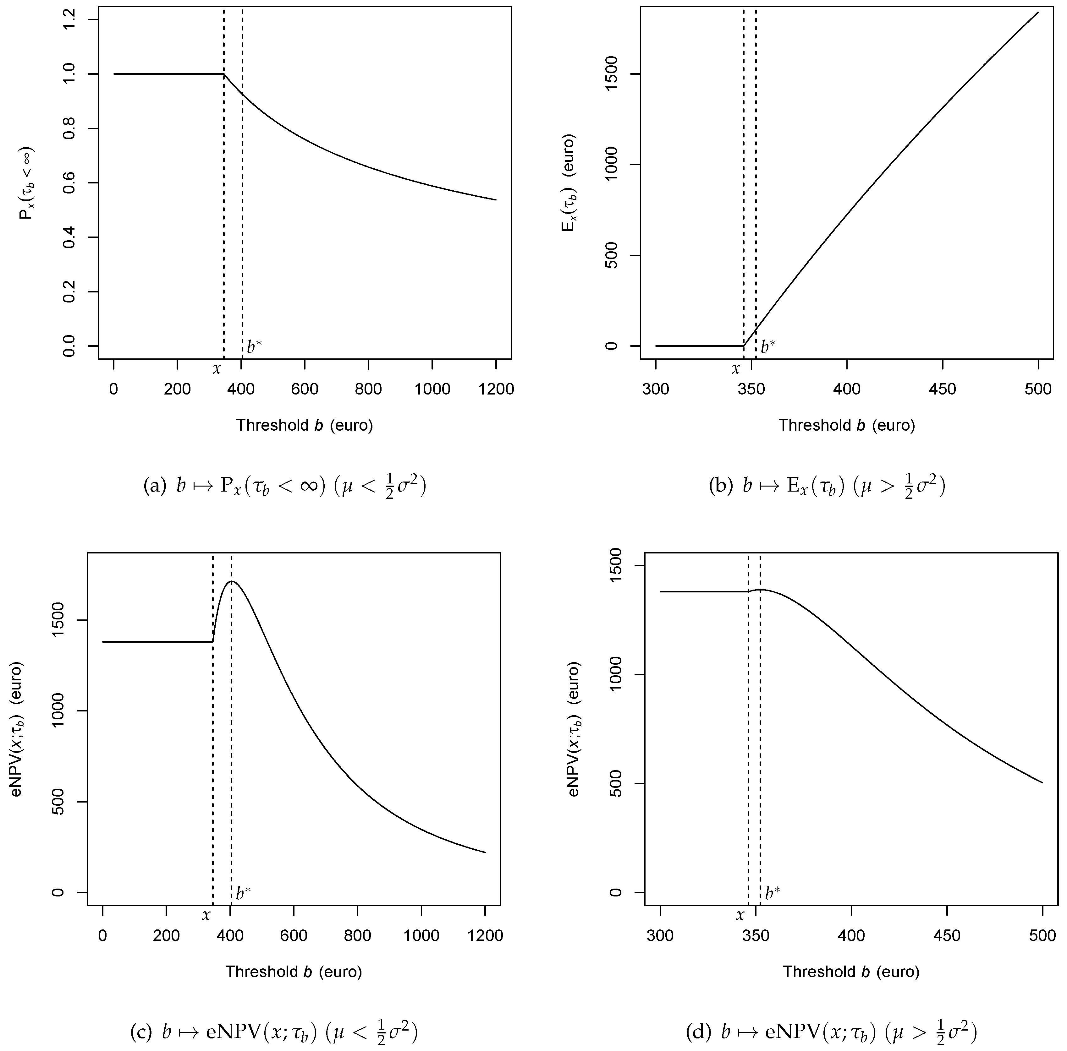
4.1. Distribution of the Hitting Time

In view of the formula (2), the hitting problem for the process $X_t$ is reduced to that for the Brownian motion with drift,

$${\tau }_b:=inf\{t\ge 0:X_t=b\}\equiv inf\{t\ge 0:B_t+\tilde{\mu }t=\tilde{b}\},$$

(58)

where

$$\tilde{\mu }=\frac{\mu -\frac{1}{2}{\sigma }^2}{\sigma },\tilde{b}=\frac{1}{\sigma }ln\frac{b}{x}.$$

(59)

Suppose that $x\le b$, so that $\tilde{b}\ge 0$. The explicit expression for the Laplace transform of the hitting time (58) is well known (see, e.g., Durrett 1999, Exercises 6.29 and 6.31, p. 268, or Etheridge 2002, Proposition 3.3.5, p. 61).

Proposition 1.

For $x\le b$ and any $\theta >0$, set

$${\mathsf{\Phi }}_{x,b}(\theta ):={\mathrm{E}}_x({\mathrm{e}}^{-\theta {\tau }_b})\equiv {\mathrm{E}}_x\left({\mathrm{e}}^{-\theta {\tau }_b}{\mathrm{𝟙}}_{\{{\tau }_b<\infty \}}\right).$$

(60)

Then

$${\mathsf{\Phi }}_{x,b}(\theta )=exp\left\{-\tilde{b}\left(\sqrt{\phantom{(}\tilde{\mu }{\phantom{\sigma }}^2+2\theta }-\tilde{\mu }\right)\right\},\theta >0,$$

(61)

where $\tilde{\mu }$ and $\tilde{b}$ are defined in (59).

Substituting the expressions (59), the formula (61) is rewritten as

$${\mathsf{\Phi }}_{x,b}(\theta )={\left(\frac{x}{b}\right)}^{q_1(\theta )},\theta >0,$$

(62)

where $q_1(\theta )$ is given by (cf. (24))

$$q_1(\theta )=\frac{1}{{\sigma }^2}\left(-(\mu -\frac{1}{2}{\sigma }^2)+\sqrt{{(\mu -\frac{1}{2}{\sigma }^2)}^2+2\theta {\sigma }^2}\right).$$

(63)

As usual, it is straightforward to extract from the Laplace transform (60) some explicit information about the distribution of the hitting time ${\tau }_b$. First, by the monotone convergence theorem (Shiryaev 1996, §II.6, Theorem 1(a), p. 186) we have

$$\underset{\theta \downarrow 0}{lim}{\mathsf{\Phi }}_{x,b}(\theta )={\mathrm{E}}_x({\mathrm{𝟙}}_{\{{\tau }_b<\infty \}})={\mathrm{P}}_x({\tau }_b<\infty ).$$

Hence, noting from (63) that

$$q_1(0)=\left\{\begin{array}{cc}0\hfill & \mathrm{if}\mu -\frac{1}{2}{\sigma }^2\ge 0,\hfill \\ 1-{\displaystyle \frac{2\mu }{{\sigma }^2}}\hfill & \mathrm{if}\mu -\frac{1}{2}{\sigma }^2<0,\hfill \end{array}\right.$$

(64)

we obtain

$${\mathrm{P}}_x({\tau }_b<\infty )={\left(\frac{x}{b}\right)}^{q_1(0)}=\left\{\begin{array}{cc}1,\hfill & \mu -\frac{1}{2}{\sigma }^2\ge 0,\hfill \\ {\left({\displaystyle \frac{x}{b}}\right)}^{1-2\mu /{\sigma }^2},\hfill & \mu -\frac{1}{2}{\sigma }^2<0.\hfill \end{array}\right.$$

(65)

Remark 5.

The result (65) shows that hitting the critical threshold $b=b^{*}$, as required by the stopping rule, is only certain when the wage growth rate is large enough, $\mu \ge \frac{1}{2}{\sigma }^2$. Thus, the “dangerous” case is when $\mu <\frac{1}{2}{\sigma }^2$, whereby relying only on the optimal stopping recipe may not be practical. This observation may serve as a germ of the idea to connect the optimality problem in the insurance context with the notion of utility (cf. the discussion in Section 7.1 below).

Via the Laplace transform ${\mathsf{\Phi }}_{x,b}(\theta )$, we can also obtain the mean hitting time ${\mathrm{E}}_x({\tau }_b)$ in the case $\mu \ge \frac{1}{2}{\sigma }^2$, where ${\tau }_b<\infty$ (${\mathrm{P}}_x$-a.s.). Namely, again using the monotone convergence theorem we have

$$\underset{\theta \downarrow 0}{lim}\frac{\partial {\mathsf{\Phi }}_{x,b}(\theta )}{\partial \theta }=-\underset{\theta \downarrow 0}{lim}{\mathrm{E}}_x({\tau }_b{\mathrm{e}}^{-\theta {\tau }_b})=-{\mathrm{E}}_x({\tau }_b).$$

Hence, differentiating formula (62) at $\theta =0$ and noting from (63) that $q_1(0)=0$ (cf. (64)) and

$$q_1^{\prime }(0)=\left\{\begin{array}{cc}\infty ,\hfill & \mu =\frac{1}{2}{\sigma }^2,\hfill \\ {\displaystyle \frac{1}{\mu -\frac{1}{2}{\sigma }^2}},\hfill & \mu >\frac{1}{2}{\sigma }^2,\hfill \end{array}\right.$$

we get

$${\mathrm{E}}_x({\tau }_b)=-ln\left(\frac{x}{b}\right){\left(\frac{x}{b}\right)}^{q_1(0)}{q}_1^{\prime }(0)=\left\{\begin{array}{cc}\infty ,\hfill & \mu =\frac{1}{2}{\sigma }^2,\hfill \\ {\displaystyle \frac{ln(b/x)}{\mu -\frac{1}{2}{\sigma }^2}},\hfill & \mu >\frac{1}{2}{\sigma }^2.\hfill \end{array}\right.$$

(66)

4.2. Alternative Derivation

An alternative (and more direct) method to derive the formulas (65) and (66) is based on general theory of Markov processes by solving the suitable boundary value problems (Øksendal 2003, §9). Namely, the hitting probability $\pi (x):={\mathrm{P}}_x({\tau }_b<\infty )$ as a function of $x>0$ satisfies the Dirichlet problem (Øksendal 2003, §9.2)

$$\left\{\begin{array}{c}\begin{array}{ccc}\hfill L\pi (x)& =0\hfill & \hfill (0<x<b),\\ \hfill \pi (b)& =1.\hfill & \end{array}\hfill \end{array}\right.$$

(67)

The differential equation in (67) reads

$$\frac{1}{2}{\sigma }^2{x}^2{\pi }^{″}(x)+\mu x{\pi }^{\prime }(x)=0(0<x<b),$$

which is easily solved to give

$$\pi (x)=c_1{x}^{1-2\mu /{\sigma }^2}+c_2.$$

If $1-2\mu /{\sigma }^2<0$ (i.e., $\mu -\frac{1}{2}{\sigma }^2>0$) then $c_1=0$ (since $\pi (x)$ is bounded), and due to the boundary condition $\pi (b)=1$ it follows that $c_2=1$ and $\pi (x)\equiv 1$. A similar argument shows that $\pi (x)\equiv 1$ in the case $1-2\mu /{\sigma }^2=0$. Finally, if $1-2\mu /{\sigma }^2>0$ then, noting that $\pi (0)=0$, we conclude that $c_2=0$ and, due to the boundary condition, $c_1=b^{-1+2\mu /{\sigma }^2}$. Thus, formula (65) is proved.

Similarly, the mean hitting time $m(x):={\mathrm{E}}_x({\tau }_b)$ (with $\mu -\frac{1}{2}{\sigma }^2>0$) satisfies the Poisson problem (Øksendal 2003, §9.3)

$$\left\{\begin{array}{c}\begin{array}{ccc}\hfill Lm(x)& =-1\hfill & \hfill (0<x<b),\\ \hfill m(b)& =0.\hfill & \end{array}\hfill \end{array}\right.$$

(68)

As usual, to solve the problem (68), it is convenient to approximate it with a two-sided boundary problem by adding an auxiliary Neumann (reflection) condition at $\epsilon >0$,

$$\left\{\begin{array}{c}\begin{array}{ccc}\hfill L{m}_{\epsilon }(x)& =-1\hfill & \hfill (\epsilon <x<b),\\ \hfill m_{\epsilon }(b)& =0,\hfill & \\ \hfill m_{\epsilon }^{\prime }(\epsilon )& =0,\hfill & \end{array}\hfill \end{array}\right.$$

(69)

and then taking the limit of $m_{\epsilon }(x)$ as $\epsilon \downarrow 0$. This procedure will produce the correct solution $m(x)$ since ${lim}_{\epsilon \downarrow 0}{\mathrm{P}}_x({\tau }_{\epsilon }<\infty )={\mathrm{P}}_x({\tau }_0<\infty )=0$ (for any $x>0$).

A particular solution to the inhomogeneous differential equation

$$\frac{1}{2}{\sigma }^2{x}^2{m}_{\epsilon }^{″}(x)+\mu x{m}_{\epsilon }^{\prime }(x)=-1(\epsilon <x<b)$$

can be sought in the form $m_0(x)=c_{0}lnx$, which gives $c_0=-1/(\mu -\frac{1}{2}{\sigma }^2)$. Thus, the general solution of (69) can be expressed as

$$m_{\epsilon }(x)=-\frac{lnx}{\mu -\frac{1}{2}{\sigma }^2}+c_1{x}^{1-2\mu /{\sigma }^2}+c_2.$$

(70)

Now, using the boundary conditions in (69) it is straightforward to check that

$$\underset{\epsilon \downarrow 0}{lim}{c}_1=0,\underset{\epsilon \downarrow 0}{lim}{c}_2=\frac{lnb}{\mu -\frac{1}{2}{\sigma }^2}.$$

Hence, from (70) we get

$$m(x)=\underset{\epsilon \downarrow 0}{lim}{m}_{\epsilon }(x)=\frac{ln\left(b/x\right)}{\mu -\frac{1}{2}{\sigma }^2},$$

which retrieves the result (66).

Remark 6.

The same method applied to the killed process ${\tilde{X}}_t$ with generator $\tilde{L}=L-\tilde{r}I$ (see (37)) provides a neat interpretation of the value function $u(x)$ as given by (43). Namely, rewrite the expectation in (33) (i.e., $\mathrm{e}\mathrm{NPV}(x;{\tau }_b)$) in the form ${\tilde{\mathrm{E}}}_x(g({\tilde{X}}_{{\tau }_b}))$, where ${\tilde{\mathrm{E}}}_x$ denotes expectation with respect to the killed process $({\tilde{X}}_t)$, and note that, for $b\ge 0$,

$${\tilde{\mathrm{E}}}_x\left(g({\tilde{X}}_{{\tau }_b})\right)=\left\{\begin{array}{cc}g(b){\tilde{\mathrm{P}}}_x({\tau }_b<\infty ),\hfill & x\in [0,b],\hfill \\ g(x),\hfill & x\in [b,\infty ).\hfill \end{array}\right.$$

In turn, the hitting probability $\tilde{\pi }(x):={\tilde{\mathrm{P}}}_x({\tau }_b<\infty )$ can be easily found by solving the corresponding Dirichlet problem (cf. (67)),

$$\left\{\begin{array}{c}\begin{array}{ccc}\hfill \tilde{L}\tilde{\pi }(x)& =0\hfill & \hfill (0<x<b),\\ \hfill \tilde{\pi }(b)& =1.\hfill & \end{array}\hfill \end{array}\right.$$

Indeed, repeating the calculations in Section 3.2, it is straightforward to get $\tilde{\pi }(x)={(x/b)}^{q^{*}}$.

4.3. Direct Maximization

Using the results of the previous sections, we can easily solve the optimal stopping problem (17), at least in the subclass of hitting times $\tau ={\tau }_b$ (see (33)),

$$u(x)=\underset{b\ge 0}{sup}\mathrm{e}\mathrm{NPV}(x;{\tau }_b)=\underset{b\ge 0}{sup}{\mathrm{E}}_x\left({\mathrm{e}}^{-\tilde{r}{\tau }_b}({\beta }_1{X}_{{\tau }_b}-P)\right).$$

(71)

Observe that if $x\ge b$ then ${\tau }_b=0$ and $X_{{\tau }_b}=x$ (${\mathrm{P}}_x$-a.s.), so that $\mathrm{e}\mathrm{NPV}(x;{\tau }_b)\equiv {\beta }_{1}x-P$ for all $b\in [0,x]$. Let now $b\in [x,\infty )$. As already noted, on the event $\{{\tau }_b<\infty \}$ we have $X_{{\tau }_b}=b$ (${\mathrm{P}}_x$-a.s.), hence, according to (17) and (62),

$$\mathrm{e}\mathrm{NPV}(x;{\tau }_b)=({\beta }_{1}b-P){\mathrm{E}}_x({\mathrm{e}}^{-\tilde{r}{\tau }_b})=({\beta }_{1}b-P){\left(\frac{x}{b}\right)}^{q_{*}}(b\ge x),$$

(72)

where $q_{*}=q_1{(\theta )|}_{\theta =\tilde{r}}$ (cf. (24) and (63)). It is straightforward to find the maximizer for the function (72). Indeed, the condition $(\partial /\partial b)\mathrm{e}\mathrm{NPV}(x;{\tau }_b)\ge 0$, equivalent to

$${\beta }_1{b}^{-q_{*}}-q_{*}({\beta }_{1}b-P)b^{-q_{*}-1}\ge 0,$$

holds for all $b\in [0,b^{*}]$, where

$$b^{*}=\frac{P{q}_{*}}{{\beta }_1(q_{*}-1)},$$

(73)

which is the same optimal threshold as before (cf. (23)). Thus, the supremum of $\mathrm{e}\mathrm{NPV}(x;{\tau }_b)$ over $b\ge x$ is attained at $b=b^{*}$ if $x\le b^{*}$ or at $b=x$ if $x\ge b^{*}$.

The corresponding value function $u(x)$ is then calculated as (cf. (25))

$$u(x)=\left\{\begin{array}{cc}{\displaystyle ({\beta }_1{b}^{*}-P){\left(\frac{x}{b^{*}}\right)}^{q_{*}},}\hfill & x\in [0,b^{*}],\hfill \\ {\displaystyle {\beta }_{1}x-P,}\hfill & x\in [b^{*},\infty ).\hfill \end{array}\right.$$

(74)

Finally, substituting (73) into (74), we obtain explicitly (cf. (26))

$$u(x)=\left\{\begin{array}{cc}{\displaystyle \frac{P}{q_{*}-1}{\left(\frac{{\beta }_1(q_{*}-1)x}{P{q}_{*}}\right)}^{q_{*}},}\hfill & {\displaystyle 0\le x\le \frac{P{q}_{*}}{{\beta }_1(q_{*}-1)},}\hfill \\ {\displaystyle {\beta }_{1}x-P,}\hfill & {\displaystyle \phantom{0\le }x\ge \frac{P{q}_{*}}{{\beta }_1(q_{*}-1)}.}\hfill \end{array}\right.$$

(75)

5. Statistical Issues and Numerical Illustration

5.1. Specifying the Model Parameters

From the practical point of view, in order to exercise the stopping rule (22), the individual concerned needs to be able to compute the critical threshold $b^{*}$ expressed in (23), for which the knowledge is required about ${\beta }_1$ (defined in (9)) and therefore about the parameters r, ${\lambda }_0$, $\mu$ and $\beta$ (see (5)); furthermore, to evaluate the quantity $q_{*}$ defined in (24), one needs to estimate $\mu -\frac{1}{2}{\sigma }^2$ and ${\sigma }^2$ itself. Specifically,

• The loss of job rate ${\lambda }_0$ can be extracted from the publicly available data about the mean length at work, which is theoretically given by $\mathrm{E}({\tau }_0)=1/{\lambda }_0$.
• Likewise, the inflation rate r is also in the public domain.
• To specify the wage growth rate $\mu$, a simple approach is just to set $\mu =r$ as a crude version of a “tracking” rule. However, it may be possible that the individual’s wage growth rate $\mu$ is, to some extent, stipulated by the job contract—for example, that it must not exceed the inflation rate r by more than 1% per annum (applicable, e.g., to civil servants) or, by contrast, that it must be no less than r minus 0.5% per annum (more realistic in the private sector). In practical terms, this would often mean that the actual growth rate $\mu$ is kept on the lowest predefined level.
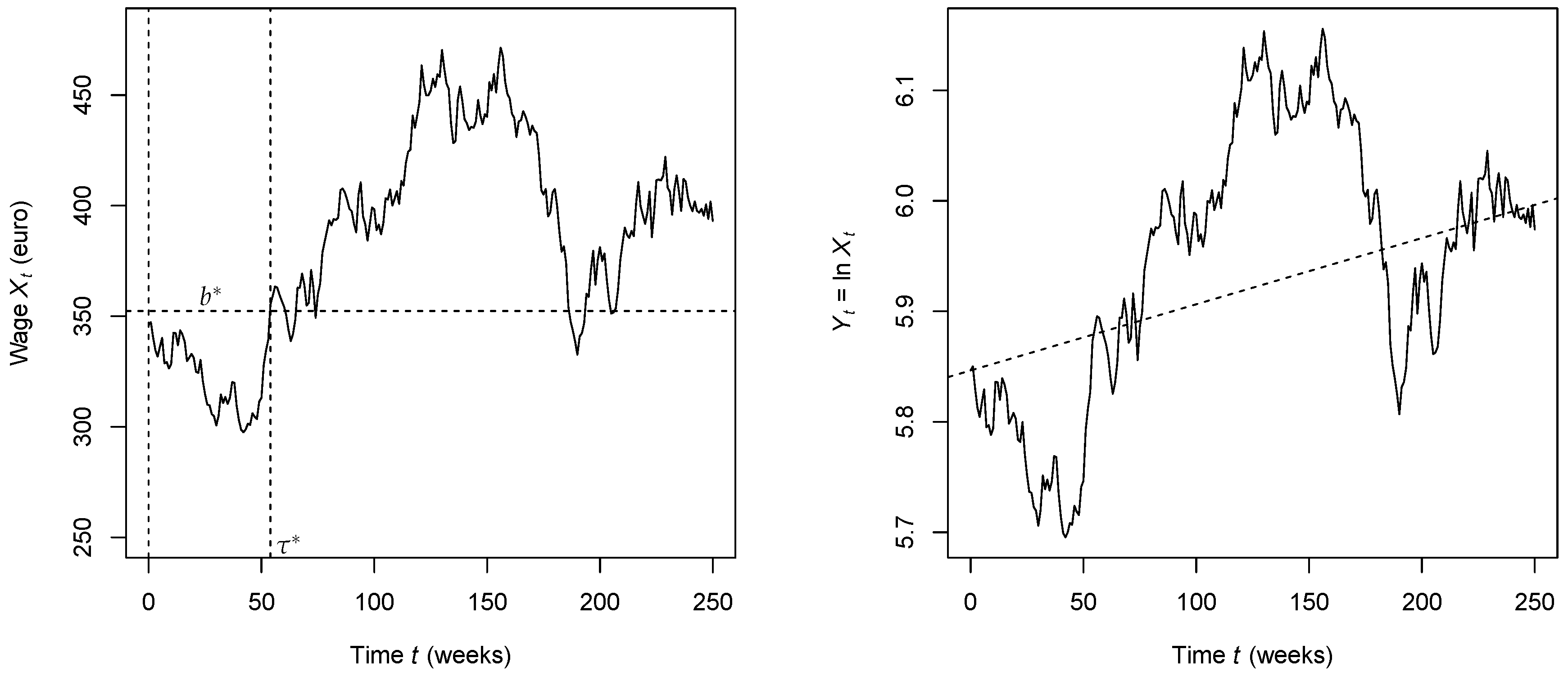
• More generally, the wage growth rate $\mu$ can be estimated by observing the wage process $X_t$. This can be implemented by first using regression analysis on $Y_t=ln{X}_t$ and estimating the regression line slope $\mu -\frac{1}{2}{\sigma }^2$ (see (2)). In addition, the volatility ${\sigma }^2$ can be estimated by using a suitable quadratic functional of the sample path $(Y_t)$.
• Finally, knowing the benefit schedule (which should be available through the insurance policy’s terms and conditions), it is in principle possible to calculate, or at least estimate the value $\beta$.

To summarize, certain estimation procedures need to be carried out along with the online observation of the sample path $(X_t)$. More details (most of which are quite standard) are provided in the next two subsections.

5.2. Estimating the Drift and Volatility

Denote for short $a:=\mu -\frac{1}{2}{\sigma }^2$. According to the geometric Brownian motion model (2), we have

$$Y_t:=ln{X}_t=lnx+\sigma B_t+at,Y_0=lnx.$$

Suppose the process $X_t$ is observed over the time interval $t\in [0,T]$ on a discrete-time grid $t_i=iT/n$ ($i=0,\cdots ,n$), and consider the consecutive increments

$$Z_i:=Y_{t_i}-Y_{t_{i-1}}=\sigma (B_{t_i}-B_{t_{i-1}})+a(t_i-t_{i-1})(i=1,\cdots ,n).$$

(76)

Note that the increments of the Brownian motion in (76) are mutually independent and have normal distribution with zero mean and variance $t_i-t_{i-1}=T/n$, respectively. Therefore, $(Z_i)$ is an independent random sample with normal marginal distributions,

$$Z_i\sim \mathcal{N}\left(\frac{aT}{n},\frac{{\sigma }^{2}T}{n}\right)(i=1,\cdots ,n).$$

Then, it is standard to estimate the parameters via the sample mean and sample variance,

$$\begin{array}{cc}\hfill {\widehat{a}}_n& :=\frac{n}{T}·\overline{Z}=\frac{Z_1+\cdots +Z_n}{T}=\frac{Y_T-Y_0}{T},\hfill \end{array}$$

(77)

$$\begin{array}{cc}\hfill {\widehat{\sigma }}_n^2& :=\frac{n}{T}·\frac{1}{n-1}\sum _{i=1}^n{(Z_i-\overline{Z})}^2.\hfill \end{array}$$

(78)

These estimators are unbiased,

$$\mathrm{E}({\widehat{a}}_n)=a=\mu -\frac{1}{2}{\sigma }^2,\mathrm{E}({\widehat{{\sigma }_n}}^2)={\sigma }^2,$$

with mean square errors

$$\mathrm{Var}({\widehat{a}}_n)=\frac{{\sigma }^2}{T},\mathrm{Var}({\widehat{\sigma }}_n^2)=\frac{2{\sigma }^4}{n-1}.$$

In turn, the parameter $\mu$ is estimated by

$${\widehat{\mu }}_n={\widehat{a}}_n+\frac{1}{2}{\widehat{\sigma }}_n^2,$$

with mean $\mathrm{E}({\widehat{\mu }}_n)=\mathrm{E}({\widehat{a}}_n)+\frac{1}{2}\mathrm{E}({\widehat{\sigma }}_n^2)=a+\frac{1}{2}{\sigma }^2=\mu$ and mean square error

$$\mathrm{Var}({\widehat{\mu }}_n)=\mathrm{Var}({\widehat{a}}_n)+\frac{1}{4}\mathrm{Var}({\widehat{\sigma }}_n^2)=\frac{{\sigma }^2}{T}+\frac{{\sigma }^4}{2(n-1)}$$

(due to independence of the estimators ${\widehat{a}}_n$ and ${\widehat{\sigma }}_n^2$).

Note that the estimator ${\widehat{a}}_n$ in (77) only employs the last observed value, $Y_T$; in particular, its mean square error is not sensitive to the grid size $\Delta t_i=T/n$, and only tends to zero with increasing observational horizon, $T\to \infty$. This makes the estimation of the drift parameter a difficult in the sense that very long observations over $Y_t$ are required to achieve an acceptable precision (Ekström and Lu 2011, Example 2.1, p. 3). For instance, let $\mu =0.004$ and $\sigma =0.02$ (per week), then $a=0.0038$; if $T=25$ (weeks) then the 95%-confidence bounds for a are given by $\widehat{a}\pm 1.96\sigma /\sqrt{T}=\widehat{a}\pm 0.00784$, so the margin of error is about twice as big as the value of a itself. To reduce it, say to $0.5a$, one needs $T\approx 425$ (weeks), which exemplifies slow convergence.

In contrast, the mean square error of the estimator ${\widehat{\sigma }}_n^2$ in (78) tends to zero as $n\to \infty$, with T fixed. Thus, estimation of the parameter ${\sigma }^2$ can be made asymptotically precise.

A numerical example illustrating the estimation of $\mu$ and ${\sigma }^2$ using simulated data will be given at the end of Section 5.4. A brief discussion of practical choices of $\mu$, based on sensitivity analysis, is provided at the end of Section 6.3.

5.3. Hypothesis Testing

In view of the drawback in the general solution of the optimal stopping problem in that the stopping time ${\tau }_{b^{*}}$ may be infinite, that is, ${\mathrm{P}}_x({\tau }_{b^{*}}=\infty )>0$, which occurs when $a=\mu -\frac{1}{2}{\sigma }^2<0$ (see Section 4.1), a reasonable pragmatic approach to decision-making in our model may be based on testing the null hypothesis $H_0:a\ge 0$ versus the alternative $H_1:a<0$ (at some intuitively acceptable significance level, e.g., $\alpha =0.05$). Namely, as long as $H_0$ remains tenable, one keeps waiting for the hitting time ${\tau }_{b^{*}}$ to occur, but once $H_0$ has been rejected, it is reasonable to terminate waiting and buy the policy immediately.

The corresponding test is specified as follows. Again, suppose that the process $Y_t$ is observed on a discrete time grid $t_i=iT/n$, and set $Z_i=Y_{t_i}-Y_{t_{i-1}}$ ($i=1,\cdots ,n$). Let $z(\alpha )$ be the upper $\alpha$-quantile of the standard normal distribution $\mathcal{N}(0,1)$, that is, $1-\mathsf{\Phi }(z(\alpha ))=\alpha$, where $\mathsf{\Phi }(x)=\frac{1}{\sqrt{2\pi }}{\int }_{-\infty }^x()-u^2/2\mathrm{d}u$. Then the null hypothesis $H_0:a\ge 0$ is to be rejected at significance level $\alpha$ whenever

$$Z_1+\cdots +Z_n\le \underset{a\ge 0}{inf}\left\{aT-z(\alpha )\sigma \sqrt{T}\right\},$$

that is,

$$Y_T-Y_0\le -z(\alpha )\sigma \sqrt{T}.$$

(79)

This test is uniformly most powerful among all tests with probability of error of type I not exceeding $\alpha$, that is, $\mathrm{P}(\mathrm{reject}{H}_0|H_0\mathrm{true})\le \alpha$.

The normal test (79) assumes that the variance ${\sigma }^2$ is known. As mentioned before, this presents no real restriction if the process $Y_t$ is observable continuously (i.e., if the grid $(t_i)$ can be refined indefinitely). If this is not the case (e.g., because the wage process can only be observed on the weekly basis) then the test (79) is replaced by the t-test,

$$Y_T-Y_0\le -t_{n-1}(\alpha )\widehat{\sigma }\sqrt{T},$$

where ${\widehat{\sigma }}^2$ is the sample variance (see (78)) and $t_{n-1}(\alpha )$ is the upper $\alpha$-quantile of the t-distribution with $n-1$ degrees of freedom.

In practice, the hypothesis testing is carried out sequentially (e.g., weekly) as the observational horizon T increases. The advantage of this approach is that the resulting stopping time is finite with probability one (i.e., ${\mathrm{P}}_x$-a.s.); indeed, it is the minimum between the optimal stopping time ${\tau }_{b^{*}}$ (which is finite ${\mathrm{P}}_x$-a.s. under the null hypothesis $H_0:a\ge 0$) and the first time of rejecting $H_0$ (which is finite ${\mathrm{P}}_x$-a.s. if $H_0$ is false).

5.4. Numerical Examples

To be specific, we use euro as the monetary unit. First of all, the value of the constant $\beta$, which encapsulates information about the benefit schedule as well as the rate ${\lambda }_1$ of finding new job (see (5)), is chosen to be

$$\beta =30.$$

Thus, the overall expected benefit payable over the lifetime of the policy (and projected to the beginning of unemployment) is taken to be equal to 30 weekly wages; that is, if the final wage is 400 (euro per week) then the total to be received is

$$400.00\times 30=12000.00(\mathrm{euro}).$$

Further, we set

$${\lambda }_0=0.01,r=0.0004.$$

This means that the expected time until loss of job is $1/{\lambda }_0=100$ (weeks), that is, about 1 year and 11 months, whereas the annual inflation rate is

$$()(365/7)·0.0004-1=0.02107617\approx 2.11\%,$$

which is quite realistic.

Next, we need to specify the premium P and the parameters of the wage process $X_t$, First, choose the initial value $x=X_0$ as

$$x=346.00(\mathrm{euro}).$$

This is motivated by the French labour legislation, whereby the current minimum pay rate is set as 9.88 euro per hour (WageIndicator 2018), with a 35-hour workweek (Estevão and Sá 2008; Gubian et al. 2004), giving

$$9.88\times 35=345.80(\mathrm{euro}\mathrm{per}\mathrm{week}).$$

As for the premium, it is set at the value

$$P=9000.00(\mathrm{euro}),$$

which equates to about 26 minimum weekly wages (i.e., income over about half a year). For simplicity, we also choose

$$\mu =r=0.0004,$$

(80)

so that the wage growth rate is the same as inflation r (in reality, it could be slightly less). Then from (9), using (80), we get

$${\beta }_1=\frac{{\lambda }_0\beta }{\tilde{r}-\mu }=\beta =30.$$

For the volatility $\sigma$, we will illustrate two opposite cases, $\mu <\frac{1}{2}{\sigma }^2$ and $\mu >\frac{1}{2}{\sigma }^2$.

Example 2.

Set $\sigma =0.04$, then $\mu -\frac{1}{2}{\sigma }^2=-0.0004<0$. From (24) we calculate $q_{*}=3.864208$, then (42) yields

$$b^{*}=404.7410=404.74(\mathrm{euro}).$$

Using (65), the hitting probability is calculated as

$${\mathrm{P}}_x({\tau }_{b^{*}}<\infty )=0.9245906.$$

Finally, using (43), we obtain the value of this contract,

$$v(346)=1714.2780=1714.28(\mathrm{euro}).$$

Example 3.

Now, set $\sigma =0.02$, then $\mu -\frac{1}{2}{\sigma }^2=0.0002>0$. Furthermore, using (24) we calculate $q_{*}=6.728416$, and from (42)

$$b^{*}=352.3705=352.37(\mathrm{euro}).$$

Hence, using (66), the expected hitting time is found to be

$$\mathrm{E}({\tau }_{b^{*}})=91.22197=91.2(\mathrm{weeks}).$$

Finally, according to formula (25), the value of this contract is calculated as

$$v(346)=1389.6190=1389.62(\mathrm{euro}).$$

In the simulation of the process $X_t$ shown in Figure 3, the drift $a=\mu -\frac{1}{2}{\sigma }^2$ is estimated using formula (77) as $\widehat{a}\doteq 0.0005994$. Estimation of the variance ${\sigma }^2$ according to formula (78) (on a weekly time grid) gives ${\widehat{\sigma }}^2\doteq 0.0003723$, while the true value is ${\sigma }^2=0.0004$. Hence, the parameter μ is estimated by $\widehat{\mu }\doteq 0.0007855$; recall that the true value is $\mu =0.0004$.

6. Parametric Dependencies

In this section, we aim to explore the parametric dependencies of the solution of our insurance problem, that is, of the optimal threshold $b^{*}$ given by (23) and the value function $v=v(x)$ given by (25). In particular, it is helpful to analyze different asymptotic regimes as well as (the sign of) appropriate partial derivatives, so as to ascertain the direction of changes under small perturbations and to understand their economic meaning. This is a key ingredient of sensitivity analysis and of the so-called comparative statics (Merton 1969, Section VII).

In what follows, we confine ourselves to a discussion of the two most important exogenous parameters—the wage drift $\mu$ and the unemployment rate ${\lambda }_0$. The constraint (11) implies that the range of the parameters $\mu$ and ${\lambda }_0$ is specified as follows,

$$-\infty <\mu <\tilde{r}=r+{\lambda }_0,0\vee (\mu -r)<{\lambda }_0<\infty .$$

Remark 7.

The next two technical subsections are elementary but rather tedious, and the reader wishing to grasp the results quickly may just inspect the plots in Figure 4 and Figure 5.

6.1. Monotonicity

By virtue of the quadratic Equation (40), the formula (23) can be conveniently rewritten as

$$b^{*}=\frac{P(\frac{1}{2}{\sigma }^2{q}_{*}+\tilde{r})}{\beta {\lambda }_0}.$$

(81)

First, fix ${\lambda }_0$ and consider the function $\mu \mapsto b^{*}$. Differentiating the Equation (23) and then again using (23) to eliminate $\mu$, we obtain

$$\frac{\partial q_{*}}{\partial \mu }=-\frac{q_{*}}{\frac{1}{2}{\sigma }^2(2q_{*}-1)+\mu }=-\frac{q_{*}^2}{\frac{1}{2}{\sigma }^2{q}_{*}^2+\tilde{r}}<0.$$

(82)

Hence, using (81) and (82),

$$\frac{\mathrm{d}{b}^{*}}{\mathrm{d}\mu }=\frac{\partial b^{*}}{\partial \mu }+\frac{\partial b^{*}}{\partial q_{*}}·\frac{\partial q_{*}}{\partial \mu }=-\frac{P(\frac{1}{2}{\sigma }^2{q}_{*}^2)}{\beta {\lambda }_0(\frac{1}{2}{\sigma }^2{q}_{*}^2+\tilde{r})}<0.$$

(83)

and, therefore, $b^{*}$ is a decreasing function of $\mu$ (see Figure 4a).

Similarly, the Equation (40) yields

$$\frac{\partial q_{*}}{\partial {\lambda }_0}=\frac{1}{\frac{1}{2}{\sigma }^2(2q_{*}-1)+\mu }=\frac{q_{*}}{\frac{1}{2}{\sigma }^2{q}_{*}^2+r+{\lambda }_0}>0.$$

(84)

From (81) and (84), after some rearrangements we obtain

$$\begin{array}{cc}\hfill \frac{\mathrm{d}{b}^{*}}{\mathrm{d}{\lambda }_0}& =\frac{\partial b^{*}}{\partial {\lambda }_0}+\frac{\partial b^{*}}{\partial q_{*}}·\frac{\partial q_{*}}{\partial {\lambda }_0}\hfill \\ \hfill & =-\frac{P(\frac{1}{2}{\sigma }^2{q}_{*}+r)}{\beta {\lambda }_0^2}+\frac{P(\frac{1}{2}{\sigma }^2{q}_{*})}{\beta {\lambda }_0(\frac{1}{2}{\sigma }^2{q}_{*}^2+r+{\lambda }_0)}\hfill \\ \hfill & =-\frac{P\left[(\frac{1}{2}{\sigma }^2{q}_{*}+r)(\frac{1}{2}{\sigma }^2{q}_{*}^2+r)+{\lambda }_{0}r\right]}{\beta {\lambda }_0^2(\frac{1}{2}{\sigma }^2{q}_{*}^2+r+{\lambda }_0)}<0,\hfill \end{array}$$

(85)

and it follows that the function ${\lambda }_0\mapsto b^{*}$ is decreasing (see Figure 4b).

Let us now turn to the value function $v=v(x)$. First, consider v as a function of $\mu$, thus keeping ${\lambda }_0$ fixed. Using the expression (23), we can rewrite the first line of the formula (25) (i.e., for $x\le b^{*}$) as

$$v=\frac{P}{q_{*}-1}{\left(\frac{x}{b^{*}}\right)}^{q_{*}}.$$

(86)

Differentiating (86), we get

$$\begin{array}{cc}\hfill \frac{\partial v}{\partial q_{*}}& =-\frac{P}{{(q_{*}-1)}^2}{\left(\frac{x}{b^{*}}\right)}^{q_{*}}\left(1+(q_{*}-1)ln\left(\frac{b^{*}}{x}\right)\right)<0,\hfill \end{array}$$

(87)

$$\begin{array}{cc}\hfill \frac{\partial v}{\partial b^{*}}& =-\frac{P{q}_{*}}{(q_{*}-1)b^{*}}{\left(\frac{x}{b^{*}}\right)}^{q_{*}}<0.\hfill \end{array}$$

(88)

Hence, on account of the inequalities (82), (84), (87) and (88),

$$\frac{\mathrm{d}v}{\mathrm{d}\mu }=\frac{\partial v}{\partial \mu }+\frac{\partial v}{\partial q_{*}}·\frac{\partial q_{*}}{\partial \mu }+\frac{\partial v}{\partial b^{*}}·\frac{\mathrm{d}{b}^{*}}{\mathrm{d}\mu }>0.$$

(89)

If $x\ge b^{*}$, then from the second line of (25) we readily obtain

$$\frac{\mathrm{d}v}{\mathrm{d}\mu }=\frac{\beta {\lambda }_{0}x}{{(\tilde{r}-\mu )}^2}>0.$$

(90)

Thus, in all cases $\mathrm{d}v/\mathrm{d}\mu >0$, which implies that the function $\mu \mapsto v$ is increasing (see Figure 5a).

Finally, fix $\mu$ and consider the function ${\lambda }_0\mapsto v$. If $x\ge b^{*}$, then v is given by the second line of (25), that is,

$$v=\frac{\beta {\lambda }_{0}x}{{\lambda }_0+r-\mu }-P.$$

(91)

In particular, if $\mu =r$, then (91) is reduced to $v\equiv v_{*}:=\beta x-P$. From (91) it follows that

$$\frac{\mathrm{d}v}{\mathrm{d}{\lambda }_0}=\frac{\beta x(r-\mu )}{{({\lambda }_0+r-\mu )}^2}\left\{\begin{array}{cc}\hfill <0,& \mu >r,\hfill \\ \hfill =0,& \mu =r,\hfill \\ \hfill >0,& \mu <r.\hfill \end{array}\right.$$

Due to monotonicity of the function ${\lambda }_0\mapsto b^{*}$ (see (85)), v is given by (91) as long as ${\lambda }_0\ge {\lambda }_{*}$, for some critical value ${\lambda }_{*}\equiv {\lambda }_{*}(\mu )\le \infty$. It will be shown below (see (99)) that ${lim}_{{\lambda }_0\to \infty }{b}_{*}=P/\beta$, so ${\lambda }_{*}<\infty$ if and only $x>P/\beta$. Clearly, ${\lambda }_{*}$ is determined by the condition $b^{*}=x$ (see (23)) together with the Equation (40). In the special case $\mu =r$ (assuming that $x>P/\beta$), these equations can be solved to yield

$${\lambda }_{*}=\frac{P}{\beta x}\left(\frac{\frac{1}{2}{\sigma }^2\beta x}{\beta x-P}+r\right).$$

(92)

In particular, in Example 3 this gives ${\lambda }_{*}\doteq 0.012420$. From the consideration above, it also follows that if $x>P/\beta$, then (see (91))

$$\underset{{\lambda }_0\to \infty }{lim}v=v_{*}=\beta x-P.$$

(93)

In the case $x\le b^{*}$, we use formula (86). Similarly to (89),

$$\frac{\mathrm{d}v}{\mathrm{d}{\lambda }_0}=\frac{\partial v}{\partial {\lambda }_0}+\frac{\partial v}{\partial q_{*}}·\frac{\partial q_{*}}{\partial {\lambda }_0}+\frac{\partial v}{\partial b^{*}}·\frac{\mathrm{d}{b}^{*}}{\mathrm{d}{\lambda }_0}.$$

(94)

Substituting the expressions (82), (84), (87), and (88) into (94), canceling immaterial factors and recalling formula (81), the condition $\mathrm{d}v/\mathrm{d}{\lambda }_0<0$ is reduced to

$$\left(\frac{1}{2}{\sigma }^2{q}_{*}+r\right)\left(\frac{1}{2}{\sigma }^2{q}_{*}^2+r\right)+{\lambda }_{0}r<\left(\frac{1}{q_{*}-1}+ln\left(\frac{b^{*}}{x}\right)\right)\left(\frac{1}{2}{\sigma }^2{q}_{*}^2+r+{\lambda }_0\right).$$

(95)

It can proved that if $\mu \ge r$, then the inequality (95) holds for all ${\lambda }_0<{\lambda }_{*}$, but the analysis becomes difficult for $\mu <r$. Numerical plots (see Figure 5b) suggest that in the latter case the function ${\lambda }_0\mapsto v$ may be non-monotonic, with the derivative $\mathrm{d}v/\mathrm{d}{\lambda }_0$ possibly vanishing in up to two points, provided that $r-\epsilon <\mu <r$ with $\epsilon >0$ small enough. To be more specific, the plots in Figure 5b illustrate the case $x>P/\beta$, with the common asymptote (93). For $x\le P/\beta$, the plots look similar (not shown here) but with ${lim}_{{\lambda }_0\to \infty }v=0$ (see (102) below), so the derivative $\mathrm{d}v/\mathrm{d}{\lambda }_0$ may vanish in at most one point.

6.2. Limiting Values

Let us investigate the functions $b^{*}$ and v in the limits (i) $\mu \to -\infty$ or $\mu \uparrow \tilde{r}$, and (ii) ${\lambda }_0\to \infty$ or ${\lambda }_0\downarrow 0$ ($\mu <r$), ${\lambda }_0\downarrow \mu -r$ ($\mu \ge r$). Start by observing, using Equation (40), that

$$\underset{\mu \to -\infty }{lim}{q}_{*}=\infty ,\underset{\mu \uparrow \tilde{r}}{lim}{q}_{*}=1,$$

(96)

and moreover,

$$q_{*}-1\sim \frac{\tilde{r}-\mu }{\frac{1}{2}{\sigma }^2+\tilde{r}}(\mu \uparrow \tilde{r}).$$

(97)

Similarly, ${lim}_{{\lambda }_0\to \infty }{q}_{*}=\infty$; on the other hand, if $\mu <r$ then ${lim}_{{\lambda }_0\downarrow 0}{q}_{*}=q_{*}{|}_{{\lambda }_0=0}>1$, while if $\mu \ge r$ then

$$q_{*}-1\sim \frac{{\lambda }_0-(\mu -r)}{\frac{1}{2}{\sigma }^2+\mu }({\lambda }_0\downarrow \mu -r).$$

(98)

Hence, from (81) and (96) it readily follows that $b^{*}\to \infty$ ($\mu \to -\infty$) and

$$b^{*}\to \frac{P(\frac{1}{2}{\sigma }^2+\tilde{r})}{\beta {\lambda }_0}(\mu \uparrow \tilde{r}).$$

Also, using that $q_{*}\to \infty$ (${\lambda }_0\to \infty$), from (23) we get

$$b^{*}\to \frac{P}{\beta }({\lambda }_0\to \infty ).$$

(99)

In the opposite limit, if $\mu >r$ then, according to (81) and (98),

$$b^{*}\to \frac{P(\frac{1}{2}{\sigma }^2+\mu )}{\beta (\mu -r)}({\lambda }_0\downarrow \mu -r),$$

(100)

while if $\mu \le r$ then ${lim}_{{\lambda }_0\downarrow 0}{b}^{*}=\infty$; in particular, for $\mu =r$

$$b^{*}\sim \frac{P(\frac{1}{2}{\sigma }^2+r)}{\beta {\lambda }_0}({\lambda }_0\downarrow 0).$$

(101)

For the value function $v=v(x)$, from formula (86) we get, using (96) and (97),

$$\underset{\mu \to -\infty }{lim}v=0,\underset{\mu \uparrow \tilde{r}}{lim}v=\infty .$$

Furthermore, according to (93), if $x>P/\beta$, then $v\to v_{*}=\beta x-P$ as ${\lambda }_0\to \infty$. In the opposite case, due to monotonicity of $b^{*}$ (see (85)) and the limit (99) we have $b^{*}>P/\beta \ge x$, so using formula (86) and recalling that $q_{*}\to \infty$, we get

$$v\le \frac{P}{q_{*}-1}\to 0({\lambda }_0\to \infty ).$$

(102)

Now, consider the limit of v as ${\lambda }_0$ approaches the lower edge of its range. If $\mu <r$ then (86) implies that ${lim}_{\lambda \downarrow 0}v=0$, since $b^{*}\to \infty$ and $q_{*}\to q_{*}{|}_{{\lambda }_0=0}>1$. If $\mu =r$ then, using (98) and (101) (with $\mu =r$), we obtain

$$v\sim \beta x{\lambda }_0^{q_{*}-1}=\beta xexp\left\{(q_{*}-1)ln{\lambda }_0\right\}\to \beta x({\lambda }_0\downarrow 0).$$

(103)

Finally, if $\mu >r$, then from (86) it readily follows, according to (98) and (100),

$$v\sim \frac{\beta x(\mu -r)}{\lambda -(\mu -r)}\to \infty ({\lambda }_0\downarrow \mu -r).$$

(104)

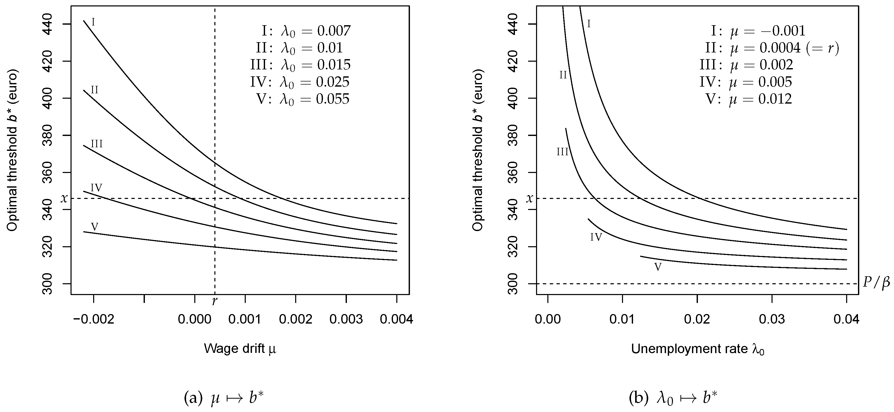
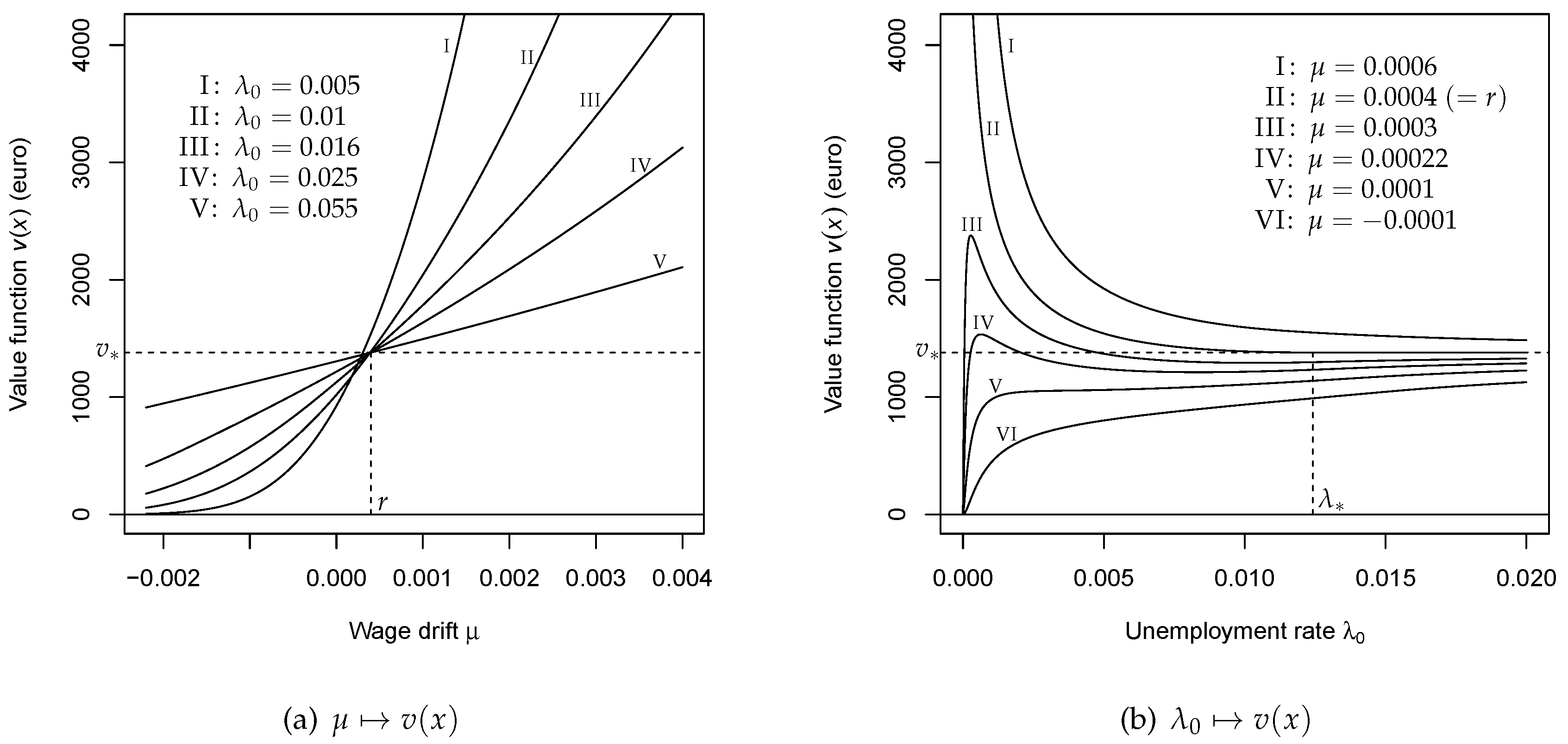
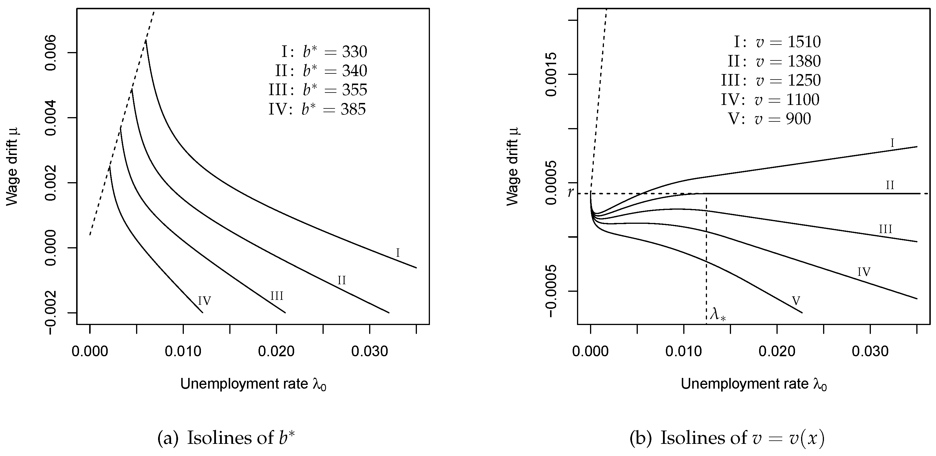
6.3. Comparative Statics and Sensitivity Analysis

The goal of comparative statics is to understand how varying values of exogenous parameters affect a target function of interest. For instance, consider the optimal threshold $b^{*}$ as a function of both unemployment rate ${\lambda }_0$ and wage drift $\mu$. Rather then fixing one of these parameters and then plotting $b^{*}$ against the remaining parameter (as was done in Figure 4), it is useful to plot a family of comparative statics plots showing the isolines (or level curves) for different values (levels) of the function, that is, $b^{*}({\lambda }_0,\mu )=\mathrm{const}$ (see Figure 6a). As may be expected from Figure 4, the plots of the function ${\lambda }_0={\lambda }_0(\mu )$ (determined implicitly by the level condition) behave as monotone decreasing graphs. Analogous plots for the value function are presented in Figure 6b; the plots become non-monotonic for v large enough. If ${\lambda }_0$ is fixed then the value v grows with $\mu$, in agreement with (89) and (90). Similarly, if $\mu >r$ is fixed then v decreases with ${\lambda }_0$, converging to the limit $v_{*}=\beta x-P$ as ${\lambda }_0\to \infty$ (see (93)), represented by curve II in Figure 5b. If $v>v_{*}$ then there are up to two different values of ${\lambda }_0$ (and common $\mu$) producing the same value v, while for v smaller than but close enough to $v_{*}$, the number of such roots may increase to three (see the discussion in Section 6.4).

Let us also comment on the sensitivity of our numerical examples presented in Section 5.4. The question here is, how much the output values (say, the optimal threshold $b^{*}$ and the value v) would change under a small variation of one of the background parameters. In the linear approximation, the change factor is given by the corresponding partial derivative. As in the previous sections, we address the sensitivity with regard to the wage drift $\mu$ (around the set value $\mu =0.0004$) and the unemployment rate ${\lambda }_0$ (around ${\lambda }_0=0.01$). Other model parameters are fixed as in Section 5.4, that is, $r=0.0004$, $P=9000$, $\beta =30$, and $x=346$. As for the volatility parameter $\sigma$, it is set to be $\sigma =0.04$ as in Example 2 or $\sigma =0.02$ as in Example 3. The required partial derivatives of $b^{*}$ and v can be computed using the formulas derived in Section 6.1; the results are presented in

Table 1. Sensitivity check of numerical results for the functions $b^{*}$ and v in Examples 2 and 3: (a) parametric derivatives and (b) increments in response to a $1\%$-change in the background parameters.

(a) Derivatives
Derivative	Example 2	Example 3
$\mathrm{d}{b}^{*}/\mathrm{d}\mu$	$-16037.57$	$-13962.43$
$\mathrm{d}v/\mathrm{d}\mu$	$842062.30$	$993991.20$
$\mathrm{d}{b}^{*}/\mathrm{d}{\lambda }_0$	$-6323.813$	$-3161.906$
$\mathrm{d}v/\mathrm{d}{\lambda }_0$	$-46485.530$	$-8768.435$
(b) Increments (euro)
Increment	Example 2	Example 3
$\Delta b^{*}$ ($\mu$)	$-0.06415$	$-0.05585$
$\Delta v$ ($\mu$)	$3.36825$	$3.97597$
$\Delta b^{*}$ (${\lambda }_0$)	$-0.63238$	$-0.31619$
$\Delta v$ (${\lambda }_0$)	$-4.64855$	$-0.87684$

a.

Numerical values in Table 1a may seem quite big, but they should be offset by small background values of the parameters, $\mu =0.0004$ and ${\lambda }_0=0.01$. If we increase them by a small amount, say by $1\%$, then the absolute increments would be

$$\Delta \mu =0.0004/100=4·{10}^{-6},\Delta {\lambda }_0=0.01/100={10}^{-4}.$$

Hence, using Table 1a, we obtain the corresponding approximate increments of the target functions $b^{*}$ and v (see Table 1b), which look more palatable. One interesting observation is that the value v reacts about 5 times stronger to the change of the unemployment rate ${\lambda }_0$ when the volatility $\sigma$ gets 2 times bigger (from $\sigma =0.02$ in Example 3 to $\sigma =0.04$ in Example 2); in contrast, the change of v in response to an increase of the wage drift is much less pronounced. This highlights the primary significance of the unemployment rate, which is of course only natural.

Sensitivity analysis with regard to the wage drift $\mu$ is also useful in the light of the difficulty in estimation of $\mu$ from the data, mentioned in Section 5.2. The results in Table 1b suggest that a reasonably small error in selecting $\mu$ has only a minor effect on the identification of the optimal threshold $b^{*}$ and the value v; for instance, overestimating it by $1\%$ will decrease $b^{*}$ by just $0.01$ euro, while the value v will be up by about $0.60$ euro. Thus, an individual using a moderately inflated value of their wage rate would take a slightly overoptimistic view about the timing of joining the insurance scheme and its expected benefit. On the other hand, a risk-averse individual may take a more conservative view and prefer to underestimate their wage drift $\mu$, which will raise the threshold $b^{*}$ resulting in a longer waiting time. For the insurance company though, it may be reasonable to try and avoid underestimation of the wage drift of potential customers, so as to reduce the risk of overpaying the benefits.

6.4. Economic Interpretation

Monotonic decay of the optimal threshold $b^{*}$ with an increase of the unemployment rate ${\lambda }_0$ (see (85) and Figure 4b) has a clear economic appeal: a bigger unemployment rate ${\lambda }_0$ means a higher risk of losing the job, which demands a lower target threshold $b^{*}$ in order to expedite joining the insurance scheme. The economic rationale for the monotonicity of $b^{*}$ as a function of $\mu$ (see (83) and Figure 4a) is different—a bigger wage drift $\mu$ makes it more likely to reach a higher final wage $X_{{\tau }_0}$ by the time of loss of job, so lowering the threshold $b^{*}$ adds incentive to an earlier entry.

Monotonic growth of the value v as a function of the wage drift $\mu$ (see (89), (90), and Figure 5a) is also meaningful—indeed, when the wage drift $\mu$ gets bigger, there is more potential to reach a higher final wage $X_{{\tau }_0}$ by the time of loss of job, which increases the expected benefit ${\beta }_1$ (see (9)) and, therefore, the value $v=v(x)$ of the insurance policy.

The behavior of the value function $v=v(x)$ in response to a varying unemployment rate ${\lambda }_0$ is more interesting, as indicated by the plots in Figure 5b. In the case $\mu <r$, it is satisfactory to see that the value v, vanishing in the limit as ${\lambda }_0\downarrow 0$, starts growing with ${\lambda }_0$, thus reflecting a good efficiency of the insurance policy against an increasing risk of unemployment. On the other side of the policy, this may present a growing risk for the insurance company which will have to finance an increasing number of claims. But with the unemployment rate ${\lambda }_0$ getting ever bigger, the value v should stay bounded, so must converge to a limit as ${\lambda }_0\to \infty$, given by $v_{*}=\beta x-P$ if $x>P/\beta$ (see (93)) or $v_{*}=0$ otherwise (see (102)). In particular, Figure 5b shows that, for a certain range of $\mu$, the value v achieves its maximum at some ${\lambda }_0$. However, the graphs also reveal that if $\mu$ keeps increasing then the value plots may have a more complicated non-monotonic behavior, which is harder to interpret economically.

On the other hand, as is evident from Figure 5b, in the case $\mu \ge r$ our model produces a counter-intuitive increase of the value v as ${\lambda }_0$ approaches the left edge of its range—it is hard to believe that the value may grow as the risk of unemployment falls. Moreover, as was computed in (104), for $\mu >r$ the corresponding limit of v is infinite! But perhaps the most striking example emerges in the borderline case $\mu =r$, whereby formally setting ${\lambda }_0=0$ we would get, according to (101), that the threshold $b^{*}$ is infinite (unlike the case $\mu >r$, see (101)), so that the wage process $(X_t)$ never reaches it; therefore, we never buy the insurance policy (understandably so, as there is no risk of losing the job), and nonetheless its value is positive in this limit (see (93)). The explanation of this paradox lies in the way how the optimal stopping is exercised for small ${\lambda }_0>0$: here, the threshold $b^{*}$ is high and there is only a very small probability that it is ever reached; before this happens, we stay idle, but if and when the threshold is hit then the expected payoff is rather big, which contributes enough to the expected net present value to keep it positive in the limit ${\lambda }_0\downarrow 0$ (see (103)).

Thus, the artefacts in our model as indicated above are caused by not putting any constraint on the waiting times. This can be rectified, for example, by introducing mortality, as was sketched in Section 2.3; in particular, such a regularization should restore a zero limit of v at the lower edge of ${\lambda }_0$.

7. Including Utility Considerations

7.1. Perpetual American Call Option

Our model (and its solution) resembles that of the optimal stopping problem for the (perpetual) American call option (see a detailed discussion in Shiryaev 1999, chp. VIII, §2a). More specifically, the holder of a call option may exercise the right to buy an asset (e.g., one unit of stock) at any time for a predetermined strike price K, where the decision is based on observations over the random process of stock prices $(S_t)$, assumed to follow a geometric Brownian motion model. The term perpetual is used to indicate that there is no expiration date, so the right to buy extends indefinitely.

The optimal time instant $\tau ={\tau }^{*}$ to buy, bearing in mind a purely financial target of maximizing the profit $S_{\tau }-K$, is the solution of the following optimal stopping problem,

$$V(x)=\underset{\tau }{sup}{\mathrm{E}}_x\left({\mathrm{e}}^{-r\tau }{(S_{\tau }-K)}^{+}\right),$$

(105)

where $S_t$ is a geometric Brownian motion with parameters $\mu <r$ and $\sigma >0$, the supremum is taken over all stopping times $\tau$ adapted to the filtration associated with $(S_t)$. The positive truncation ${(·)}^{+}$ corresponds to the constraint that the option holder is not in a position to buy at the price K higher than the current spot price $S_t$. The solution to (105) is well known (Shiryaev 1999, chp. VIII, §2a) to be given by the hitting time ${\tau }^{*}={\tau }_{b^{*}}$, with the optimal threshold

$$b^{*}=\frac{K{q}^{*}}{q^{*}-1},$$

where $q^{*}$ is given by formula (24) but with $\tilde{r}=r+{\lambda }_0$ replaced by r. The corresponding value function is given by

$$V(x)=\left\{\begin{array}{cc}(b^{*}-K){\left({\displaystyle \frac{x}{b^{*}}}\right)}^{q_{*}},\hfill & x\in [0,b^{*}],\hfill \\ x-K,\hfill & x\in [b^{*},\infty ).\hfill \end{array}\right.$$

Observe that our optimal stopping problem (17) can be rewritten as

$$v(x)={\beta }_1\underset{\tau }{sup}{\mathrm{E}}_x\left({\mathrm{e}}^{-\tilde{r}\tau }(X_{\tau }-\tilde{K})\right),\tilde{K}:=P/{\beta }_1,$$

(106)

which makes it look very similar to the perpetual American call option problem (105). However, there are several important differences. Firstly, unlike the gain function in the American call option problem (105), no truncation is applied in (106), because the financial gain is not the sole priority in this context and therefore the individual is prepared to tolerate negative values of ${\beta }_1{X}_{\tau }-P$ (despite the fact that, under the optimal strategy, the value function $v(x)$ is always non-negative, see Lemma 2(i) and formula (25)).5 In addition, as was mentioned in Remark 5 and in Section 5.3, the hitting time ${\tau }_{b^{*}}$ may be infinite with a positive probability (i.e., when $\mu <\frac{1}{2}{\sigma }^2$), which may be deemed impractical in the insurance context, but is considered to be acceptable for exercising the American call option. This simple observation helps to realize the fundamental conceptual difference between the two problems; indeed, the insurance optimal stopping does not focus only on the financial gain, but also places an ultimate priority on acquiring an insurance cover per se. Hence, a more realistic formulation of the optimal stopping problem in the UI model should involve a certain utility, which specifies the individual’s weighted preferences for satisfaction; for example, impatience against waiting for too long before joining the UI scheme.

7.2. Heuristic Optimal Stopping Models with Utility

Here, we present a few informal thoughts about the possible inclusion of utility in the optimality analysis. As already mentioned, in the case $\mu <\frac{1}{2}{\sigma }^2$ the probability of hitting the critical threshold $b^{*}$ is less than 1, so there is a probability that the individual will never join the insurance scheme if the optimal stopping rule is strictly followed. This is of course not desirable, as the individual puts high priority on getting insured at some point in time (hopefully, prior to loss of job).

One simple way to take these additional requirements into account is to extend the optimal stopping problem (17) as follows:

$$\begin{array}{cc}\hfill v^{†}(x)& =\underset{\tau }{sup}\left[\kappa {\mathrm{P}}_x(\tau <\infty )+\mathrm{e}\mathrm{NPV}(x;\tau )\right]\hfill \\ \hfill & =\underset{\tau }{sup}{\mathrm{E}}_x\left(\kappa {\mathrm{𝟙}}_{\{\tau <\infty \}}+{\mathrm{e}}^{-\tilde{r}\tau }g(X_{\tau })\right),\hfill \end{array}$$

(107)

where the supremum is again taken over all stopping times $\tau$ adapted to the process $(X_t)$, and the coefficient $\kappa \ge 0$ is a predefined weight representing the individual’s personal attitude (preference) towards the two contributing terms. If ${\mathrm{P}}_x(\tau <\infty )=1$ then the first term in (107) is reduced to a constant ($\kappa$), leading to a pure optimal stopping problem as before; however, if ${\mathrm{P}}_x(\tau <\infty )<1$ then the first term enhances the role of candidate stopping times $\tau$ that are less likely to be infinite.

The problem (107) can be rewritten in a more standard form by pulling out the common discounting factor under expectation,

$$v^{†}(x)=\underset{\tau }{sup}{\mathrm{E}}_x\left({\mathrm{e}}^{-\tilde{r}\tau }G(\tau ,X_{\tau })\right),$$

(108)

with

$$G(t,x):=\kappa {\mathrm{e}}^{\tilde{r}t}+g(x),(t,x)\in [0,\infty ]\times [0,\infty ).$$

(109)

Unfortunately, the optimal stopping problem (108) is not amenable to an exact solution as before, because the gain function (109) depends also on the time variable (Peskir and Shiryaev 2006, chp.IV). In this case, the problem (108) may again be reduced to a suitable (but more complex) free-boundary problem, but the hitting boundary (of a certain set on the $(t,x)$-plane) is no longer a straight line.

More generally, our optimal stopping problem can be modified by replacing the indicator in (107) with the expression ${\mathrm{e}}^{-\rho \tau }$ ($\rho >0$),

$$v^{†}(x)=\underset{\tau }{sup}{\mathrm{E}}_x\left(\kappa {\mathrm{e}}^{-\rho \tau }+{\mathrm{e}}^{-\tilde{r}\tau }g(X_{\tau })\right),$$

(110)

which retains the flavour of progressively penalizing larger values of $\tau$, including $\tau =\infty$. Here, the gain function (109) takes the form

$$G(t,x)=\kappa {\mathrm{e}}^{(\tilde{r}-\rho )t}+g(x).$$

In particular, by choosing $\rho =\tilde{r}$ the problem (110) is transformed into

$$v^{†}=\underset{\tau }{sup}{\mathrm{E}}_x\left({\mathrm{e}}^{-\tilde{r}\tau }({\beta }_1{X}_{\tau }+\kappa -P)\right),$$

which is the same problem as (17) but with the premium P replaced by $P-\kappa$.

Another, more drastic approach to amending the standard optimal stopping problem (17) stems from the observation that even if $\tau <\infty$ (${\mathrm{P}}_x$-a.s.), it may take long to wait for $\tau$ to happen—for instance, if ${\mathrm{E}}_x(\tau )=\infty$. In other words, it is reasonable to take into account the expected value of $\tau$, leading to the combined optimal stopping problem

$$v^{†}(x)=\underset{\tau }{sup}\left[\kappa {\mathrm{P}}_x(\tau <\infty )+\kappa exp\{-{\mathrm{E}}_x(\tau )\}+\mathrm{e}\mathrm{NPV}(x;\tau )\right].$$

(111)

If ${\mathrm{P}}_x(\tau <\infty )<1$ then ${\mathrm{E}}_x(\tau )=\infty$ and the problem (111) is reduced to (107), whereas if ${\mathrm{P}}_x(\tau <\infty )=1$ then, effectively, only the term with the expectation remains in (111). However, a disadvantage of the formulation (111) is that it cannot be expressed in the form (108). Trying to amend this would take us back to the version (110).

It is interesting to look at how the value function depends on the preference parameter $\kappa$. The next property is intuitively obvious.

Proposition 2.

For each $x>0$, the value function $v^{†}(x)$ of the optimal stopping problem (110) is a strictly increasing function of κ. The same is true for the problem (111).

Proof. 

We use the notation $v^{†}(x;\kappa )$ to indicate the dependence of the value function on the parameter $\kappa$. For ${\kappa }_1<{\kappa }_2$ and any stopping time $\tau \neg \equiv \infty$, we have

$${\mathrm{E}}_x\left({\kappa }_1{\mathrm{e}}^{-\rho \tau }+{\mathrm{e}}^{-\tilde{r}\tau }g(X_{\tau })\right)<{\mathrm{E}}_x\left({\kappa }_2{\mathrm{e}}^{-\rho \tau }+{\mathrm{e}}^{-\tilde{r}\tau }g(X_{\tau })\right)\le v^{†}(x;{\kappa }_2).$$

(112)

Suppose that ${\tau }_{*}$ is a maximizer for the optimal stopping problem (110) with $\kappa ={\kappa }_1$. Then, according to (112),

$$v^{†}(x;{\kappa }_1)={\mathrm{E}}_x\left({\kappa }_1{\mathrm{e}}^{-\rho {\tau }_{*}}+{\mathrm{e}}^{-\tilde{r}{\tau }_{*}}g(X_{{\tau }_{*}})\right)<v^{†}(x;{\kappa }_2),$$

that is, $v^{†}(x;{\kappa }_1)<v^{†}(x;{\kappa }_2)$ as claimed. Similar arguments apply to the problem (111). □

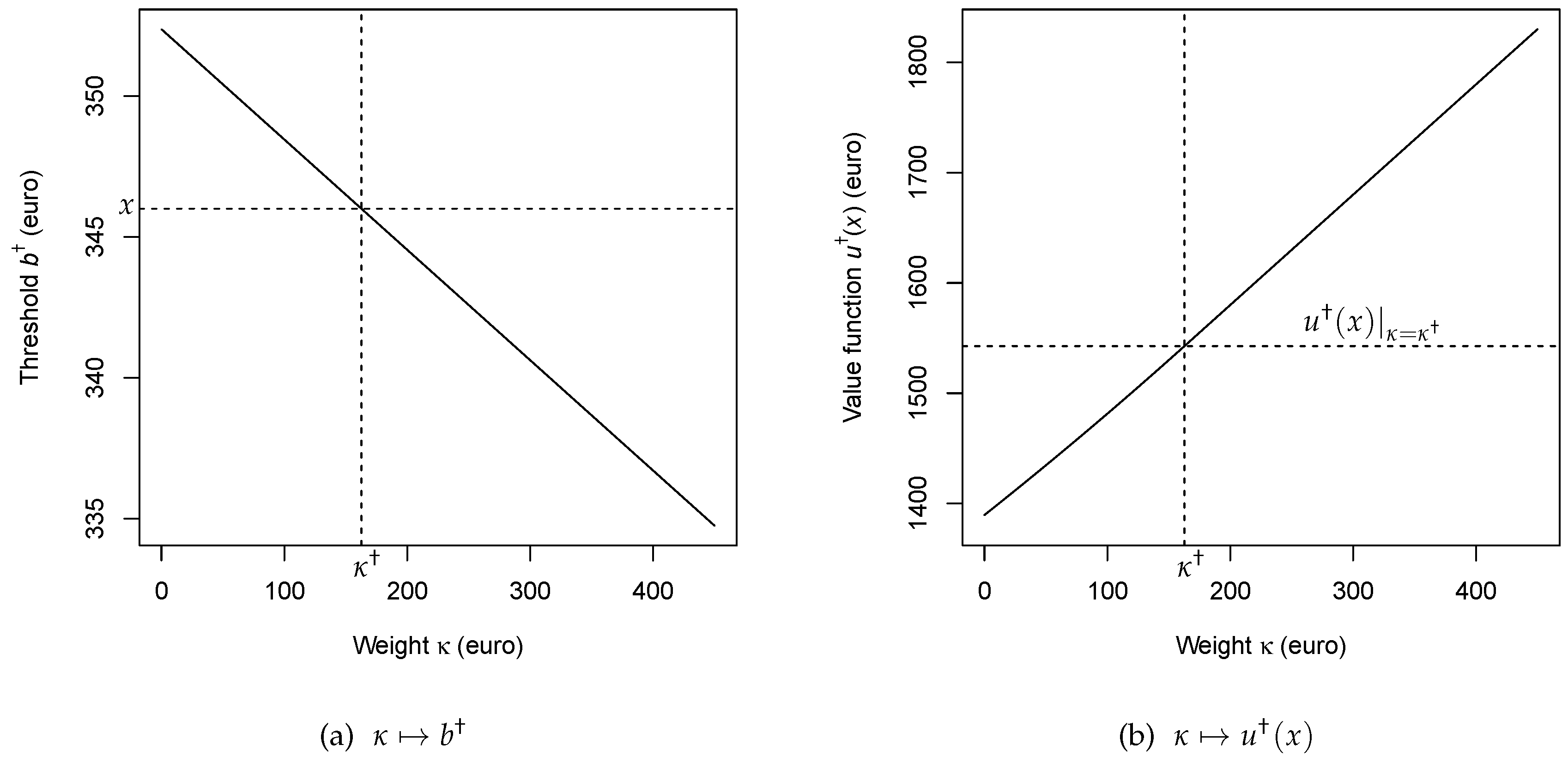
7.3. Suboptimal Solutions

As already mentioned, the optimal stopping problems outlined in Section 7.2 are difficult to solve in full generality. To gain some insight about the qualitative effects of the added utility-type terms, it may be reasonable to restrict our attention to solutions in the subclass of hitting times ${\tau }_b$. Despite such solutions will only be suboptimal, the advantage is that the reduced problems can be solved using that all the ingredients are available explicitly (see Section 4.1).

For example, the original problem (107) is replaced by

$$u^{†}(x)=\underset{b\ge 0}{sup}\left[\kappa {\mathrm{P}}_x({\tau }_b<\infty )+\mathrm{e}\mathrm{NPV}(x;{\tau }_b)\right].$$

(113)

Similarly as in Section 4.3, we only need to maximize the functional in (113) over $b\ge x$. Indeed, if $b\le x$ then ${\tau }_b=0$ (${\mathrm{P}}_x$-a.s.) and, according to (7) and (16),

$$\underset{b\le x}{sup}\left[\kappa {\mathrm{P}}_x({\tau }_b<\infty )+\mathrm{e}\mathrm{NPV}(x;{\tau }_b)\right]=\kappa +\mathrm{e}\mathrm{NPV}(x;0)=\kappa +{\beta }_{1}x-P,$$

whereas

$$\begin{array}{cc}\hfill \underset{b\ge x}{sup}\left[\kappa {\mathrm{P}}_x({\tau }_b<\infty )+\mathrm{e}\mathrm{NPV}(x;{\tau }_b)\right]& \ge {\left[\kappa {\mathrm{P}}_x({\tau }_b<\infty )+\mathrm{e}\mathrm{NPV}(x;{\tau }_b)\right]}_{b=x}\hfill \\ \hfill & =\kappa +{\beta }_{1}x-P.\hfill \end{array}$$

Assume that $\mu -\frac{1}{2}{\sigma }^2<0$ (for otherwise ${\mathrm{P}}_x({\tau }_b<\infty )=1$, thus leading to the same optimal stopping problem as before). Then, according to (65), the probability ${\mathrm{P}}_x({\tau }_b<\infty )$ becomes a strictly decreasing function of $b\in [x,\infty )$, and so the maximum in (113) is achieved by a different stopping strategy, with a lower optimal threshold $b^{†}$. More precisely, by virtue of formulas (65) and (72), the problem (113) is explicitly rewritten as

$$u^{†}(x)=\underset{b\ge x}{sup}\left[\kappa {\left({\displaystyle \frac{x}{b}}\right)}^{1-2\mu /{\sigma }^2}+({\beta }_{1}b-P){\left(\frac{x}{b}\right)}^{q_{*}}\right],$$

(114)

where $q_{*}>1$ is defined in (24). Differentiating with respect to b, it is easy to check that the maximizer for the problem (114) is given by

$$b^{†}=min\left\{b\ge x:a\kappa {\left(\frac{b}{x}\right)}^{q_{*}-a}+(q_{*}-1){\beta }_{1}b\ge P{q}_{*}\right\},$$

where $a:=1-2\mu /{\sigma }^2<1<q_{*}$.

The following (slightly artificial) version of the utility keeps the spirit of (113) but is amenable to the exact analysis:

$$u^{†}(x)=\underset{b\ge 0}{sup}\left[\kappa {\left\{{\mathrm{P}}_x({\tau }_b<\infty )\right\}}^{q_{*}/(1-2\mu /{\sigma }^2)}+\mathrm{e}\mathrm{NPV}(x;{\tau }_b)\right].$$

(115)

Indeed, using the same substitutions (65) and (72) as before, (115) is reduced to (cf. (114))

$$u^{†}(x)=\underset{b\ge x}{sup}\left[({\beta }_{1}b+\kappa -P){\left(\frac{x}{b}\right)}^{q_{*}}\right],$$

(116)

which is the same problem as (71) but with P replaced by $P-\kappa$ (cf. (72)). Therefore, from (73) we immediately obtain the maximizer

$$b^{†}=\frac{(P-\kappa )q_{*}}{{\beta }_1(q_{*}-1)}=b^{*}-\frac{\kappa q_{*}}{{\beta }_1(q_{*}-1)}\le b^{*}.$$

(117)

This is a strictly decreasing (linear) function of $\kappa$; in particular, $b^{†}=b^{*}$ if $\kappa =0$ and $b^{†}=0$ if $\kappa =P$. The corresponding value function is given by (cf. (74))

$$u^{†}(x)=\left\{\begin{array}{cc}{\displaystyle ({\beta }_1{b}^{†}+\kappa -P){\left(\frac{x}{b^{†}}\right)}^{q_{*}},}\hfill & x\in [0,b^{†}],\hfill \\ {\displaystyle {\beta }_{1}x+\kappa -P,}\hfill & x\in [b^{†},\infty ),\hfill \end{array}\right.$$

(118)

or more explicitly (cf. (75))

$$u^{†}(x)=\left\{\begin{array}{cc}{\displaystyle \frac{P-\kappa }{q_{*}-1}{\left(\frac{{\beta }_1(q_{*}-1)x}{(P-\kappa )q_{*}}\right)}^{q_{*}},}\hfill & {\displaystyle 0\le x\le \frac{(P-\kappa )q_{*}}{{\beta }_1(q_{*}-1)},}\hfill \\ {\displaystyle {\beta }_{1}x+\kappa -P,}\hfill & {\displaystyle \phantom{0\le }x\ge \frac{(P-\kappa )q_{*}}{{\beta }_1(q_{*}-1)}.}\hfill \end{array}\right.$$

(119)

If x is fixed then the problem value $u^{†}$, as a function of $\kappa$, is given by the first or the second line in (119) according as $\kappa \in [0,{\kappa }^{†}]$ or $\kappa \in [{\kappa }^{†},\infty )$, respectively, where

$${\kappa }^{†}:=P-\frac{{\beta }_1(q_{*}-1)x}{q_{*}}.$$

(120)

The dependence of $b^{†}$ and $u^{†}(x)$ upon the utility parameter $\kappa \in [0,P]$ is illustrated in Figure 7, while Figure 8 demonstrates the functional dependence of the hitting probability ${\mathrm{P}}_x({\tau }_b<\infty )$ and the mean hitting time ${\mathrm{E}}_x({\tau }_b)$ upon the variable threshold $b\ge 0$, along with the corresponding plots of the expected net present value $\mathrm{e}\mathrm{NPV}(x;{\tau }_b)$.

Remark 8.

Note that $u^{†}(x)$ is a strictly increasing function of $\kappa \in [0,P]$, in accord with Proposition 2. In particular, $u^{†}(x)$ coincides with the original value function $u(x)$ given by (75), but with the premium P replaced by $P-\kappa$. This can be interpreted as the individual’s consent to convert additional satisfaction, gained by virtue of pursuing the optimal stopping problem (115) instead of (17), into a higher premium, $P^{†}=P+\kappa$. Such an effect is characteristic of the use of risk-averse utility functions under the Expected Utility Theory (Kaas et al. 2008); see also a discussion below in Section 7.4.

In the case $\mu >\frac{1}{2}{\sigma }^2$, instead of (111) we may consider the simplified problem

$$u^{†}(x)=\underset{b\ge 0}{sup}\left[\kappa exp\{-{\mathrm{E}}_x({\tau }_b)\}+\mathrm{e}\mathrm{NPV}(x;{\tau }_b)\right].$$

(121)

Upon the substitution of formulas (66) and (72), it is rewritten in the form (cf. (114))

$$u^{†}(x)=\underset{b\ge x}{sup}\left[\kappa \frac{ln(b/x)}{\mu -\frac{1}{2}{\sigma }^2}+({\beta }_{1}b-P){\left(\frac{x}{b}\right)}^{q_{*}}\right].$$

(122)

Again, the maximization problem (122) can be solved (at least, numerically). For an analytic solution, it is convenient to modify the problem (121) as follows,

$$u^{†}(x)=\underset{b\ge 0}{sup}\left[\kappa exp\left(-\frac{q_{*}}{\mu -\frac{1}{2}{\sigma }^2}{\mathrm{E}}_x({\tau }_b)\right)+\mathrm{e}\mathrm{NPV}(x;{\tau }_b)\right].$$

Similarly to (122), this leads to the maximization problem that coincides with (116) and, therefore, has the same solution (117) and (118) (or, equivalently, (119)).

7.4. Connections to Expected Utility Theory

The considerations above can be linked to the standard Expected Utility Theory (Kaas et al. 2008). In the usual setting, it is assumed that an individual uses (perhaps, subconsciously) a certain utility $U(w)$, as a function of financial wealth w, to assess losses, gains and the resulting satisfaction. Generically, given the current wealth w and some random future loss Y, the expected loss (measured via utility $U(·)$) may be expressed as $\mathrm{E}\left[U(w-Y)\right]$. The individual is inclined to pay a premium P and buy the insurance policy as long as the expected utility without insurance is no more than $U(w-P)$,

$$\mathrm{E}[U(w-Y)]\le U(w-P).$$

(123)

The balance condition

$$\mathrm{E}[U(w-Y)]=U(w-P)$$

(124)

determines the maximum premium $P_{\max }$ the customer is prepared to pay (in fact, at this point it makes no difference whether to buy the insurance or not).

In the baseline case with $U(w)\equiv w$, the conditions (123) and (124) are reduced to

$$P\le P_{\max }=\mathrm{E}(Y).$$

(125)

However, choosing a different utility function may well change this threshold. For instance, if the random loss Y has exponential distribution with parameter $\theta =0.001$, then according to (125) we have $P_{\max }=\mathrm{E}(Y)=1/\theta =1000$. In contrast, let the utility function be chosen as $U(w)=1-exp\left(-\frac{1}{2}\theta w\right)$. Here, the utility is between 0 and 1 if the wealth w is positive, but it becomes increasingly negative for a negative wealth; that is, strong weight is placed against negative wealth, which may be characteristic of a risk-averse individual. In this case, it is easy to check that

$$P_{\max }=\frac{2ln2}{\theta }=1386.294>1000.$$

Thus, the individual is happy to pay more than before to protect themselves from the perceived risk of significant losses. That is to say, an additional amount of satisfaction is convertible into an extra premium.

In our case, if the UI was to be entered immediately, at time $t=0$, then the value of this decision would be $\mathrm{e}\mathrm{NPV}(x;0)={\beta }_{1}x-P$ (see (8) and (16)). Clearly, in order for this to be non-negative, the premium P must satisfy the condition

$$P\le P_{\max }={\beta }_{1}x.$$

For instance, in the setting of the numerical example in Section 5.4, we get $P_{\max }=30\times 346=10380$, while the set premium is $P=9000$.

Similarly, if the decision was taken at a stopping time $\tau$, then, conditional on the wage $X_{\tau }$, the maximum premium payable would be given by $P_{\max }={\beta }_1{X}_{\tau }$. Thus, the value of $P_{\max }$ goes up or down together with the current wage. However, in our setting the entry time is not decided in advance, being subject to the stopping rule based on observations over $(X_t)$. As a result, the value function $v(x)$ ($x>0$) of the optimal stopping problem is always positive for any premium P, no matter how high (see formula (26)). Apparently, this is manufactured by selecting the threshold $b^{*}$ high enough, which guarantees that, in the (rare) event of hitting it, the mean value of this strategy will be positive.

This may not be satisfactory from the standpoint of the Expected Utility Theory; however, there is no contradiction, because in its standard version this theory does not allow for an optional stopping. Adding utility terms to the gain function in the spirit of Section 7.2 and Section 7.3 helps to amend the situation (see Remark 8), but the maximum premium payable still remains indeterminate.

The explanation of this paradox lies in the simple fact that the gain function in the optimal stopping problems considered so far does not include any losses. A simple way to account for such losses is to include consumption in the model. Namely, suppose for simplicity that the consumption rate c is constant; for instance, the net present value of consumption over time interval $[0,t]$ is given by

$${\int }_0^t{\mathrm{e}}^{-rs}c\mathrm{d}s=\frac{c(1-{\mathrm{e}}^{-rt})}{r}.$$

It is natural to assume that the wage $X_t$ is sufficient to finance the consumption, so that ${\mathrm{E}}_x(X_t)=x{\mathrm{e}}^{\mu t}\ge c$ for all $t\ge 0$ (see (3)). In turn, for this to hold it suffices to assume that $X_0=x\ge c$ and $\mu \ge 0$. Hence, we need to take into account consumption only over the unemployment spell $[{\tau }_0,{\tau }_0+{\tau }_1]$, where the wage is replaced by the UI benefit. The expected net present value of this consumption is given by

$$\begin{array}{cc}\hfill \gamma :=\mathrm{E}\left(()-r{\tau }_0{\int }_0^{{\tau }_1}{\mathrm{e}}^{-rs}c\mathrm{d}s\right)& =\mathrm{E}({\mathrm{e}}^{-r{\tau }_0})·\mathrm{E}\left(\frac{c(1-{\mathrm{e}}^{-r{\tau }_1})}{r}\right)\hfill \\ \hfill & =\frac{{\lambda }_{0}c}{(r+{\lambda }_0)(r+{\lambda }_1)},\hfill \end{array}$$

using independence of ${\tau }_0$ and ${\tau }_1$ and their exponential distributions (with parameters ${\lambda }_0$ and ${\lambda }_1$, respectively). Thus, our basic optimal stopping problem (17) is modified to

$$v^{‡}(x)=\underset{\tau }{sup}{\mathrm{E}}_x\left([{\mathrm{e}}^{-\tilde{r}\tau }g(X_{\tau })-\gamma \right),$$

which has the same solution as before (see Section 2.5) but with the new value function $v^{‡}(x)=v(x)-\gamma$, that is (cf. (25)),

$$v^{‡}(x)=\left\{\begin{array}{cc}{\displaystyle ({\beta }_1{b}^{*}-P){\left(\frac{x}{{\displaystyle b^{*}}}\right)}^{q_{*}}-\gamma ,}\hfill & x\in [0,b^{*}],\hfill \\ {\displaystyle {\beta }_{1}x-P-\gamma ,}\hfill & x\in [b^{*},\infty ).\hfill \end{array}\right.$$

Now, the inequality $v^{‡}(x)\ge 0$ can be easily solved for P to yield

$$P\le P_{\max }^{‡}:=\left\{\begin{array}{cc}{\displaystyle {\beta }_1{b}^{*}-\gamma {\left(\frac{b^{*}}{x}\right)}^{q_{*}},}\hfill & x\in [0,b^{*}],\hfill \\ {\displaystyle {\beta }_{1}x-\gamma ,}\hfill & x\in [b^{*},\infty ).\hfill \end{array}\right.$$

(126)

Note that $P_{\max }^{‡}$ in (126) is a decreasing function of $\gamma$, but an increasing function of x. Thus, as could be expected, the maximum affordable premium gets lower with the increase of consumption, but becomes higher with the increase of the wage.

Remark 9.

Of course, consumption can also be incorporated into the optimal stopping models involving utility (see Section 6.3 and Section 7.2), but we omit technical details.

8. Concluding Remarks

In this paper, we have set up and solved an optimal stopping problem in a stylized UI model. The model and its solution are useful by illustrating approaches to optimal strategy of an individual seeking to get insured. By including consumption in the model, we have also demonstrated how a fair premium can be calculated, which makes our UI model usable also from the insurer’s perspective.

An explicit closed-form solution of the corresponding optimal stopping problem was possible due to some simplifying assumptions—in particular, exponential distribution of time ${\tau }_0$ to loss of job and constant inflation rate r. The analysis also strongly relied on the simplest model for the wage process $(X_t)$, that is, geometric Brownian motion with constant drift $\mu$ and volatility ${\sigma }^2$.

Let us indicate a few directions of making our UI model more realistic. Firstly, indefinite term of UI insurance could be replaced by a finite expiration term for the benefit schedule (akin to American call option with finite horizon), which would lead to a harder (time-dependent) optimal stopping problem (cf. Peskir and Shiryaev 2006, §25.2). Also, the assumption of exponential distribution of ${\tau }_0$ needs to be tested on the basis of real unemployment data. Note, however, that fitting a different distribution for ${\tau }_0$ will invalidate the expression (13) for the expected net present value $\mathrm{e}\mathrm{NPV}(x;\tau )$ and, therefore, will change the gain function in the optimal stopping problem (17), making it more difficult to solve.

The parameters of the model may also need to be made time-dependent, causing obvious complications to the model. On the other hand, the implicit assumption of passive waiting for a new job during the unemployment spell may not be realistic, or at least not desirable as individuals would rather be expected to seek jobs more proactively. Thus, it may be interesting to combine our UI model with job-seeking models such as in Boshuizen and Gouweleeuw (1995).

The inclusion of utility terms in the optimal setting is novel in this context, and illuminates significant changes in the individual’s behavior when driven by utility considerations. In particular, the value of the optimal stopping problem (110) is an increasing function of the preference coefficient $\kappa$ (see Proposition 2). This result is intuitively appealing, as it conforms with the usual impact of utility function (under the Expected Utility Theory), allowing one to convert extra satisfaction into extra premium. This is confirmed by our analysis of suboptimal solutions in Section 7.3 (see Figure 7). Finally, it would be interesting to study the optimal stopping problem (110) in more detail.

References

1. Acemoglu, Daron, and Robert Shimer. 2000. Productivity gains from unemployment insurance. European Economic Review 44: 1195–224. [Google Scholar] [CrossRef]
2. Baily, Martin Neil. 1978. Some aspects of optimal unemployment insurance. Journal of Public Economics 10: 379–402. [Google Scholar] [CrossRef] [Green Version]
3. Borch, Karl. 1961. The utility concept applied to the theory of insurance. ASTIN Bulletin 1: 245–55. [Google Scholar] [CrossRef]
4. Boshuizen, Frans A., and José M. Gouweleeuw. 1995. A continuous-time job search model: General renewal processes. Communications in Statistics. Stochastic Models 11: 349–69. [Google Scholar] [CrossRef]
5. Chen, Xiaoshan, Xun Li, and Fahuai Yi. 2019. Optimal stopping investment with non-smooth utility over an infinite time horizon. Journal of Industrial and Management Optimization 15: 81–96. [Google Scholar] [CrossRef] [Green Version]
6. Choi, Kyoung Jin, and Gyoocheol Shim. 2006. Disutility, optimal retirement, and portfolio selection. Mathematical Finance 16: 443–67. [Google Scholar] [CrossRef]
7. De Angelis, Tiziano, and Gabriele Stabile. 2019. On the free boundary of an annuity purchase. Finance and Stochastics 23: 97–137. [Google Scholar] [CrossRef]
8. Dhami, Sanjit. 2016. The Foundations of Behavioral Economic Analysis. Oxford: Oxford University Press. [Google Scholar]
9. Durrett, Rick. 1999. Essentials of Stochastic Processes, 1st ed. Springer Texts in Statistics. Springer: New York. [Google Scholar]
10. Ekström, Erik, and Bing Lu. 2011. Optimal selling of an asset under incomplete information. International Journal of Stochastic Analysis 2011: 543590. [Google Scholar] [CrossRef]
11. Estevão, Marcello, and Filipa Sá. 2008. The 35-hour workweek in France: Straightjacket or welfare improvement? (with comments by Barbara Petrongolo and panel discussion). Economic Policy 23: 417–63. [Google Scholar] [CrossRef]
12. Etheridge, Alison. 2002. A Course in Financial Calculus. Cambridge: Cambridge University Press. [Google Scholar] [CrossRef]
13. Fredriksson, Peter, and Bertil Holmlund. 2006. Optimal unemployment insurance design: Time limits, monitoring, or workfare? International Tax and Public Finance 13: 565–85. [Google Scholar] [CrossRef]
14. Gerrard, Russell, Bjarne Højgaard, and Elena Vigna. 2012. Choosing the optimal annuitization time post-retirement. Quantitative Finance 12: 1143–59. [Google Scholar] [CrossRef]
15. GoCompare. 2018. Unemployment Protection Insurance (Search & Comparison Web Site). Available online: www.gocompare.com/unemployment-protection (accessed on 22 August 2019).
16. Gubian, Alain, Stéphane Jugnot, Frédéric Lerais, and Vladimir Passeron. 2004. Les effets de la RTT sur l’emploi: Des estimations ex ante aux évaluations ex post (French). [The effects of the shorter working week on employment: From ex-ante simulations to ex-post evaluations.]. Économie et Statistique 376–377: 25–54. Available online: www.persee.fr/doc/estat_0336-1454_2004_num_376_1_7233 (accessed on 22 August 2019). [CrossRef]
17. Hairault, Jean-Olivier, François Langot, Sébastien Ménard, and Thepthida Sopraseuth. 2007. Optimal unemployment insurance in a life cycle model. Society for Economic Dynamics Meeting Papers, Paper 422. 25p. Available online: https://economicdynamics.org/meetpapers/2007/paper_422.pdf(accessed on 22 August 2019).
18. Henderson, Vicky, and David Hobson. 2008. An explicit solution for an optimal stopping/optimal control problem which models an asset sale. Annals of Applied Probability 18: 1681–705. [Google Scholar] [CrossRef]
19. Holmlund, Bertil. 1998. Unemployment insurance in theory and practice. Scandinavian Journal of Economics 100: 113–41. [Google Scholar] [CrossRef]
20. Hopenhayn, Hugo A., and Juan Pablo Nicolini. 1997. Optimal unemployment insurance. Journal of Political Economy 105: 412–38. [Google Scholar] [CrossRef]
21. Jang, Bong-Gyu, Seyoung Park, and Yuna Rhee. 2013. Optimal retirement with unemployment risks. Journal of Banking and Finance 37: 3585–604. [Google Scholar] [CrossRef]
22. Jensen, Uwe. 1997. An optimal stopping problem in risk theory. Scandinavian Actuarial Journal 1997: 149–59. [Google Scholar] [CrossRef]
23. Kaas, Rob, Marc Goovaerts, Jan Dhaene, and Michel Denuit. 2008. Modern Actuarial Risk Theory Using R, 2nd ed. Berlin: Springer. [Google Scholar] [CrossRef]
24. Karpowicz, Anna, and Krzysztof Szajowski. 2007. Double optimal stopping of a risk process. Stochastics 79: 155–67. [Google Scholar] [CrossRef]
25. Kerr, Kevin B. 1996. Unemployment compensation systems and reforms in selected OECD countries. Background Paper BP-415E, Library of Parliament, Parliamentary Research Branch. Ottawa: Government of Canada Publications, 22p. Available online: http://publications.gc.ca/collections/Collection-R/LoPBdP/BP-e/bp415-e.pdf(accessed on 22 August 2019).
26. Kolsrud, Jonas, Camille Landais, Peter Nilsson, and Johannes Spinnewijn. 2018. The optimal timing of unemployment benefits: Theory and evidence from Sweden. American Economic Review 108: 985–1033. [Google Scholar] [CrossRef]
27. Landais, Camille, Arash Nekoei, Peter Nilsson, David Seim, and Johannes Spinnewijn. 2017. Risk-based selection in unemployment insurance: Evidence and implications. IFS Working Paper W17/22. London: Institute for Fiscal Studies, 69p. [Google Scholar] [CrossRef]
28. Landais, Camille, and Johannes Spinnewijn. 2017. The value of unemployment insurance. CEPR Discussion Paper No. DP13624. London: Centre for Economic Policy Research (CEPR), 70p. Available online: https://cepr.org/active/publications/discussion_papers/dp.php?dpno=12364(accessed on 22 August 2019).
29. McCall, John J. 1970. Economics of information and job search. The Quarterly Journal of Economics 84: 113–26. [Google Scholar] [CrossRef]
30. Merton, Robert C. 1969. Lifetime portfolio selection under uncertainty: The continuous-time case. The Review of Economics and Statistics 51: 247–57. [Google Scholar] [CrossRef]
31. Merton, Robert C. 1971. Optimum consumption and portfolio rules in a continuous-time model. Journal of Economic Theory 3: 373–413. [Google Scholar] [CrossRef]
32. Muciek, Bogdan Krzysztof. 2002. Optimal stopping of a risk process: Model with interest rates. Journal of Applied Probability 39: 261–70. [Google Scholar] [CrossRef]
33. Neumann, John von, and Oskar Morgenstern. 1953. Theory of Games and Economic Behavior, 3rd ed. Princeton: Princeton University Press. [Google Scholar]
34. Øksendal, Bernt. 2003. Stochastic Differential Equations: An Introduction with Applications, 6th ed. Universitext. Berlin: Springer. [Google Scholar] [CrossRef]
35. Peskir, Goran, and Albert Shiryaev. 2006. Optimal Stopping and Free-Boundary Problems. Lectures in Mathematics, ETH Zürich. Basel: Birkhäuser. [Google Scholar] [CrossRef]
36. Pham, Huyên. 2009. Continuous-Time Stochastic Control and Optimization with Financial Applications. Stochastic Modelling and Applied Probability. Berlin: Springer, vol. 61. [Google Scholar] [CrossRef]
37. Rebollo-Sanz, Yolanda F., and J. Ignacio García-Pérez. 2015. Are unemployment benefits harmful to the stability of working careers? The case of Spain. SERIEs 6: 1–41. [Google Scholar] [CrossRef]
38. Shiryaev, Albert N. 1996. Probability, 2nd ed. Graduate Texts in Mathematics. New York: Springer, vol. 95. [Google Scholar] [CrossRef]
39. Shiryaev, Albert N. 1999. Essentials of Stochastic Finance: Facts, Models, Theory. Advanced Series on Statistical Science & Applied Probability; Singapore: World Scientific, vol. 3. [Google Scholar] [CrossRef]
40. Stabile, Gabriele. 2006. Optimal timing of the annuity purchase: Combined stochastic control and optimal stopping problem. International Journal of Theoretical and Applied Finance 9: 151–70. [Google Scholar] [CrossRef]
41. Villeneuve, Stéphane. 2007. On threshold strategies and the smooth-fit principle for optimal stopping problems. Journal of Applied Probability 44: 181–98. [Google Scholar] [CrossRef]
42. WageIndicator. 2018. Minimum Wages in France with effect from 01-01-2018 to 31-12-2018. Available online: https://wageindicator.org/salary/minimum-wage/france/archive/minimum-wages-in-france-with-effect-from-01-01-2018-to-31-12-2018 (accessed on 22 August 2019).
43. Wang, Tan, and Tony S. Wirjanto. 2016. Risk aversion, uncertainty, unemployment insurance benefit and duration of “wait” unemployment. Annals of Economics and Finance 7: 1–34. Available online: http://aeconf.com/Articles/May2016/aef170101.pdf (accessed on 22 August 2019).
44. Yeh, James. 1995. Martingales and Stochastic Analysis. Series on Multivariate Analysis; Singapore: World Scientific, vol. 1. [Google Scholar] [CrossRef]
1
For technical convenience, we choose to work with continuous-time models, but our ideas can also be adapted to discrete time (which may be somewhat more natural, since the wage process is observed by the individual on a weekly time scale).
2
Impact of individualistic (not always rational) perception in economics and financial markets is the subject of the modern behavioral economics (see, e.g., a recent monograph by Dhami 2016).
3
More specifically, according to the French UI system back in the 1990s (Kerr 1996, p. 8), a worker aged 50 or more, with eight months of insurable employment in the last twelve months, was entitled to full benefits equal to 57.4% of the final wage payable for the first eight months, thereafter declining by 15% every four months; however, the payments continued for no longer than 21 months overall. This leads to choosing the following numerical values in (6): h 0 = 0.574 , s 0 = 8 52 / 12 34.7 (weeks) and δ = ( 3 / 52 ) ln 1 0.15 0.0094 = 0.94 % (per week). The restriction of the benefit term by 21 52 / 12 = 91 weeks can be taken into account in our model by adjusting the parameter λ 1 from the condition E ( τ 1 ) = 91 , giving λ 1 0.0110 . A more conservative choice is to use a tail probability condition, for example, P ( τ 1 > 91 ) = 0.10 , yielding λ 1 = ln 0.10 / 91 0.0253 (with E ( τ 1 ) 39.5 ).
4
This conclusion is in accord with the general optimal stopping theory (Peskir and Shiryaev 2006, §2.2).
5
The equivalence of the problems (105) and (106), which we have established directly, is not a coincidence: it is known (Villeneuve 2007, Proposition 3.1, p.185) that, under mild assumptions, the solution of the general optimal stopping problem v ( x ) = sup τ E x e r τ g ( X τ ) does not change with the positive truncation of g ( · ) .
Figure 1. A time chart of the unemployment insurance scheme. The horizontal axis shows (continuous) time; the vertical axis indicates the pay rate (i.e., income receivable per unit time). The origin t = 0 indicates the start of employment. Two pieces of a random path X t depict the dynamics of the individual’s wage whilst in employment. The individual joins the UI scheme at entry time τ (by paying a premium P). When the current job ends (at time τ 0 > τ ), a benefit proportional to the final wage X τ 0 is payable according to a predefined schedule (e.g., see Example 1), until a new job is found after the unemployment spell of duration τ 1 .
Risks 07 00094 g001
Figure 2. Schematic diagram of possible transitions in the unemployment insurance scheme. Here, τ 0 and τ 1 are the (exponential) holding times in states 0 and 1, with parameters λ 0 and λ 1 , respectively, whereas τ is the entry time (i.e., from state 0– to state 0+), which is subject to optimal control based on observations over the wage process ( X t ) .
Risks 07 00094 g002
Figure 3. Simulated wage process X t (left) and Y t = ln X t (right) according to the geometric Brownian motion model (2), with X 0 = 346 (euros) and parameters μ = 0.0004 and σ = 0.02 (see Example 3). The dashed horizontal line in the left plot indicates the optimal threshold b * 352.37 (euros) first attained in this simulation at τ * = 54 (weeks). The dashed line in the right plot shows the estimated drift of the log-transformed data (see Section 5.2).
Risks 07 00094 g003
Figure 4. Graphs illustrating parametric dependencies of the optimal threshold (23): (a) on the wage drift μ < r ˜ and (b) on the unemployment rate λ 0 > 0 ( μ r ) , for selected values of λ 0 and μ , respectively. The values of other model parameters used throughout are as in Example 3: r = 0.0004 , P = 9 000 , β = 30 , and σ = 0.02 . The dashed horizontal line in both plots indicates the initial wage x = 346 . The dashed vertical line in (a) indicates μ = r . The lower dashed horizontal line in (b) shows the asymptote P / β = 300 (see (99)).
Risks 07 00094 g004
Figure 5. Graphs illustrating parametric dependencies of the value function (25): (a) on the wage drift μ < r ˜ and (b) on the unemployment rate λ 0 > 0 ( μ r ) , for selected values of λ 0 and μ , respectively. The values of other model parameters used throughout are as in Example 3: r = 0.0004 , P = 9000 , β = 30 , σ = 0.02 , and x = 346 . The dashed horizontal lines in both plots correspond to the value v * : = β x P = 1380 . The dashed vertical line in (a) indicates μ = r ; in this case, shown as curve II in plot (b), v ( x ) v * for all λ 0 λ * 0.012420 (see (92)). That is why curves III, IV and V in plot (a) all intersect at μ = r .
Risks 07 00094 g005
Figure 6. Isolines (level curves) of the optimal stopping problem solution on the ( λ 0 , μ ) -plane: (a) b * ( λ 0 , μ ) = const (optimal threshold (23)); (b) v ( λ 0 , μ ) = const (value function (25)). The values of other parameters used throughout are as in Example 3: r = 0.0004 , P = 9 000 , β = 30 , σ = 0.02 , and x = 346 . The slanted dashed lines in both plots show the boundary μ = λ 0 + r (see (11)). In plot b, the horizontal dashed line indicates μ = r and the vertical dashed line shows λ * 0.012420 (cf. Figure 5b).
Risks 07 00094 g006
Figure 7. Functional dependence on the preference weight κ in the reduced optimal stopping problem (115): (a) the optimal threshold b (see (117)) and (b) the value function u ( x ) (see (119)). Numerical values of the parameters used are as in Example 3: r = μ = 0.0004 , P = 9 000 , β = 30 , σ = 0.02 , and x = 346 . In particular, if κ = 0 then b coincides with b * 352.3705 and u ( x ) coincides with v ( x ) 1389.6190 . The dashed vertical lines on both plots indicate the value κ 162.7108 (see (120)) separating different regimes for u ( x ) according to (119). When κ = κ , we have b = x = 346 , shown as a dashed horizontal line in plot a; the corresponding value function is given by u ( x ) = β 1 x + κ P 1542.7110 (see (118)), shown as a dashed horizontal line in plot b. Note that the graph of u ( x ) in plot b looks almost linear for κ [ 0 , κ ] , because the ratio κ / P is quite small, 0 κ / P κ / P 0.01808 ; the slope here is approximately v ( x ) ( q * 1 ) / P 0.88448 , as compared to slope 1 of the linear graph for κ κ .
Risks 07 00094 g007
Figure 8. Theoretical graphs for functionals of the hitting time τ b versus threshold b 0 . Upper row: (a) the hitting probability P x ( τ b < ) (see (65)) and (b) the mean hitting time E x ( τ b ) (see (66)). Bottom row: the expected net present value e NPV ( x ; τ b ) (see (72)) with μ < 1 2 σ 2 (c) or μ > 1 2 σ 2 (d). The values of parameters used throughout are as in Section 5.4: x = 346 , P = 9 000 , β 1 = 30 , μ = 0.0004 , and σ = 0.04 (left) or σ = 0.02 (right). The dashed vertical lines in each plot indicate x and b * 404.7410 (left) (see Example 2) or b * 352.3705 (right) (see Example 3).
Risks 07 00094 g008