On the Validation of Claims with Excess Zeros in Liability Insurance: A Comparative Study

Abstract

In this study, we consider the problem of zero claims in a liability insurance portfolio and compare the predictability of three models. We use French motor third party liability (MTPL) insurance data, which has been used for a pricing game, and show that how the type of coverage and policyholders’ willingness to subscribe to insurance pricing, based on telematics data, affects their driving behaviour and hence their claims. Using our validation set, we then predict the number of zero claims. Our results show that although a zero-inflated Poisson (ZIP) model performs better than a Poisson regression, it can even be outperformed by logistic regression.

1. Introduction

There are two main types of machine learning: (i) predictive or supervised learning in which the machine trains data and learns the relationship between inputs and outputs and (ii) descriptive and unsupervised learning in which machine uses the inputs and discovers the outputs (Murphy 2012). Classification and regression are two supervised learning approaches which are well-known in general insurance. One of the objectives of the insurance companies is to charge premiums which is commensurate with the risk characteristics of their policyholders and for this, they classify the policyholders into homogeneous groups according to, say, age, sex, type of policy, subscription to telematics-based insurance pricing (see, Section 3), etc. Regression analysis and its extensions such as generalised linear modelling (GLM) are strong tools in insurance pricing. Unlike regression models, GLM is not constrained to a normal distribution and can be applied to any distribution from an exponential family. For example, a logistic regression model handles binary responses and thus is suitable for a Bernoulli distribution and a Poisson regression model applies to count data and deals with discrete random variables. GLM has long been used in actuarial practice to model claims amounts and claims frequency in the insurance portfolio (Haberman and Renshaw 1996; McCullagh and Nelder 1998).

In this study, we consider motor third party liability (MTPL) insurance. One of the problems in modelling claims frequency in this class of insurance is the number of zero claims and building a model that can capture all these zero claims. Zero claims in MTPL does not necessarily mean that there has been no accident during the term of a policy, rather it means that there has been no reported accident to the insurance company. This particularly happens under a no claim discount (NCD) system as some policyholders, known as bonus hunger, prefer to benefit from a discount by not reporting a claim. Another problem which is related to the previous one is the problem of over-dispersion. In a Poisson regression model, claims are distributed according to a Poisson distribution with equal mean and variance. Therefore, to build an appropriate model we need to test our dataset for the presence of over-dispersion (Peruman-Chaney et al. 2013; Wilson and Einbeck 2018). Binomial regression, negative binomial (NB) regression and zero-inflated Poisson (ZIP) model are techniques that can handle over and under dispersed data with the latter being able to distinguish between structured and unstructured zeros. Lambert (1992) considers a ZIP model where the probability of only possible observation, i.e., 0 and the parameter of a Poisson distribution depend on some covariates. Lambert (1992) applies this technique to model the number of defects in manufacturing. Since then, this model has been applied in different settings including insurance pricing. For example, Lee et al. (2002) use this model to analyse the impact of lifestyle and motivations on car crashes involving young drivers in Australia. Yip and Yau (2005) use ZIP to model claims frequency in car insurance. They compare different types of zero-inflated count models and conclude that a zero-inflated double Poisson regression model is a good fit for their dataset. Boucher et al. (2007) compare zero-inflated, hurdle and compound frequency models and conclude that the bonus rate is an important factor for policyholders to report the claim. In another study, Boucher et al. (2009) consider the problem of bonus hunger and construct a ZIP model to distinguish between the distribution of the number of claims and the number of accidents.

Model fitting and the selection of risk factors can be challenging in some cases. There are some papers that consider these problems. For example, Tang et al. (2014) propose a method to determine the variables in a ZIP model. They combine EM algorithm and adaptive LASSO and find that their technique performs better for the non-inflated part of the ZIP regression. Liu and Pitt (2017) also apply LASSO and ridge regression to address this issue in a bivariate negative binomial regression model. See, also, Cantoni and Auda (2018), Chowdhury et al. (2019) and Chen et al. (2019) among others.

The impact of mileage as a risk factor is considered by Lemaire et al. (2015). They conclude that annual mileage is a powerful predictor of the number of claims at-fault. Tselentis et al. (2017) provide a review of some Usage-based motor insurance (UBI) including Pay-as-you-drive (PAYD), Pay-how-you-drive (PHYD) and Pay-at-the-pump (PATP). PATP is a pricing method that considers fuel consumption as a rating factor but did not get enough attention from researchers. These new pricing methods require telematics data. In recent years, there is much research on telematics data and mileage based (MB) insurance. Boucher et al. (2017) apply generalised additive models and consider both time and mileage in insurance pricing. See the following papers on the relevance of including the mileage as a risk factor (Ayuso et al. 2019; Guillen et al. 2019; Verbelen et al. 2018).

In addition to regression analysis, neural network, decision tree, random forest and boosting algorithms such as XGBoost, etc., are other machine learning techniques that can be applied to model claims frequency and insurance pricing. However, although these models have good predictive power, unlike regression models, it is difficult to interpret their parameters and their computation time is long. Weerasinghe and Wijegunasekara (2016) study neural network, decision tree and multinomial logistic regression models. Their results show that the neural network has the best predictive performance among the three models. However, they state that to understand the relationship between independent and dependent variables, the logistic regression is the best model. Fauzan and Murfi (2018) compare XGBoost, neural network and random forest models and find that in terms of the Gini index, XGBoost is a more accurate algorithm. See, also, Spedicato et al. (2018) and Gao et al. (2019) and the references therein.

In this study, we consider the classical Poisson and logistic regression and compare our findings with a ZIP model. We divide our dataset into training and validation (hold-out) set to predict the number of zero claims. This paper is organised as follows. In the next section, we present models and notation. Section 3 discusses our dataset. In Section 4, we build our models and in Section 5 we test their validation. Finally, Section 6 concludes.

2. Methodology and Notation

Risk classification is an important concept in general insurance pricing. An insurance company tries to determine the insurance premium according to risk characteristics of policyholders such as age, sex, type of policy and car model, etc. Regression analysis is a well-known technique to incorporate such risk (rating) factors. In this section, we review Poisson regression, Logistic regression and ZIP model.

Let $y_i\in \{0,1,2,\cdots \}$ be a dependent or response variable such as number of claims, for $i=1,\cdots ,n$ that follows a Poisson distribution with parameter ${\lambda }_i$. Assuming a log link function and that ${\lambda }_i$ is a linear combination of rating factors ${\beta }_0+{\beta }_1{x}_{i1}+\cdots +{\beta }_k{x}_{ik}$ we have

$$\begin{array}{c}\hfill E\left[y_i\right|x_i]={\lambda }_i=exp\{{\beta }_0+{\beta }_1{x}_{i1}+\cdots +{\beta }_k{x}_{ik}\},y_i\sim \mathrm{Pois}\left({\lambda }_i\right)\mathrm{for}i=1,2,\cdots ,n.\end{array}$$

(1)

When we consider the average number of claims for each policyholder, we need to specify a unit measure or exposure. We cannot expect two policyholders with the same risk characteristics, but different terms, to be equally risky. Normally, the length of coverage is considered as an exposure. However, in recent years, it is argued that even if policyholders join at different times, some may drive fewer distances than others. Therefore, when such information is available as in telematics data, mileage travelled is considered as a more appropriate exposure (Guillen et al. 2019). In our study, all policyholders are under observation for one year and thus the exposure for each policyholder is 1.

We use logistic regression when $y_i\in \{0,1\}$ is a binary, also called dichotomous variable. In that case,

$$\begin{array}{c}\hfill E\left[y_i\right|x_i]={\pi }_i\left(x\right)=g\left({\beta }_0+{\beta }_1{x}_{i1}+\cdots +{\beta }_k{x}_{ik}\right)\end{array}$$

where g is a logistic link function to ensure that ${\pi }_i$ is between 0 and 1. Hence

$$\begin{array}{c}\hfill {\pi }_i\left(x\right)=\frac{exp\left\{{\beta }_0+{\beta }_1{x}_{i1}+\cdots +{\beta }_k{x}_{ik}\right\}}{1+exp\left\{{\beta }_0+{\beta }_1{x}_{i1}+\cdots +{\beta }_k{x}_{ik}\right\}}\end{array}$$

(2)

or, more commonly

$$\begin{array}{c}\hfill log\left(\frac{{\pi }_i\left(x\right)}{1-{\pi }_i\left(x\right)}\right)={\beta }_0+{\beta }_1{x}_{i1}+\cdots +{\beta }_k{x}_{ik}.\end{array}$$

In this paper, we use logistic regression to answer the question: “What is the probability of a claim $(y_i=1)$ and zero claims $(y_i=0)$ for a given policyholder with particular risk characteristics?”

When the mean and variance of the underlying population is not equal, the assumption of a Poisson distribution is not suitable and a better candidate is a distribution that can allow for over/under dispersion such as a binomial or NB distribution. However, sometimes we deal with a large number of zeros in our dataset. For example, we see in the next section that many policyholders have zero claims, which does not necessarily mean that they were involved in no accidents, but they are low risk. In such cases, we can apply a ZIP model which is a mixture of a point mass at zero, also called structural zeros, and another claims frequency distribution, such as a Poisson or NB, which can be written as

$$\begin{array}{c}\hfill \mathrm{Pr}(y_i=j)=\left\{\begin{array}{cc}{\pi }_i+(1-{\pi }_i)\mathrm{Pr}(y_i=0)\hfill & j=0\hfill \\ (1-{\pi }_i)\mathrm{Pr}(y_i=j)\hfill & j=1,2,\cdots \hfill \end{array}\right.\end{array}$$

(3)

where ${\pi }_i$ is given by Equation (2) and denotes the probability of zeros when zero is the only possible observation. In a ZIP model, $y_i$ follows a Poisson distribution with parameters being given by Equation (1).

We can easily implement these models in R and the codes are provided in Appendix A (Frees et al. 2014, 2016).

3. Data

We use datasets provided by the French Institute of Actuaries for the 2017 pricing game, which is based on French MTPL insurance. The dataset is available in Package ‘CASdatasets’ by Dutang and Dutang and Charpentier (2019) and to the best of the author’s knowledge, this is the first time it is used in a study. The dataset contains some information about the new pricing strategy of the company. The policyholders were given a choice whether they would like to join a new mileage-based (MB) pricing system or not. We would like to see how policyholders’ perception regarding this new system affects their driving behaviour and hence their number of claims. There are two types of datasets: (i) underwriting and (ii) claims dataset. Underwriting datasets are available for three years, whereas claims dataset is only publicly available for year 0. Therefore, we only use data from year 0. After merging claims and underwriting datasets, we randomly split our data into training and validation sets with $60\%$ being in training and $40\%$ in the validation set. As some policyholders have more than one car, we assume that each policy covers only one car and therefore consider the number of policies and claims per policy rather than claims per policyholder. We have 100,000 policies (rows in underwriting dataset) and 12,654 policies with claims (rows in claims dataset after consolidation).

Table 1. Variables in our datasets.

Control	Policy	Driver (1 and 2)	Vehicle	Response
policy ID	bonus coefficient	driver 2?	age	number of claims
	type of coverage	age	cylinder
	duration	gender	din power
	situation duration		fuel type
	payment frequency		max speed
	subscription to MB		type
	usage		value
			weight

shows the variables we use in our study. In addition to these variables, information about Insee town code, make and model, marketing duration and age of driving license are also provided. However, we do not take into account these variables as, for example, there is a considerable number of policies with 113 years for driving license age which is not reasonable.

In Table 1 policy ID refers to the combination of the vehicle ID and policyholder ID. In this study, we have 100,000 policy ID. Bonus coefficient is the percentage of the full premium that policyholders pay allowing for their claims experience and the allocated discount. There are four types of coverage available: Maxi, Median 2, Median 1 and Mini. The time from the last policy alteration, such as the inclusion of a new driver, is represented by situation duration. Payments can be made annually, semi-annually, quarterly and monthly. As it is usual for the liability insurance, some of the claims amounts are negative1. Therefore, we set all claims amounts of less than 30 equal to zero (Ferreira and Minikel 2012; Frees et al. 2014).

Subscription to mileage-based (MB) policy refers to a new scheme in which one of the main risk factors is the travel distance and policyholders are charged based on their mileage, also known as PAYD scheme. Policy Usage includes WorkPrivate, Retired, Professional and AllTrips. If a policy covers two drivers, age and gender are provided for both drivers. Different features of the car including age, engine power (represented by Din), fuel type, max speed (provided by manufacturing company), type—Tourism and Commercial, value and weight are provided and will be used as rating factors. In this study, we only consider the number of claims as a dependent variable.

We now provide some explanatory analysis based on the training set. The minimum policy term in our dataset is one year, which means all these policies have been under observation for at least one year. Since claims have occurred in Year 0, we consider car years or earned exposure of one year for all policies. The maximum claims number is 6, the oldest policyholder is 103 years old and the oldest car is 66 years old.

Table 2. The mean and standard deviation of numerical variables in the training set.

Variables	All Policies		Policies without Claims		Policies with Claims
	Mean	SD	Mean	SD	Mean	SD
Policy duration	$11.09$	$8.56$	$11.13$	$8.57$	$10.78$	$8.56$
Policy duration since the last change	$2.74$	$2.36$	$2.78$	$2.41$	$2.40$	$2.36$
Driver age 1	$54.65$	$14.86$	$54.75$	$14.86$	$53.84$	$14.86$
Driver age 2	$46.93$	$16.21$	$47.06$	$16.19$	$46.04$	$16.21$
Vehicle value	18,086	8677.92	17,858	8618.47	19,894	8677.92
Vehicle age	$9.56$	$7.03$	$9.84$	$7.19$	$7.30$	$7.03$
Engine cylinder	1645	$460.59$	1,639	$464.05$	1,696	$460.59$
Speed	$170.71$	$23.48$	$170.13$	$23.69$	$175.31$	$23.48$
Weight	$1171.59$	$288.39$	1164.36	$288.68$	$1228.89$	$288.39$
Motor power (din)	$91.43$	$34.41$	$90.58$	$34.35$	$98.23$	$34.41$

presents mean and standard deviation of our numerical explanatory variables for all policies, policies without claims and policies with at least one claim based on the training set. In order to examine which variables are considerably different in the group of policies with claims and the group of policies without claims and hence are effective on the frequency of claims, we can apply Mann-Whitney test. The Mann-Whitney test is a nonparametric test of the null hypothesis that it is equally likely that a randomly selected value from one sample is less than or greater than a randomly selected value from a second sample. The Mann-Whitney test shows that the difference in the mean for all these variables is statistically significant with p-value $<0.0001$, except for policy duration and driver age 2 with p-values $0.001232$ and $0.004252$, respectively.

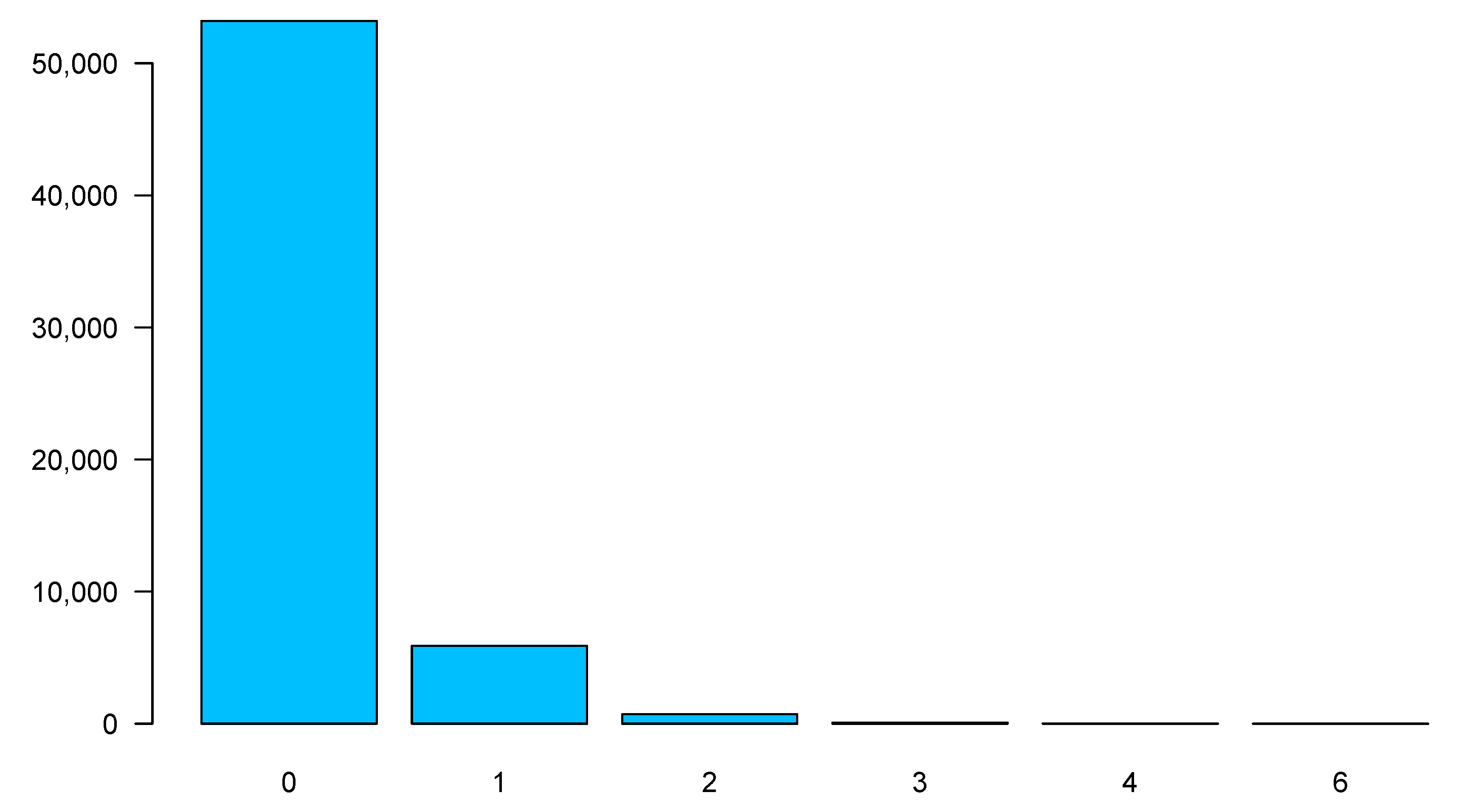
Figure 1 shows the distribution of the number of claims. We can observe that zero claims form a large part of our portfolio.

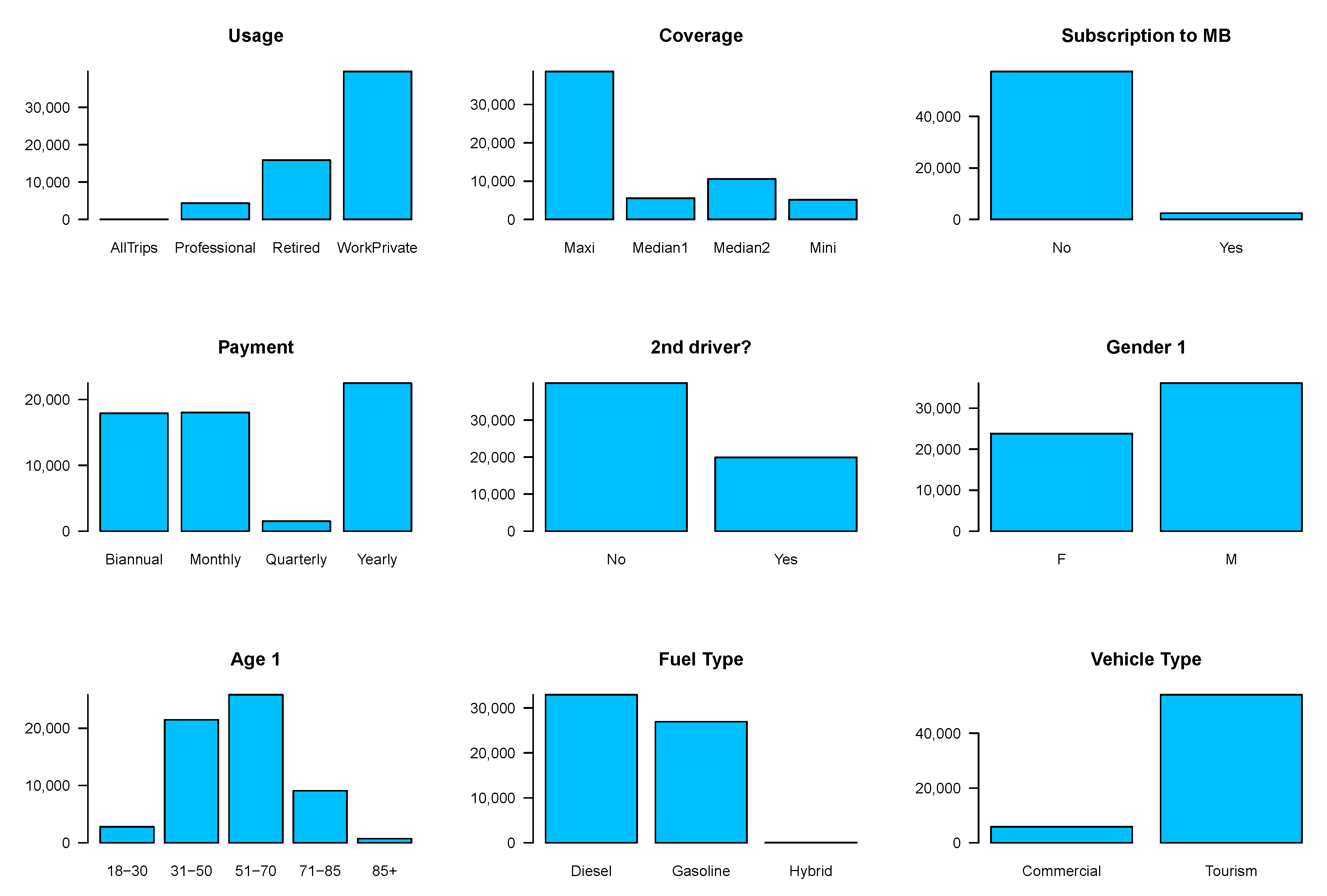
Figure 2 illustrates how policies are distributed across categorical variables. As we can see, most of our policies cover one driver and most of the drivers are men aged between 51 and 70. Our policyholders prefer Maxi and drive tourism cars for work and private purposes. Most of them pay annually and are distributed almost evenly across monthly and biannual payment categories. They have not registered for MB scheme and they use diesel with very few of them using a hybrid car. Next, we see how claims are distributed across categorical variables.

Table 3. Frequency of claims per categorical variables in the training set.

Variables	Categories	Claim Frequency							Total
		0	1	2	3	4	5	6
Policy usage	WorkPrivate	35,248	$\mathrm{3,877}$	450	49	7	0	1	39,632
		$88.94\%$	$9.78\%$	$1.14\%$
	Retired	14,193	$\mathrm{1,462}$	191	20	3	0	0	15,869
		$89.44\%$	$9.21\%$	$1.20\%$
	Professional	$\mathrm{3,729}$	544	76	10	0	0	0	$\mathrm{4,359}$
		$85.55\%$	$12.48\%$	$1.74\%$
	All trips	41	10	1	0	0	0	0	52
		$78.85\%$	$19.23\%$	$1.92\%$
Policy coverage	Maxis	33,459	4,489	600	70	9	0	1	38,628
		$86.62\%$	$11.62\%$	$1.55\%$
	Median 2	9,628	862	82	7	1	0	0	10,580
		$91.00\%$	$8.15\%$	$0.78\%$
	Median 1	$\mathrm{5,122}$	412	32	2	0	0	0	$\mathrm{5,568}$
		$91.99\%$	$7.04\%$	$0.57\%$
	Mini	$\mathrm{5,002}$	130	4	0	0	0	0	$\mathrm{5,136}$
		$97.39\%$	$2.53\%$	$0.08\%$
Subscription to MB	No	50,946	$\mathrm{5,714}$	693	76	10	0	1	57,440
		$88.69\%$	$9.95\%$	$1.21\%$
	Yes	$\mathrm{2,265}$	179	25	3	0	0	0	$\mathrm{2,472}$
		$91.63\%$	$7.24\%$	$1.01\%$
Payment	Yearly	20,094	$\mathrm{2,106}$	263	25	3	0	1	22,492
		$89.34\%$	$9.36\%$	$1.17\%$
	Biannual	15,930	1,746	199	29	3	0	0	17,907
		$88.96\%$	$9.75\%$	$1.11\%$
	Monthly	15,880	$\mathrm{1,875}$	234	23	4	0	0	18,016
		$88.14\%$	$10.41\%$	$1.30\%$
	Quarterly	$\mathrm{1,307}$	166	22	2	0	0	0	$\mathrm{1,497}$
		$87.31\%$	$11.09\%$	$1.47\%$
Policy with 2 drivers	No	35,675	$\mathrm{3,814}$	457	47	6	0	0	39,999
		$89.19\%$	$9.54\%$	$1.14\%$
	Yes	17,536	2,079	261	32	4	0	1	19,913
		$88.06\%$	$10.44\%$	$1.31\%$
Gender 1	Male	32,118	$\mathrm{3,501}$	433	52	4	0	0	36,108
		$88.95\%$	$9.70\%$	$1.20\%$
	Female	21,093	$\mathrm{2,392}$	285	27	6	0	1	23,804
		$88.61\%$	$10.05\%$	$1.20\%$
Age 1	18–30	$\mathrm{2,471}$	299	29	4	0	0	1	$\mathrm{2,804}$
		$88.12\%$	$10.66\%$	$1.03\%$
	31–50	18,961	$\mathrm{2,228}$	256	24	4	0	0	21,473
		$88.30\%$	$10.38\%$	$1.19\%$
	51–70	22,978	$\mathrm{2,479}$	322	40	3	0	0	25,822
		$89.99\%$	$9.60\%$	$1.25\%$
	71–85	8,154	822	105	9	3	0	0	$\mathrm{9,093}$
		$89.67\%$	$9.04\%$	$1.15\%$
	$85+$	647	65	6	2	0	0	0	720
		$89.86\%$	$9.03\%$	$0.83\%$
Vehicle fuel	Diesel	28,605	$\mathrm{3,783}$	475	54	7	0	1	32,925
		$86.88\%$	$11.49\%$	$1.44\%$
	Gasoline	24,565	$\mathrm{2,104}$	241	25	3	0	0	26,938
		$91.19\%$	$7.81\%$	$0.89\%$
	Hybrid	41	6	2	0	0	0	0	49
		$83.67\%$	$12.24\%$	$4.08\%$
Vehicle type	Tourism	47,891	$\mathrm{5,387}$	668	73	10	0	1	54,030
		$88.64\%$	$9.97\%$	$1.24\%$
	Commercial	$\mathrm{5,320}$	506	50	6	0	0	0	$\mathrm{5,882}$
		$90.45\%$	$8.60\%$	$0.85\%$
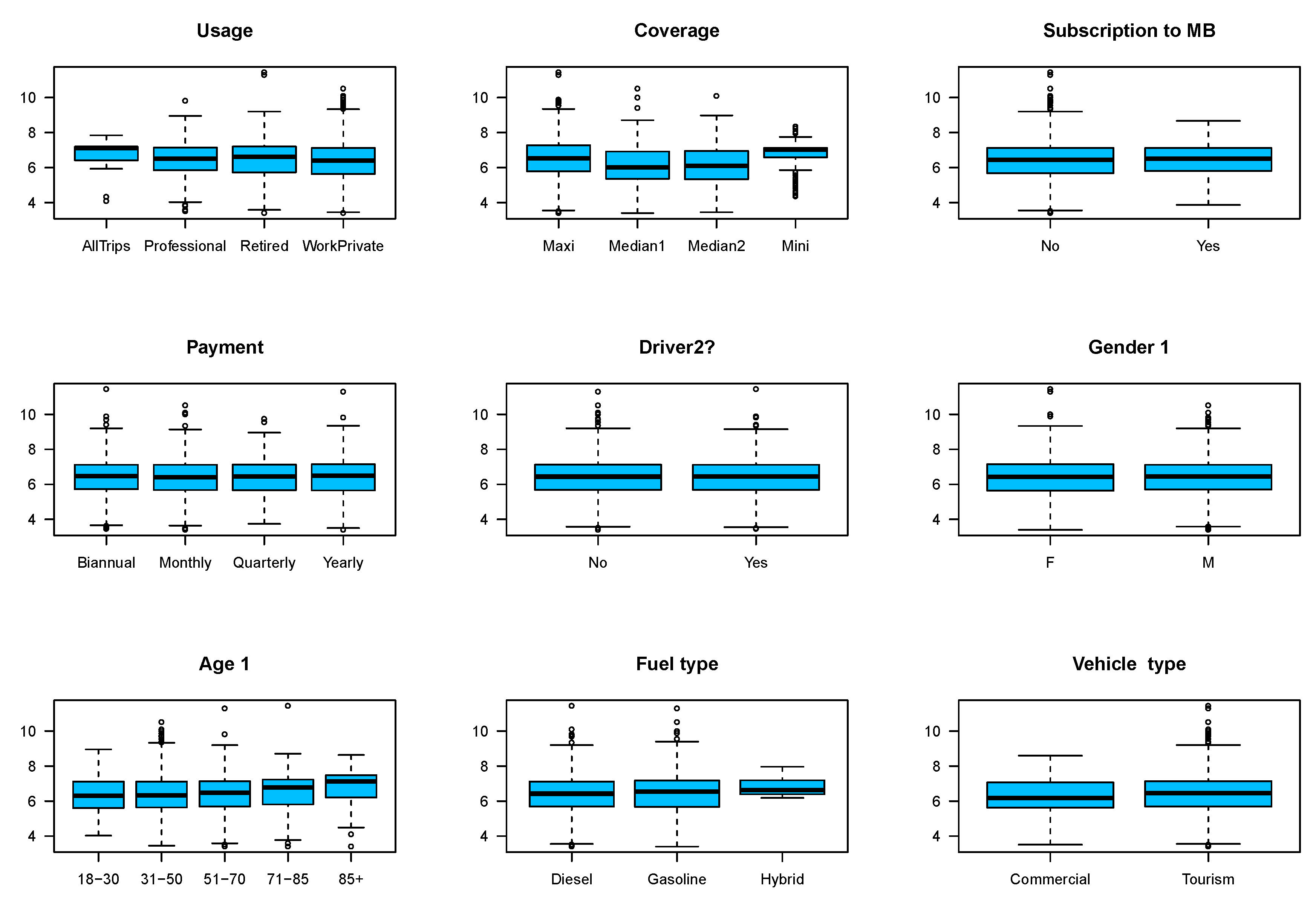
Total		53,211	5,893	718	79	10	0	1	59,912

presents the distribution of the number of claims across different categories. For the variable policy usage, although professional usage forms a small portion of our portfolio, claims under professional group is more than private and retired groups. However, from Figure 3 professional and retired groups have almost the same median loss and except for all trips we can see little difference among policies in this group. Under this insurance, the most comprehensive protection is provided by maxis and as can be expected this may lead to moral hazard. We can see there are more claims under maxis than under other types of coverage. The order of coverage is maxis, median 2, median 1 and mini and unsurprisingly, the percentage of claims reduces in the same order. Under mini, $97.39\%$ of the policies have made zero claims. Perhaps lower coverage is a motivation for policyholders to take more precautious measures. Figure 3 shows the effect of policy coverage on the amounts of claims and as we can see this will be an effective covariate in our model. From Table 3 those policyholders who were willing to subscribe to MB plan are less likely to have an accident. Figure 3 shows that the subscribers are less dispersed than those who have not subscribed. From the regulatory point of view, gender cannot be used as a discriminatory factor. In fact, we can see there is no considerable difference between male’s and female’s number of claims. In Figure 2 the least favourable payment frequency is quarterly payment, but we do not see considerable differences in claim numbers and amounts for different categories of payments. A large number of policies provide coverage only for one driver, but policies with two drivers have a slightly greater chance of making claims. The age of the first driver ranges from 19 to 103. We classify the policyholders in different age groups as 18–30, 31–50, 51–70, 71–85 and 85+. Most of the policyholders are in the range 51–70 and the next largest group is between 31 and 50. Both Table 3 and Figure 3 do not show a significant difference in claims frequency and claim amounts for different age categories and it seems that some categories can be combined together. In fact, in the next section we see that instead of these categories, we use age as a numerical covariate in our models as some categories are not statistically significant.

Most of our policyholders drive gasoline cars and very few of them have hybrid cars.2 According to Table 3, hybrid cars make more claims than gasoline and diesel cars. Most policies cover tourism cars and claims percentage made by this type of cars is more than commercial cars. Our initial analysis suggests that payment frequency and gender are not significant variables and therefore can be removed from our study. In the next section, we will see that they are indeed insignificant and are not included in our final models.

4. Results

In this section, we use statistical software R and package “pscl” to build Poisson, logistic and ZIP models (Zeileis et al. 2008). Our purpose is to estimate the frequency and the probability of claims and compare our results with a ZIP model using Akaike Information Criterion (AIC) and Bayesian Information Criterion (BIC).

Table 4. Regression coefficient of Poisson models.

Coefficients	Model 1: All Variables		Model 2: Stepwise Selection		Model 3: Only Significant
	Estimate	p-Value	Estimate	p-Value	Estimate	p-Value
Intercept	$-2.6883$	<$0.0001$	$-2.5645$	<$0.0001$	$-2.4729$	<$0.0001$
Age 1	$0.0048$	$0.0001$	$0.0048$	$0.0002$	$0.0036$	$0.0026$
Age 2	$-0.0034$	$0.0084$	$-0.0034$	$0.0087$	$-0.0033$	$0.0111$
Female 1	$0.0380$	$0.1251$	$0.0374$	$0.1285$
Driver2?	$0.1790$	$0.0057$	$0.1781$	$0.0060$	$0.1717$	$0.0080$
Situation duration	$-0.0185$	$0.0078$	$-0.0185$	$0.0080$	$-0.0220$	$0.0013$
Bonus	$0.8677$	<$0.0001$	$0.8683$	<$0.0001$	$0.9125$	<$0.0001$
Coverage(Med2)	$-0.1854$	<$0.0001$	$-0.1847$	<$0.0001$	$-0.1877$	<$0.0001$
Coverage(Med1)	$-0.2282$	<$0.0001$	$-0.2280$	<$0.0001$	$-0.2306$	<$0.0001$
Coverage(Mini)	$-1.2611$	<$0.0001$	$-1.2631$	<$0.0001$	$-1.2723$	<$0.0001$
Payment(biannual)	$0.0485$	$0.0919$	$0.0487$	$0.0908$
Payment(quarterly)	$0.1676$	$0.0184$	$0.1681$	$0.0181$
Payment(monthly)	$0.0911$	$0.0018$	$0.0912$	$0.0018$
Subscription to MB	$-0.1586$	$0.0198$	$-0.1587$	$0.0197$	$-0.1675$	$0.01370$
Usage(retired)	$-0.0304$	$0.4331$	$-0.0297$	$0.4433$	$-0.0315$	$0.4146$
Usage(professional)	$0.1536$	$0.0003$	$0.1535$	$0.0002$	$0.1481$	$0.0002$
Usage(all trips)	$0.3451$	$0.2328$	$0.3456$	$0.2321$	$0.3448$	$0.2332$
Duration	$-0.0025$	$0.0969$	$-0.0025$	$0.0978$
Fuel(gasoline)	$-0.2621$	<$0.0001$	$-0.2630$	<$0.0001$	$-0.2607$	<$0.0001$
Fuel(hybrid)	$0.1265$	$0.6896$	$0.1225$	$0.6988$	$0.1196$	$0.70588$
Type(commercial)	$0.0318$	$0.5466$
Din(power)	$0.0022$	$0.0004$	$0.0026$	<$0.0001$	$0.0024$	<$0.0001$
Vehicle age	$-0.0316$	<$0.0001$	$-0.0318$	<$0.0001$	$-0.0332$	<$0.0001$
Vehicle speed	$0.0009$	$0.3967$
Log-likelihood	−23,207		−23,207		−23,216
Degrees of freedom	24		22		17
AIC	46,462		46,458		46,466
BIC	46,678		46,656		46,619
Running time (s)	$0.761$		$7.336$		$0.601$

presents three Poisson regression models with their estimated coefficients and their corresponding p-values. Model 1 is the full model where we consider all the variables from Section 3. However, according to pricing game document, there is a correlation between vehicle cylinder, weight, value, speed and power and in our dataset, some of the entries for weight, value and cylinder are missing. Therefore, we only incorporate speed and power into our models. We build Model 2 using the stepwise selection of variables that can be implemented in R. In Model 3 we only consider variables which are statistically significant at 0.05.

As we can see, some of the coefficients are statistically significant at $0.0001$. For example, the coefficient associated with the Bonus is significant and positive as expected. The bonus represents the percentage of the full premium and a large percentage shows an adverse claims history of a policyholder. The positive sign indicates that as the percentage of the full premium increases, the mean of claims frequency will increase. The coefficients associated with Coverage are negative for all categories and significant. The coefficient of Median 2 shows that the policyholders with this type of coverage have fewer claims than policyholders with Maxi coverage (the reference level). For example, in Model 1, a policyholder with a Median 2 has fewer claims than a policyholder with a Maxi coverage by $exp(-0.1854)=0.83$ and a policyholder with a Mini coverage has fewer claims by $exp(-1.2611)=0.28$. The coefficient of the car’s power, represented by Din, is positive and significant, which indicates that powerful cars are more likely to be involved in an accident and therefore the mean of claims frequency for the owners of the powerful cars is higher. Unlike Ayuso et al. (2019) and Guillen et al. (2019), we found that Vehicle age has a negative impact on the number of claims. In our study, most of the policyholders are middle-aged and more likely to have old cars. In Section 3 we saw that the mean of the vehicle age is 9.56 for all policies and 7.30 for policies with at least one claim. Our portfolio of middle-aged policyholders also affects the sign of the coefficient associated with Age 1. Our dataset includes drivers as old as 103. Therefore, it seems reasonable to find a positive impact of age on the mean of the number of claims. In Model 1 the coefficients which are not significantly different from zero include Female 1, car usage for Retired and All trips, Hybrid fuel, Type and Speed. The coefficient of Professional usage indicates that Professional usage increases the mean of claims frequency compared to Work and private usage (the reference level) by $exp\left(0.1536\right)=1.17$. This is in line with Table 3 that policies for professional purposes make more claims. We obtain similar results for gasoline cars as in Table 3. Owners of Gasoline cars have fewer claims than owners of Diesel cars by $exp(-0.2621)=0.77$. We can see that the coefficient associated with Driver2 is positive. This seems reasonable as a policy that covers two drivers is more likely to make claims. The coefficient of Age 2 is negative. One interpretation can be that the average age of the second drivers is lower than the average age of the first drivers. However, in Section 3, we saw that driver age 2 is not significantly different for policies with claims and policies without claims. The coefficients associated with Duration and Policy duration are both negative. This implies that more experienced policyholders make fewer claims and also the more stable a policy is, the lower the mean of the number of claims. The coefficient of subscription to MB is negative and therefore this variable reduces the mean of claims frequency. Perhaps those who are willing to be monitored by telematics technology are more confident about their driving behaviour. We saw in the previous section that payment frequency is not a significant variable. As we can see, their corresponding p-values for some categories in models 1 and 2 are not significant at $0.05$ and therefore we have removed them from Model 3. However, we decided to keep the variable Usage, although not all categories are significant at 0.05, as we found in the previous section that it is effective on the number of claims. Among our three models, Model 2 has the lowest AIC and Model 3 has the lowest BIC. As we can see, the computation time for Model 2 is longer than the other two models. The reason is that the stepwise algorithm examines different models to find the one with the smallest AIC.

Table 5. Regression coefficients of logistic models.

Coefficients	Model 1: All variables		Model 2: Stepwise Selection		Model 3: Only Significant
	Estimate	p-Value	Estimate	p-Value	Estimate	p-Value
Intercept	$-2.6571$	<$0.0001$	$-2.5321$	<$0.0001$	$-2.4255$	<$0.0001$
Age 1	$0.0043$	$0.0036$	$0.0038$	$0.0066$	$0.0032$	$0.0226$
Age 2	$-0.0048$	$0.0011$	$-0.0047$	$0.0013$	$-0.0047$	$0.0013$
Female 1	$0.0441$	$0.1198$	$0.0428$	$0.1275$
Driver2?	$0.2410$	$0.0012$	$0.2363$	$0.0014$	$0.2340$	$0.0016$
Situation duration	$-0.0234$	$0.0027$	$-0.0248$	$0.0013$	$-0.0265$	$0.0006$
Bonus	$0.9017$	<$0.0001$	$0.9151$	<$0.0001$	$0.9447$	<$0.0001$
Coverage(Med2)	$-0.1814$	<$0.0001$	$-0.1786$	<$0.0001$	$-0.1832$	<$0.0001$
Coverage(Med1)	$-0.2111$	$0.0005$	$-0.2061$	$0.0007$	$-0.2132$	$0.0004$
Coverage(Mini)	$-1.2481$	<$0.0001$	$-1.2438$	<$0.0001$	$-1.2589$	<$0.0001$
Payment(biannual)	$0.0522$	$0.1121$	$0.0490$	$0.1335$
Payment(quarterly)	$0.1852$	$0.0240$	$0.1883$	$0.0217$
Payment(monthly)	$0.0939$	$0.0049$	$0.0936$	$0.0051$
Subscription to MB	$-0.2014$	$0.0088$	$-0.2038$	$0.0080$	$-0.2098$	$0.0063$
Usage(retired)	$-0.0180$	$0.6847$	$-0.0149$	$0.7364$	$-0.0203$	$0.6455$
Usage(professional)	$0.1691$	$0.0007$	$0.1733$	$0.0002$	$0.1664$	$0.0004$
Usage(all trips)	$0.4841$	$0.1577$	$0.4856$	$0.1563$	$0.4835$	$0.1577$
Duration	$-0.0019$	$0.2708$
Fuel(gasoline)	$-0.2885$	<$0.0001$	$-0.2914$	<$0.0001$	$-0.2875$	<$0.0001$
Fuel(hybrid)	$0.0707$	$0.8560$	$0.0691$	$0.8592$	$0.0598$	$0.8778$
Type(commercial)	$0.0462$	$0.4402$
Din(power)	$0.0022$	$0.0019$	$0.0027$	<$0.0001$	$0.0025$	<$0.0001$
Vehicle age	$-0.0336$	<$0.0001$	$-0.0336$	<$0.0001$	$-0.0332$	<$0.0001$
Vehicle speed	$0.0010$	$0.4404$
Log-likelihood	−20,292		−20,293		−20,299
Degrees of freedom	24		21		17
AIC	40,632		40,628		40,633
BIC	40,848		40,817		40,785
Running time (s)	$0.634$		$31.611$		$0.431$

presents three logistic models with their coefficients and the corresponding p-values. Similar to Table 4, Model 1 includes all variables, Model 2 is based on the stepwise algorithm and Model 3 only includes significant variables. The interpretation of the coefficients in logistic regression is similar to Poisson regression and as we can see, the signs of the coefficients are the same. The only difference is that in logistic regression we look at the impact of variables on the odds of the occurrence of claims. So, for example, the interpretation of the coefficient associated with Bonus is that, the greater the percentage of the full premium (adverse claims history) is, the higher the odds of the occurrence of the claims for the coefficient associated with professional usage; we can say that the odds of the occurrence of claims for policyholders with professional usage increases by $exp\left(0.1691\right)=1.18$ as opposed to policyholders with work and private usage. For the negative coefficient associated with subscription to MB, we can say that the odds of the occurrence of claims fall for a policyholder who joins this scheme. Other variables can be similarly interpreted. Model 2 is built by examining different models and finding the one with the lowest AIC. All variables in this model are the same as the variables in stepwise Poisson regression except for duration which is not included in stepwise logistic regression. For Model 3 we again remove all variables with a p-value greater than 0.05. In addition, we do not include payment frequency as this has been proved to be insignificant in Section 3. As we can see, Model 2 has the smallest AIC and Model 3 has the smallest BIC. Further, the computation time for the stepwise algorithm is longer than the stepwise Poisson regression model.

When building a model, it is important to consider the underlying assumptions. For example, to fit a ZIP model to our data, we first need to test for the presence of over-dispersion. One approach is to fit a quasi-Poisson and to determine the dispersion parameter, i.e., $\theta$ in Var$\left(y\right)=\theta$ E$\left[y\right]$. In our case, using only significant variables from Table 4 and Table 5, the dispersion parameter is $1.1$. Alternatively, we can fit NB regression and compare our new model with Poisson regression. In our case, AIC and BIC for NB regression are 46,184 and 46,346, respectively, which are lower than AIC and BIC for the Poisson regression. Now, since we have the problem of over-dispersion and excess zeros, we can fit a ZIP model to our data.

Table 6. Regression coefficients of zero-inflated Poisson (ZIP) models.

Coefficients	Model 1 *			Model 2 *			Model 3 *
	Estimate	p-Value		Estimate	p-Value		Estimate	p-Value
Poisson (count) part
Intercept	−2.2750	<$0.0001$		−2.1404	<$0.0001$		−2.0736	<$0.0001$
Age 1	0.0066	0.0513		0.0063	0.0542		0.0046	0.1347
Age 2	0.0012	0.6647		0.0013	0.6290		0.0019	0.4998
Female 1	−0.0448	0.4746		−0.0479	0.4324
Driver2?	−0.0473	0.7366		−0.0536	0.6972		−0.0809	0.5584
Situation duration	−0.0009	0.0194		−0.0017	0.9282		−0.0011	0.9558
Bonus	0.5787	0.2021		0.5953	0.2068		0.5433	0.2026
Coverage(Med2)	−0.3670	0.0006		−0.3734	0.0004		−0.3646	0.0006
Coverage(Med1)	−0.4294	0.0022		−0.4231	0.0022		−0.4269	0.0024
Coverage(Mini)	−1.0487	0.0017		−1.0599	0.0016		−1.1031	0.0007
Payment(biannual)	−0.0691	0.3318		−0.0668	0.3472
Payment(quarterly)	-0.0569	0.7525		−0.0452	0.8002
Payment(monthly)	0.0091	0.8961		0.0137	0.8427
Subscription to MB	0.0596	0.7580		0.0462	0.8099		0.0126	0.9486
Usage(retired)	−0.0623	0.5523		−0.0623	0.5455		−0.0538	0.6006
Usage(professional)	0.0723	0.5491		0.0710	0.5063		0.0952	0.3725
Usage(all trips)	0.2543	0.6523		0.2375	0.6765		−0.0332	0.9544
Duration	−0.0043	0.2948		−0.0025	0.1145
Fuel(gasoline)	−0.0346	0.6549		−0.0387	0.6228		−0.0759	0.3854
Fuel(hybrid)	0.6976	0.2553		0.7050	0.2500		0.6366	0.3302
Type(commercial)	0.0284	0.8457
Din(power)	0.0023	0.3055		0.0026	0.1207		0.0024	0.3063
Vehicle age	0.0024	0.7925		0.0032	0.1207		0.0063	0.4799
Vehicle speed	0.0010	0.7557
Zero-inflation part
Intercept	−0.5544	0.6449		−0.4634	0.6883		−0.4819	0.6826
Age 1	0.0040	0.5922		0.0032	0.6558		0.0020	0.7736
Age 2	0.0108	0.0653		0.0111	0.0546		0.0121	0.0356
Female 1	−0.1962	0.1572		−0.2020	0.1358
Driver2?	−0.5491	0.0892		−0.5633	0.0748		−0.6165	0.0522
Situation duration	0.0331	0.3289		0.0309	0.3575		0.0387	0.2442
Bonus	−0.8651	0.4958		−0.8200	0.5308		−1.0637	0.3802
Coverage(Med2)	−0.3798	0.1014		−0.3932	0.0848		−0.3595	0.1139
Coverage(Med1)	−0.4030	0.1541		−0.3871	0.1601		−0.3847	0.1645
Coverage(Mini)	0.2803	0.5949		0.2610	0.6222		0.2052	0.6923
Payment(biannual)	−0.2596	0.0910		−0.2547	0.0963
Payment(quarterly)	−0.5661	0.2637		−0.5354	0.2798
Payment(monthly)	−0.1721	0.2518		−0.1615	0.2751
Subscription to MB	0.4226	0.2041		0.3978	0.2310		0.3560	0.3030
Usage(retired)	−0.0775	0.7250		−0.0783	0.7177		−0.0533	0.8043
Usage(professional)	−0.2215	0.4672		−0.2273	0.4063		−0.1510	0.5703
Usage(all trips)	−0.3050	0.8550		−0.3668	0.8345		−1.8681	0.7405
Duration	−0.0040	0.6448
Fuel(gasoline)	0.5066	0.0017		0.5002	0.0021		0.4090	0.0236
Fuel(hybrid)	114.80	0.1984		116.60	0.1890		1.0632	0.2829
Type(commercial)	0.0041	0.9901
Din(power)	0.0000	0.9944		-0.0000	0.9959		−0.0002	0.9627
Vehicle age	0.0696	<$0.0001$		0.0712	<$0.0001$		0.0756	<$0.0001$
Vehicle speed	0.0006	0.9258
Log-likelihood	−23,044			−23,045			−23,054
Degrees of freedom	48			43			34
AIC	46,184			46,175			46,177
BIC	46,616			46,563			46,482
Running time (s)	16.719			$18.81$			$13.951$

* Model 1: full model; Model 2: based on the variables of stepwise models in Table 4 and Table 5; Model 3: based on the variables of only significant models in Table 4 and Table 5.

shows the estimated coefficients and their p-values for the Poisson (count) part and zero-inflated part of three ZIP models. Model 1 is the full model where we consider the variables of the full model in Table 4 for the count part and the variables of the full model in Table 5 for the zero-inflated part. As we can see, most variables are not significantly different from zero. If we consider the significant level of 0.1, the coefficient associated with Age 1 is positive as in Table 4 and statistically significant in the count part. In addition, the coefficient associated with Age 2 is positive and significant in the zero-inflated part, but not in the count part. From Section 3, we know that the second divers are younger than the first drivers. Therefore, we can claim that in this group older drivers are more likely to have zero claims. The coefficient of situation duration in the count part is negative and significant as in Table 4 with the same interpretation. The coefficients associated with coverage are significant at 0.01 in the count part with the identical signs as in Table 4, but they are not significant in the zero-inflated part. The interpretation is that the mean frequency of claims for policyholders covered under, for example, Mini coverage is less than the policyholders covered under Maxi coverage by $exp(-1.0487)=0.35$.

The coefficient of fuel (gasoline) is positive and significant which indicates that the odds of zero claims for drivers of gasoline cars increases by $exp\left(0.5066\right)=1.66$ as opposed to drivers of diesel cars. Further, in the zero-inflated part, the coefficient of Driver2? is negative and significant. Therefore, a policy with two drivers is less likely to have zero claims, in other words, a policy with the 2nd driver is more likely to be involved in an accident and to make a claim. The associated coefficient of vehicle age is positive and significantly different from zero in the zero-inflated part, which is in line with our findings for Poisson and logistic models that it is more likely for the owners of older cars to have zero claims. All other variables including subscription to MB are not significantly different from zero. The variables of Model 2 in the count and zero-inflated part come from the variables of stepwise models in Table 4 and Table 5, respectively. The coefficients have the same sign and therefore similar interpretation as in Model 1. Again the coefficient of subscription to MB is not significantly different from zero. Model 3 can be built using the variables of the models that contain only significant variables in Table 4 and Table 5. Coverage in the count part and Age 2, Driver2?, fuel and vehicle age in the zero-inflated part are all significantly different from zero. In Table 6 the signs of some of the coefficients do not conform to Table 4 and Table 5. For example, subscription to MB is positive both in the count part and in the zero-inflated part. Since such coefficients are not statistically significant, we can conclude that they are not significantly different from zero. Comparing AIC and BIC of these three models, we can see that the smallest AIC can be obtained by Model 2 where the variables come from stepwise models in Table 4 and Table 5 and the smallest BIC by Model 3. In addition, AIC has considerably improved for ZIP models compared to Poisson models in Table 4. In the next section, we show that the prediction of zero claims by ZIP is considerably better than Poisson regression.

5. Validation

In this section, we use our validation set to compare the predictability of the models discussed in Section 4.

Table 7. Prediction of the probability and the number of zero claims by our models.

			Prob Zero Claims: Individual 1 **	Prob Zero Claims: Individual 2 ***	Total No. of Zero Claims	Total No. of Non-Zero Claims
Observed value			0	1	35,772	4316
Poisson	Full model		0.9016	0.8358	35,361.44	4726.56
	Stepwise		0.9019	0.8350	35,361.27	4726.73
	Significant		0.9019	0.8410	35,360.50	4727.50
Logistic	Full model		0.9097	0.8475	35,606.88	4481.12
	Stepwise		0.9091	0.8480	35,606.95	4481.05
	Significant		0.9102	0.8512	35,606.62	4481.38
ZIP	Model 1 *	Count	0.1024	0.1778	35,602	4486
		Zero	0.9104	0.8446
	Model 2 *	Count	0.1016	0.1785	35,601.27	4486.74
		Zero	0.9113	0.8440
	Model 3 *	Count	0.1020	0.1710	35,601.06	4486.94
		Zero	0.9113	0.8495

* Model 1: full model; Model 2: based on the variables of stepwise models in Table 4 and Table 5; Model 3: based on the variables of only significant models in Table 4 and Table 5. ** An 85-year-old male policyholder with biannual maxi coverage and bonus of 0.5 for retired usage. He had this policy for 29 years and changed it nine years ago. He has not registered for MB and owns a 10-year old tourism car with gasoline, the din of 98 and max speed of 182. *** A 54-year-old male with monthly maxi coverage and bonus of 0.5 for private usage. The 2nd driver is a 56-year-old female. The policy was written six years ago and was modified two years ago. It covers a two-year-old tourism car with diesel and din of 75 and max speed of 163. It is not part of MB scheme.

presents the predicted number of zero and non-zero claims by our models in Section 4. In this table, individual 1 refers to an 85-year-old male policyholder with a maxi policy that pays biannually with the bonus (percentage of the full premium) of 0.5. He holds this policy for retired usage, for 29 years and has not signed to MB scheme. The policy was modified nine years ago. He owns a 10-year-old tourism car with gasoline, the din of 98 and max speed of 182. In year 0, this policyholder has not made any claim and the probability of zero claims predicted by Poisson regression according to full model is $exp(-0.1036)$ where 0.1036 is the estimated parameter $\lambda$ and the probability of zero claims predicted by logistic regression is $1-0.0903$ where $0.0903$ is the estimated $\pi =$ Pr$(y=1)$. Prediction of zero claims by ZIP is 0.9104. Individual 2 is a male policyholder with a maxi policy. This policy covers two drivers aged 54 and 56 and has been held for six years and been modified two years ago with a bonus of $0.5$ and monthly premium payment. The policyholder owns a two-year old tourism car with diesel for work and private purposes with the din of 75 and max speed of 163. The estimated parameter by Poisson regression is $\lambda =0.1794$ and by logistic regression is $\pi =0.1525$. As we can see, the count part of ZIP for the two policyholders is very close to the estimated value of Poisson regression. If we add the probability of zero claims in all these models, we can approximate the number of zero claims. Results show that ZIP models considerably outperform Poisson regression and logistic regression performs better than ZIP models in predicting zero claims. Further, we can see that there is a slight difference between predictions made by full models, stepwise models and the models with only significant variables.

6. Conclusions

We have divided our dataset into training and validation sets. Using our training set, we have developed three models and compared our models according to their AIC and BIC values. We found that type of coverage, vehicle age and fuel are statistically significant in most of our models. We then validated our models and showed that a ZIP model can predict the frequency of claims better than a Poisson regression. Further, we have shown that if we are just concerned about the number of zero and non-zero claims, logistic regression can even outperform a ZIP model. In fact, logistic regression is a one layer neural network and there is a scope to extend our study to a more generalised form of logistic regression for future research. We saw that the policyholders who were willing to be monitored by telematics devices are less likely to make a claim. A thorough study of the policyholders’ behaviour before and after being monitored by telematics devices can be another area of future research. Given the current concern regarding climate change and sustainability, the possibility of the inclusion of fuel consumption into a pricing model may be considered in the future (Tselentis et al. 2017).

References

- Ayuso, Mercedes, Montserrat Guillen, and Jens Perch Nielsen. 2019. Improving automobile insurance ratemaking using telematics: incorporating mileage and driver behaviour data. Transportation 46: 735–52. [Google Scholar] [CrossRef]
- Boucher, Jean-Philippe, Michel Denuit, and Montserrat Guillén. 2007. Risk classification for claim counts. North American Actuarial Journal 11: 110–31. [Google Scholar] [CrossRef]
- Boucher, Jean-Philippe, Michel Denuit, and Montserrat Guillen. 2009. Number of accidents or number of claims? An approach with zero-inflated Poisson models for panel data. The Journal of Risk and Insurance 76: 821–46. [Google Scholar] [CrossRef]
- Boucher, Jean-Philippe, Steven Côté, and Montserrat Guillen. 2017. Exposure as duration and distance in telematics motor insurance using generalized additive models. Risks 5: 54. [Google Scholar] [CrossRef]
- Cantoni, Eva, and Marie Auda. 2018. Stochastic variable selection strategies for zero-inflated models. Statistical Modelling 18: 3–23. [Google Scholar] [CrossRef]
- Chen, Kun, Rui Huang, Ngai Hang Chan, and Chun Yip Yau. 2019. Subgroup analysis of zero-inflated Poisson regression model with applications to insurance data. Insurance: Mathematics and Economics 86: 8–18. [Google Scholar] [CrossRef]
- Chowdhury, Shrabanti, Saptarshi Chatterjee, Himel Mallick, Prithish Banerjee, and Broti Garai. 2019. Group regularization for zero-inflated poisson regression models with an application to insurance ratemaking. Journal of Applied Statistics 46: 1567–81. [Google Scholar] [CrossRef]
- Dutang, Christophe, and Arthur Charpentier. 2019. CASdatasets: Insurance Datasets. Available online: http://dutangc.free.fr/pub/RRepos/web/CASdatasets-index.html (accessed on 15 March 2019).
- Fauzan, Muhammad Arief, and Hendri Murfi. 2018. The accuracy of XGBoost for insurance claim prediction. International Journal of Advances in Soft Computing and Its Applications 10: 159–71. [Google Scholar]
- Ferreira, Joseph, and Eric Minikel. 2012. Measuring per mile risk for pay-as-you-drive automobile insurance. Transportation Research Record: Journal of the Transportation Research Board 2297: 97–103. [Google Scholar] [CrossRef]
- Frees, Edward W., Richard A. Derrig, and Glenn Meyers. 2014. Predictive Modeling Applications in Actuarial Science, Volume I: Predictive Modeling Techniques. New York: Cambridge University Press. [Google Scholar]
- Frees, Edward W., Richard A. Derrig, and Glenn Meyers. 2016. Predictive Modeling Applications in Actuarial Science, Volume II: Case Studies in Insurance. New York: Cambridge University Press. [Google Scholar]
- Gao, Guangyuan, Shengwang Meng, and Mario V. Wüthrich. 2019. Claims frequency modeling using telematics car driving data. Scandinavian Actuarial Journal 2019: 143–62. [Google Scholar] [CrossRef]
- Guillen, Montserrat, Jens Perch Nielsen, Mercedes Ayuso, and Ana M. Pérez-Marín. 2019. The use of telematics devices to improve automobile insurance rates. Risk Analysis 39: 662–762. [Google Scholar] [CrossRef] [PubMed]
- Haberman, Steven, and Arthur E. Renshaw. 1996. Generalized linear models and actuarial science. The Statistician 45: 407–36. [Google Scholar] [CrossRef]
- Lambert, Diane. 1992. Zero-inflated Poisson regression, with an application to defects in manufacturing. Technometrics 34: 1–14. [Google Scholar] [CrossRef]
- Lee, Andy H., Mark R. Stevenson, Kui Wang, and Kelvin K. W. Yau. 2002. Modeling young driver motor vehicle crashes: Data with extra zeros. Accident Analysis and Prevention 34: 515–21. [Google Scholar] [CrossRef]
- Lemaire, Jean, Sojung Carol Park, and Kili C. Wang. 2015. The use of annual mileage as a rating variables. Astin Bulletin 46: 39–69. [Google Scholar] [CrossRef]
- Liu, Feng, and David Pitt. 2017. Application of bivariate negative binomial regression model in analysing insurance count data. Annals of Actuarial Science 11: 390–411. [Google Scholar] [CrossRef] [Green Version]
- McCullagh, Peter, and John A. Nelder. 1998. Generalized Linear Models. London: Chapman and Hall. [Google Scholar]
- Murphy, Kevin P. 2012. Machine Learning—A Probabilistic Perspective. Cambridge: The MIT Press. [Google Scholar]
- Perumean-Chaney, Suzanne E., Charity Morgan, David McDowall, and Inmaculada Aban. 2013. Zero-inflated and overdispersed: What’s one to do? Journal of Statistical Computation and Simulation 83: 1671–83. [Google Scholar] [CrossRef]
- Spedicato, Giorgio Alfredo, Christophe Dutang, and Leonardo Petrini. 2018. Machine learning methods to perform pricing optimization. A comparison with standard GLMs. Variance, Casualty Actuarial Society 12: 69–89. [Google Scholar]
- Tang, Yanlin, Liya Xiang, and Zhongyi Zhu. 2014. Risk factor selection in rate making EM adaptive LASSO for zero-inflated Poisson regression models. Risk Analysis 34: 1112–27. [Google Scholar] [CrossRef]
- Tselentis, Dimitrios I., George Yannis, and Eleni I. Vlahogianni. 2017. Innovative motor insurance schemes: A review of current practices and emerging challenges. Accident Analysis and Prevention 98: 139–48. [Google Scholar] [CrossRef]
- Verbelen, Roel, Katrien Antonio, and Gerda Claeskens. 2018. Unraveling the predictive power of telematics data in car insurance pricing. Journal of the Royal Statistical Society: Series C (Applied Statistics) 67: 1275–304. [Google Scholar] [CrossRef]
- Weerasinghe, K. P. M. L. P., and M. C. Wijegunasekara. 2016. A comparative study of data mining algorithms in the prediction of auto insurance claims. European International Journal of Science and Technology 5: 47–54. [Google Scholar]
- Wilson, Paul, and Jochen Einbeck. 2018. A new and intuitive test for zero modification. Statistical Modelling. [Google Scholar] [CrossRef]
- Yip, Karen C. H., and Kelvin K. W. Yau. 2005. On modeling claim frequency data in general insurance with extra zeros. Insurance: Mathematics and Economics 36: 153–63. [Google Scholar] [CrossRef]
- Zeileis, Achim, Christian Kleiber, and Simon Jackman. 2008. Regression models for count data in R. Journal of Statistical Software 27: 1–25. [Google Scholar] [CrossRef]