Bail-In or Bail-Out? Correlation Networks to Measure the Systemic Implications of Bank Resolution

Abstract

We propose a statistical measure, based on correlation networks, to evaluate the systemic risk that could arise from the resolution of a failing or likely-to-fail financial institution, under three alternative scenarios: liquidation, private recapitalization, or bail-in. The measure enhances the observed CDS spreads with a risk premium that derives from contagion effects across financial institutions. The empirical findings reveal that the recapitalization of a distressed bank performed by the other banks in the system and the bail-in resolution minimize the potential losses for the banking sector with respect to the liquidation scenario, thus posing limited systemic risks. A closer comparison between the private intervention recapitalization and the bail-in tool shows that the latter slightly reduces contagion effects with respect to the private intervention scenario.

1. Introduction and Background

1.1. Measuring Systemic Risk in the Banking Sector

Measuring systemic risk in the banking sector is problematic, because of the high number of dimensions to be included. Accordingly, different econometric models have been applied to a variety of data, in different geographical regions and periods. We can classify systemic risk models into three main categories: bivariate models (Acharya et al. 2010, 2012; Adrian and Brunnermeier 2016; Brownlees and Engle 2012); causal models (Abedifar et al. 2017; Betz et al. 2014; Duffie and Lando 2001; Duprey et al. 2018; Hautsch et al. 2015; Koopman et al. 2012; Lando and Nielsen 2010), and network models (Ahelegbey et al. 2015; Battiston et al. 2012; Billio et al. 2012; Diebold and Yilmaz 2014; Giudici and Spelta 2016; Giudici and Parisi 2018; Giudici et al. 2017; Lorenz et al. 2009). While the first two explicitly deal with the time-varying dimension, the latter focuses on the cross-sectional dimension.

The aim of this paper is two-fold: first, to contribute to the literature on systemic risk measurement through a network-based methodology able to consider both the time and the cross-sectional dimension; second, to show the beneficial effects of the bail-in tool, expressed in terms of decreased potential losses for taxpayers, in case of a simulated shock in the banking sector.

The Corporate Default Swap (CDS) spread of an institution at time $t-1$ is often used as a good predictor of the default probability of the same institution at time t: in an efficient market, CDS prices adjust to reflect all the available information. However, CDS spreads may not quickly adjust for multivariate dependencies, especially during banking crisis times, when cascade effects are often very fast and highly non-linear (see, e.g., Avdjiev et al. (2018)). To overcome this problem, we propose to improve the predictive accuracy of CDS spreads, by adding to them a risk premium derived from their correlations.

1.2. The Systemic Effects of Bank Resolution

While the relative importance of the shadow banking sector has been constantly increasing in the last few years, banks can still be considered as the most relevant contributors to systemic risk. For this reason, in the aftermath of the global financial crisis, policies aimed at monitoring and supervising systemic risk arising from the banking sector have been developed in several countries, within newly-established macro-prudential frameworks.

The European Union has introduced the 2014/59/EU directive, known as the Bank Recovery and Resolution Directive (BRRD), and the Single Resolution Mechanism Regulation (SRMR), which became fully operational in January 2016. In particular, while both the BRRD and the SRMR pose the foundation for the finalization of Pillar 2 of the Banking Union, they have different scopes of application, since the BRRD applies to all EU Member States and confers new powers to resolution authorities in the EU, while the SRMR unifies the resolution of non-viable financial institutions within the Banking Union. Both the Directive and the Regulation are based on the same basic principles to be adopted when restructuring a financial institution, which prescribe the allocation of losses and costs among banks’ shareholders and creditors, rather than on taxpayers.

Before the introduction of the BRRD and the SRMR, when a bank was deemed failing or likely-to-fail, national resolution authorities could essentially choose between liquidation, with high costs for all involved stakeholders (shareholders, bondholders, depositors, borrowers) and a public bail-out, with high costs for taxpayers, relevant moral hazard problems, and vicious sovereign-bank loops (see, e.g., Halaj et al. (2018)).

The BRRD framework proposes four alternative solutions to deal with a failing or likely-to-fail bank: among them, we will focus on the bail-in tool, which imposes on private creditors an ordered reconstruction of the bank, protecting taxpayers, while, at the same time, avoiding the extreme consequences that would occur in case of liquidation. According to Article 32 of the BRRD, a resolution action can be adopted if, and only if, some preliminary conditions are met: (a) the bank has been assessed as failing or likely to fail; (b) no alternative private interventions, nor supervisory interventions, would prevent such failure; (c) a resolution action is necessary in the public interest. The decision of whether a bank can be classified as failing or likely-to-fail (Condition (a)) is a competence of the supervisory authority (the European Central Bank (ECB) for significant institutions). The Single Resolution Board (SRB) of the SRMR, however, has the power of making this decision if the ECB does not, and it has the responsibility to determine whether Conditions (b) and (c) are satisfied.

Our aim is to provide a methodology that can measure the consequences resulting from alternative decisions, involving both the ECB and the SRB, in case one financial institution is failing: bail-in, private intervention, and liquidation. We remark that with “private intervention”, we mean that the failing bank is recapitalized (and totally or partially acquired) by other banks or private companies, even without a supervisory action:1 this marks a substantial difference with the public intervention, or bail-out, where the bank is totally rescued through the use of public funds. This latter possibility is not considered in our analysis, as the BRRD does not explicitly take it into account (apart from exceptional circumstances that, for instance, might allow extraordinary recapitalization actions).

While there is reference literature focusing on the policy debate about the bail-in as opposed to the bail-out (see, e.g., Beck et al. (2017), and the references therein), there is very limited literature on the systemic implications of banks’ resolution, which in our view could be of great support to supervisors, resolution authorities, and policy experts. An exception is the recent paper by Halaj et al. (2018), who analyzed the implications of bail-in on the largest 26 banks in the Euro area by using confidential European Central Bank data on common exposures. We follow Halaj et al. (2018), but, rather than confidential bank balance-sheet data, we employ market-based data, which, albeit less precise, are transparent and easily accessible and reproducible.

To measure the systemic implications of bank resolution, we will examine the evolution of the Corporate Default Swap (CDS) spreads for a set of financial institutions. The use of multivariate CDS spread data will allow us to develop a correlation network model able to identify if and how the distress of one bank might propagate to other institutions and to measure the consequences it would produce in terms of losses for the banking sector. Specifically, the model will be employed to compare the potential losses that could occur under three possible scenarios: (a) liquidation, if the distressed institution no longer meets the minimum capital requirements and is not deemed systemic; (b) private intervention, if the distressed institution is rescued through a partial or total acquisition of the bank by other institutions; (c) bail-in, if the distressed institution no longer meets the minimum capital requirements, but is considered systemic.

Under Scenario (a), the liquidation of the distressed bank implies an immediate shock on the default probabilities and the potential losses of the other banks. However, after some time, the banking system would reach a new steady state without the defaulted bank and, thus, be less affected by contagion risk.

Under Scenario (b), the distressed bank does not default and, consequently, does not immediately affect the other financial institutions. However, the bank remains in the system so that all the other banks in the network would keep suffering contagion risk. Furthermore, all banks that decide to participate in the recapitalization would become even more exposed to the failing bank, thus increasing their potential losses.

Finally, under Scenario (c) the distressed bank remains in the system as under Scenario (b); in this case, contagion risk would derive not only from the persistence of a highly risky bank in the system, but also from the loss sharing that would be imposed on the other banks as creditors of the bailed-in bank.

Our proposed correlation network model will compare the consequences on the financial system of the three alternative scenarios. It will consider two different viewpoints: (a) each single bank’s perspective and (b) the system perspective. In the former, the model will focus on each bank’s loss distribution, under the three scenarios, with the aim of providing to each bank guidelines to decide whether it is convenient to take part in a private intervention or not. In the latter, the model will focus on the potential losses for the entire banking system under the three scenarios, with the aim of providing supervisory authorities and policy makers guidelines to decide which resolution action to implement.

The model will be first applied to the stylized case of three banks: two safe banks (one larger than the other) and one distressed bank (much smaller than the other two). Within this context, we will evaluate the reduction in the potential losses of the safe banks in the case of a private intervention, relative to the potential losses that would occur in case the distressed bank is liquidated. Our results reveal that, from a bank’s viewpoint, a private recapitalization should be generally preferred to the liquidation scenario. Such a preference would be even higher if the safe banks in the system are relatively small.

We will then apply our methodology to the Italian banking system. In our view, this is an interesting case study, as in early 2016, Italian banks organized the creation of an equity fund, called Atlante, which includes, among its main objectives, the recapitalization of distressed financial institutions. Each bank has decided, on a voluntary basis, whether to allocate capital to the Atlante fund: as a result, two medium-sized lenders, Banca Popolare di Vicenza and Veneto Banca, which had been found strongly undercapitalized by the European Central Bank, have been recapitalized with the help of most of the banks in the system. One year later, both banks were split into a good bank, acquired by Intesa San Paolo, and a bad bank, liquidated through national insolvency procedures. A similar intervention occurred for three other banks: Banca Etruria, Banca Marche, and CariChieti, which had been found extremely undercapitalized before the BRRD became fully operative. They were split into a good bank, sold to Unione Banche Italiane (UBI) in 2017, and a bad bank, sold to the Atlante fund. A different discussion has involved Monte dei Paschi di Siena, whose larger size suggested a precautionary recapitalization through the extraordinary use of public money (approved by the European Commission in 2017 for a total amount equal to EUR 8.1 billion, of which EUR 3.9 billion was in the form of capital injection by Italy), also given the unavailability of other institutions to support the bank. Outside Italy, the Spanish Banco Popular was declared as failing or likely to fail in 2017, and the SRB, together with the Spanish National Resolution Authority, decided that the sale of shares and capital instruments to Banco Santander was in the public interest, as it would have protected depositors and ensured financial stability. Furthermore, before the BRRD came into force, the Portuguese Banco de Espirito Santo was split into two bridge banks, with the help of a private intervention from other banks in the system Beck et al. (2017).

The outcomes of our analysis show that, in the case of a distressed bank and from the system viewpoint, the private intervention and the bail-in resolution would minimize the potential losses for the banking sector with respect to the liquidation scenario. By comparing the potential consequences of a bail-in and a private intervention, our results also reveal that the former leads to lower contagion effects.

The paper is structured as follows: Section 2 provides the methodological framework, in terms of the proposed systemic risk measure (Section 2.1) and the specification of the three alternative resolution scenarios (Section 2.2). Section 3 describes the application of our proposed methodology, both from the banks’ (Section 3.1) and the system’s (Section 3.2) perspective. Section 4 concludes with some final remarks.

2. Proposal

2.1. Measuring Systemic Risk in the Banking Sector

Let us consider a financial system composed by a set V of N banks: $V=\{1,\dots ,N\}$. Let A indicate the corresponding vector of net asset values: $A=\{A_1,\dots ,A_N\}$. Net asset values can be calculated by subtracting intangibles and liabilities from banks’ balance-sheet assets and indicate the financial amounts owned by shareholders. For a bank $n\in V$, the expected net asset value can be calculated as follows:

$$E\left(A_n\right)=A_n·(1-P{D}_n)+A_n·\left(P{D}_n\right)·R{R}_n,$$

(1)

where $P{D}_n$ and $R{R}_n$ indicate, respectively, the probability of default and the recovery rate in case of default, for each bank $n\in V$. From (1), we can derive the expected losses of bank n:

$$E{L}_n=A_n·\left(P{D}_n\right)·(1-R{R}_n).$$

(2)

A Credit Default Swap (CDS) agreement allows the shareholders of bank n to buy a protection against the default event of the bank: in the simplified case of a one-year contract, the premium paid by the buyer is the spread $S_n$, which can be obtained from the following equation:

$$S_n=\left(P{D}_n\right)·(1-R{R}_n).$$

(3)

If we substitute (3) in (2), we obtain:

$$E{L}_n=A_n·S_n,$$

(4)

which provides a straightforward formula to estimate the expected loss of each bank in the system.

We remark that Equation (3) is rather simplistic with respect to the real pricing of CDS contracts: as argued in many studies, in fact, there are more sophisticated methods to calculate CDS spreads as a function of the $PD$ and the $RR$ of the underlying position (see, e.g., Zhu (2006)). Given the different focus and objective of this study, we decided to adopt a simple approach for CDS spreads, and without loss of generality, we will consider $S_n$ as an input to our model, regardless of how it has been derived.

The aim of our analysis is to extend (4), which is based on a single CDS contract, into a formulation that takes contagion between banks into account. We remark that banks are connected in multiple ways through (even if not limited to) their balance-sheets. Besides interbank claims and liabilities, which have been studied in most network models (see, e.g., Battiston et al. (2012), banks hold common investment exposures on the asset side, as well as common liabilities on the funding side.

One methodology to tackle multiple interconnections implements a correlation networks built on the market prices related to financial institutions, as in (Ahelegbey et al. 2015; Billio et al. 2012; Giudici and Spelta 2016). In the current paper, we consider the correlation network between CDS spreads. To this aim, we extend Equation (4) by defining a new variable, called Total Expected Loss ($TEL$), which takes contagion between CDS spreads into account, as follows:

$$TE{L}_n=E{L}_n+\sum _{m\ne n}{c}_{mn|S}E{L}_m,$$

(5)

where $S=V\setminus \{m,n\}$, whereas $c_{mn|S}$ (with $m\ne n$) are coefficients to be estimated from the available CDS spread data. Please note that Equation (5) (multivariate model) extends Equation (2) (univariate model): when $c_{mn|S}=0\forall m,n$, it follows that $TE{L}_n=E{L}_n$, thus implying that the univariate expected loss is a particular solution of the multivariate Equation (5).

From an economic viewpoint, we remark that without loss of generality, the total expected losses could be constrained as follows:

$$\left\{\begin{array}{cc}TE{L}_n=min(A_n,TE{L}_n)\hfill & \mathrm{if}TE{L}_n>0,\hfill \\ TE{L}_n=max(0,TE{L}_n)\hfill & \mathrm{if}TE{L}_n<0,\hfill \end{array}\right.$$

(6)

in order to prevent the expected losses from being negative or higher than the overall size assigned to each bank (which, in our case, is equal to the net asset value).

The estimation of the coefficients $c_{mn|S}$ from the available data could, in principle, be based on a linear regression model that explains the CDS spread of a bank as a function of all the other banks’ CDS spreads. Although feasible from a statistical and computational viewpoint, this model is not economically meaningful, as the direction of contagion is typically unknown and, often, reciprocal. We thus propose to estimate the coefficients in (5) without assuming any causal relationships, but rather by exploiting an important correlation’s property that will now be described.

Let us assume that CDS spreads are correlated with each other so that, for each pair $(m,n)$ of banks:

$$Corr(S_m,S_n)={\rho }_{mn}\ne 0.$$

(7)

Let R be an $N\times N$ positive definite matrix, containing all pairwise correlations. Let then $R^{-1}$ be the inverse of the correlation matrix, with elements ${\rho }^{mn}$. The partial correlation coefficient ${\rho }_{mn|S}$ between variables $S_m$ and $S_n$, conditional on the remaining variables in V, can be obtained as:

$${\rho }_{mn|S}=\frac{-{\rho }^{mn}}{\sqrt{{\rho }^{mm}{\rho }^{nn}}}.$$

(8)

It can be shown that the partial correlation between $S_m$ and $S_n$, given all the other $N-2$ spreads, is equal to the geometric average between the coefficients in (5):

$$|{\rho }_{mn|S}|=|{\rho }_{nm|S}|=\sqrt{c_{mn|S}·c_{nm|S}}.$$

(9)

We would like to remark that in the case of only two components ($S=\varnothing$), Equation (5) becomes:

$$TE{L}_n=E{L}_n+c_{nm}E{L}_m,$$

(10)

from which the standard correlation coefficient ${\rho }_{nm}$ can be derived as the geometric average between the coefficients in (10):

$$|{\rho }_{mn}|=|{\rho }_{nm}|=\sqrt{c_{mn}·c_{nm}}.$$

The result reported in (8) allows the estimation of (5) without assuming any dependency structure. Instead of “directed” regression coefficients obtained through endogenously-imposed causality constraints, we used “symmetric” partial correlations, able to identify the overall, comprehensive link between two variables once the effects due to the other variables have been removed. Our model for the total expected losses can thus be developed by substituting the coefficients $c_{mn|S}$ with their geometric averages ${\rho }_{mn|S}$, as in (9):

$$TE{L}_n=E{L}_n+\sum _{m\ne n}{\rho }_{mn|S}E{L}_m.$$

(11)

From a computational viewpoint, we remark that, consistent with (11), the only unknown parameter is the correlation matrix between CDS spreads, which can be easily estimated with the sample correlation matrix R. From an economic viewpoint, we can improve the interpretation of (11) through an alternative definition of total expected losses analogous to its univariate definition (4), as follows:

$$TE{L}_n=A_n·T{S}_n,$$

(12)

where the total spread $T{S}_n$ is defined as $T{S}_n=\frac{TE{L}_n}{A_n}$. The following equation can thus be derived:

$$T{S}_n=S_n+\sum _{m\ne n}{\rho }_{mn|S}·S_m·\frac{A_m}{A_n}.$$

(13)

Equation (13) shows that the total spread $T{S}_n$ adds a spillover effect to each bank’s CDS spreads, which derives from the propagation of the CDS spreads of the other banks through the network: in our framework, such propagation is conveyed through partial correlation coefficients and relative asset values.

What has been seen so far can be employed to understand banks’ propensity for a private intervention, in case a bank is detected as failing or likely to fail. To achieve this aim, each bank should evaluate the expected losses in a long-term perspective. We can think of a discrete timeline, made up of a number K of subsequent points in time: $T=\{t_1,\dots ,t_K\}$. Each bank can evaluate its expected losses across the whole time horizon, as follows:

$$T{S}_n=1-\prod _{\begin{array}{c}{t}_i\in T\\ i\le j\end{array}}(1-T{S}_{n,T}^{t_i}).$$

(14)

As described in the introductory remarks, the objective of this paper is not limited to understanding which drivers might incentivize, or not, some banks to participate in the direct acquisition of a distressed bank; the analysis presented so far can be further extended to understand which policy action might limit the expected losses for the entire banking sector in case of an adverse scenario. Let us suppose a banking system is composed by N institutions, each of them characterized by a CDS risk premium $S_n$. We can define the total expected losses of the system as the amount the entire banking system would lose in case all banks are simultaneously affected by a distress event. The total expected losses of the system can thus be derived as the product between the net asset value of the system as a whole and the probability of simultaneous defaults. For simplicity, we will consider the worst scenario, which consists of a null recovery rate for each financial institution. The total expected losses of the system described above can be formalized as:

$$TE{L}^{system}=\left[\sum _{n=1}^N{A}_n\right]·\left[Pr\left(\bigcap _{n=1}^N{D}_n\right)\right].$$

(15)

Since default events are not independent but, on the contrary, can propagate to each other, the previous equation can be rewritten in terms of an ordered sequence of conditional probabilities, as follows:

$$TE{L}^{system}=\left[\sum _{n=1}^N{A}_n\right]·\left[Pr\left(D_1\right)·Pr\left(D_2\right|D_1)·\dots ·Pr\left(D_N\right|D_1,D_2,\dots ,D_{(N-1)})\right].$$

(16)

Under the null recovery rate assumption (we remark that such an assumption makes our results more conservative), the conditional probabilities in Equation (16) can be calculated as in (13), with the conditioning set composed by, respectively, 1, 2, …, ($N-1$) institutions. Consistently, the sums in Equation (13) will become, respectively, ${\sum }_{n=1}$, ${\sum }_{n=1,2}$, …, ${\sum }_{n=1}^{N-1}$. Since the product in (16) depends on the choice of the order between institutions2, let us introduce the following sets of indexes: $I=\{i,l,o,\dots ,v\}$, and $J=\{j,m,p,\dots ,w\}$, such that the following ordering conditions hold:

$$\left\{\begin{array}{c}i\le l\le o\le \dots \le v;\hfill \\ j\le m\le p\le \dots \le w.\hfill \end{array}\right.$$

(17)

Consequently, we will obtain a set of $N-1$ ordered couples of indexes: $\left\{\right(i,j),(l,m),(o,p),\dots ,(v,w\left)\right\}$. After some calculations, it can be shown that Equation (16) becomes:

$$\begin{array}{cc}\hfill TE{L}^{system}=& \left[{\displaystyle \sum _{i=1}^N}{A}_i\right]·\left[{\displaystyle \prod _{i=1}^N}P{D}_N+\right.\hfill \\ & +{\displaystyle \sum _{i,j}}{\rho }_{ij}{\left(P{D}_i\right)}^2\left({\displaystyle \prod _{k\ne i,j}}P{D}_k\right)\frac{A_i}{A_j}+\hfill \\ & +{\displaystyle \sum _{i,j,l,m}}{\rho }_{ij}{\rho }_{lm}P{D}_{i}P{D}_l\left({\displaystyle \prod _{k\ne j,m}}P{D}_k\right)\frac{A_i{A}_l}{A_j{A}_m}+\hfill \\ & +{\displaystyle \sum _{i,j,l,m,o,p}}{\rho }_{ij}{\rho }_{lm}{\rho }_{op}P{D}_{i}P{D}_{l}P{D}_o\left({\displaystyle \prod _{k\ne j,m,p}}P{D}_k\right)\frac{A_i{A}_l{A}_o}{A_j{A}_m{A}_p}+\hfill \\ & +\dots \hfill \\ & \left.+{\displaystyle \sum _{i,j,l,m,o,p,\dots ,v,w}}({\rho }_{ij}{\rho }_{lm}{\rho }_{op}\dots {\rho }_{vw})(P{D}_{i}P{D}_{l}P{D}_o\dots P{D}_v)\left({\displaystyle \prod _{k\ne (j,m,p,\dots ,w)}}P{D}_k\right)\frac{A_i{A}_l{A}_o\dots A_v}{A_j{A}_m{A}_p\dots A_w}\right].\hfill \end{array}$$

(18)

To rewrite the previous equation in a compact form, let us consider the following matrix of indexes:

$$I=\left(\begin{array}{ccccc}11& 12& 13& \dots & 1N\\ 21& 22& 23& \dots & 2N\\ 31& 32& 33& \dots & 3N\\ ⋮& ⋮& ⋮& \ddots & ⋮\\ N1& N2& N3& \dots & NN\end{array}\right)$$

where the highlighted part indicates that the coefficients are consistent with the conditions in (17). Let us call $L\left(I\right)$ the lower triangular part of matrix I, $L\left(I\right[i,1\left]\right)$ the first column of matrix I, and $L\left(I\right[1,j\left]\right)$ the first row of matrix I. We can thus define the following indexes:

$$\left\{\begin{array}{c}\omega \in vec\left(L\right(I\left)\right),\hfill \\ {\omega }_1\in vec(L\left(I[i,1]\right),\hfill \\ {\omega }_2\in vec(L\left(I[1,j]\right).\hfill \end{array}\right.$$

(19)

It can be shown that (18) can be rewritten as:

$$\begin{array}{cc}\hfill TE{L}^{system}& =\left[{\displaystyle \sum _{i=1}^N}{A}_i\right]·\left[{\displaystyle \prod _{i=1}^N}P{D}_N+\right.\hfill \\ & \left.+{\displaystyle \sum _{\omega ,{\omega }_1,{\omega }_2}}\left({\displaystyle \prod _{\omega =1}^{N(N+1)/2}}{\rho }_{\omega }{\displaystyle \prod _{{\omega }_1=1}^N}P{D}_{{\omega }_1}{\displaystyle \prod _{k\ne {\omega }_2}}P{D}_k{\displaystyle \prod _{{\omega }_1,{\omega }_2=1}^N}\frac{A_{{\omega }_1}}{A_{{\omega }_2}}\right)\right].\hfill \end{array}$$

(20)

Equation (20) defines the total expected losses of the entire banking system as the product between the sum of the net asset values of all the banks and a factor composed by two parts: the first one represents the product between the default probabilities of banks; the second one adds a further component deriving from the propagation of default probabilities through the system (and thus representing the contagion effects).

To improve the interpretation of the previous equation, we can develop the product in (20), thus obtaining the following:

$$\begin{array}{cc}\hfill TE{L}^{system}=& \left[\sum _{i=1}^N{A}_i·\prod _{i=1}^{N}P{D}_N\right]+\hfill \\ & +\left[\sum _{i=1}^N{A}_i·\sum _{\omega ,{\omega }_1,{\omega }_2}\left(\prod _{\omega =1}^{N(N+1)/2}{\rho }_{\omega }\prod _{{\omega }_1=1}^{N}P{D}_{{\omega }_1}\prod _{k\ne {\omega }_2}P{D}_k\prod _{{\omega }_1,{\omega }_2=1}^N\frac{A_{{\omega }_1}}{A_{{\omega }_2}}\right)\right]\hfill \\ & =TE{L}^{system,1}+TE{L}^{system,2}.\hfill \end{array}$$

(21)

In Equation (21), $TE{L}^{system,1}$ calculates the total expected losses of the system in case of independent default probabilities. $TE{L}^{system,2}$ adds a further component, which represents the expected losses of the system due to contagion effects. Consistently, $TE{L}^{system,2}$ becomes equal to zero if all the partial correlation coefficients are null.

We also remark that $TE{L}^{system,2}$ is composed by a series of sums, where each term corresponds to a different order of propagation: the first element represents the propagation of a bank PD to its neighbors $n_{1,\dots ,n}$; the second element represents the propagation of the PD from the elements $n_{1,\dots ,n}$ to their neighbors, and so on, until all the possible propagation channels have been explored.

2.2. The Systemic Effects of Bank Resolution

We will measure the systemic effect of bank resolution under the three alternative scenarios previously specified: (a) a distressed bank in the system is liquidated; (b) a distressed bank avoids liquidation and resolution via bail-in through a private intervention action, aiming at recapitalizing the distressed bank through partial or total acquisitions by other actors in the market; (c) a distressed bank undergoes resolution through a bail-in process. For each bank, the “best” scenario in our framework will be the one able to minimize losses.

As discussed in the previous section, each total spread $T{S}_n$ depends on a set of variables: the individual spread $S_n$, the spreads of the other banks, the correlation structure between banks, and the relative asset sizes. To better understand the dependence of $T{S}_n$ on all these variables, we now design an experimental setting in terms of a stylized model: the advantage of a reduced structure for the banking sector is the possibility to isolate the effects, measured in terms of banks’ losses, deriving from each single source of variability in the model.

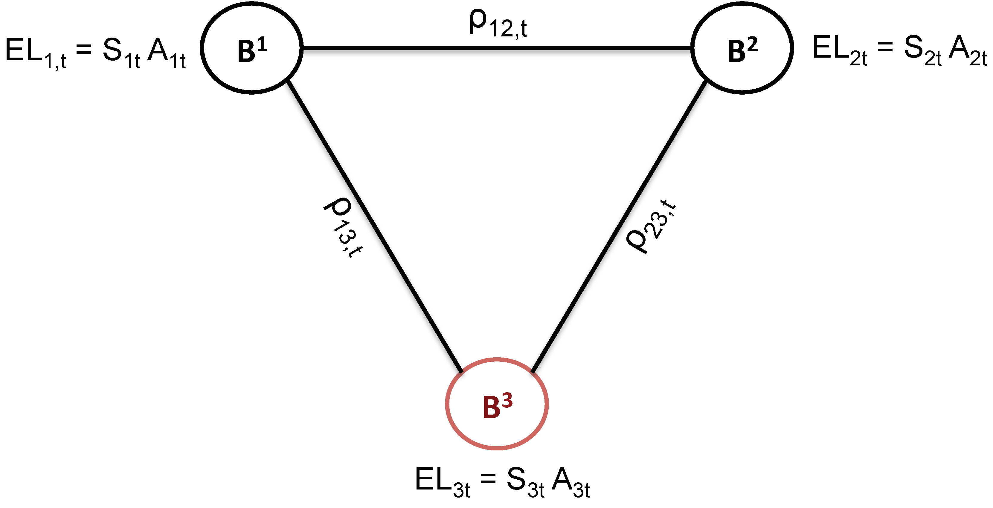
Consider a simplified system composed of three banks: $B^1$, $B^2$, and $B^3$, with the last one being in distress, as shown in Figure 1.

At any time, the three banks have an expected loss ($E{L}_n$), calculated as the product between their net assets ($A_n$) and their expected loss probability ($S_n$). In addition, they are all (directly) correlated with each other through partial correlation coefficients ${\rho }_{mn}$, which depend on the conditioning set.

To understand whether $B^1$ and $B^2$ will benefit more from the private intervention on $B^3$, rather than its liquidation or bail-in, we derive the time evolution of the total balance-sheets and spreads under the three scenarios. For simplicity, we consider three reference discrete times: $t_0$, $t_1$ and $t_2$. At time $t_1$, three events can occur: (a) $B^3$ is liquidated; (b) $B^3$ is recapitalized by $B^1$ and $B^2$; (c) $B^3$ is bailed in. At time $t_2$, the banking system will reach a new equilibrium, without (Scenario (a)) or with (Scenarios (b) and (c)) $B^3$.

2.2.1. Scenario (a): Liquidation

We assume that banks maintain their value in the considered time period: $A_{n,t_0}=A_{n,t_1}=A_{n,t_2}$. Moreover, we assume that the two safe banks, $B^1$ and $B^2$, maintain the same spread through time: $S_{\{1,2\},t_0}=S_{\{1,2\},t_1}=S_{\{1,2\},t_2}$. The distressed bank $B^3$ follows a different evolution: while its spread at time $t_0$ is $S_{3,t_0}$, in the following time period and in the liquidation scenario that $B^3$ defaults, so that $S_{t_1}^3=1$ (assuming $R{R}_3=0$). Finally, at time $t_2$, the distressed bank exits the system.

From a balance-sheet perspective, we assume that $B^3$ suffers severe losses at time $t_1$, which explain why that bank is considered to be in distress: at the same time, we suppose that the other two safe banks in the system have not been affected by losses. The rationale behind this setup is that we are not interested in understanding what may happen in case of an exogenous systemic crisis, but rather if systemic consequences might be triggered in case an endogenous distress event affects one bank. We then assume that at time $t_2$, the liquidation procedure is concluded, and thus, $B^3$ is not part of the system anymore: from a balance-sheet perspective, this means that its liabilities have been written down to cover losses. We can reasonably suppose that a portion k of such liabilities3 consists of cross-bank exposures. This implies that the other two banks in the system have lost a fraction, respectively equal to $f_1$ and $f_2$, of their balance-sheet. These fractions may be fixed by regulation authorities.

Partial correlation coefficients can be derived from the correlation matrix between the CDS spreads, along all the available time period. We suppose that the shock that $B^1$ and $B^2$ receive at time $t_1$, due to the liquidation of $B^3$, depends on the correlations between the two safe banks and the distressed bank $B^3$ observed at time $t_0$. At time $t_2$, after the liquidation of $B^3$, the banking system is composed by only two banks, $B^1$ and $B^2$, so that the correlation matrix becomes a $2\times 2$, rather than a $3\times 3$, matrix. A summary of the involved variables can be observed in

Table 1. Variables’ time-evolution, liquidation.

		${\mathit{t}}_0$	${\mathit{t}}_1$	${\mathit{t}}_2$
Assets	$B^1$	$A_1$	$A_1-f_1·k·[A_3-$ equity]	$A_1-f_1·k·[A_3-$ equity]
	$B^2$	$A_2$	$A_2-f_2·k·[A_3-$ equity]	$A_2-f_2·k·[A_3-$ equity]
	$B^3$	$A_3$	$A_3$	-
S	$B^1$	$S_1$	$S_1$	$S_1$
	$B^2$	$S_2$	$S_2$	$S_2$
	$B^3$	$S_{3,t_0}$	$S_{3,t_1}=1$	-
Marg.Corr.	$B^1$	$R_{t_0}$ ($3\times 3$)	$R_{t_0}$ ($3\times 3$)	$R_{t_2}$ ($2\times 2$)
	$B^2$
	$B^3$
Part.Corr.	$B^1$	${\left[{\left(R_{t_0}\right)}^{-1}\right]}_{mn}={\rho }_{mn|S}$	${\left[{\left(R_{t_0}\right)}^{-1}\right]}_{mn}={\rho }_{mn|S}$	${\left[{\left(R_{t_2}\right)}^{-1}\right]}_{mn}={\rho }_{mn|S,t_2}^a$
	$B^2$
	$B^3$

Notes: Time evolution of the variables that determine the total spreads of the three banks in the system, under the hypothesis that Bank 3 defaults at time $t_1$ (Scenario (a), liquidation).

.

We can calculate the total spread of each bank, at each discrete point in time $t_j$, by jointly computing the variables in Table 1 according to Equation (13). The total spreads can be then aggregated over time according to Equation (14): the results consist of an overall total spread for each bank, $T{S}_{n,T}^a$, where “overall” indicates the aggregation of the total spread over time and a refers to the liquidation scenario.

2.2.2. Scenario (b): Private Intervention

When $B^1$ and $B^2$ decide to participate in a private intervention in order to recapitalize $B^3$, we assume a proportional capital injection, meaning that the amount that the two safe banks have to use is proportional to their relative size. More precisely, we assume that the distressed bank $B^3$ needs a net asset value equal to X in order to absorb all losses while still meeting minimum regulatory requirements. The other two banks in the system should inject, respectively, a fraction $X^1$ and $X^2$ of their net asset values, as follows:

$$\left\{\begin{array}{c}{X}^1=X\frac{A_1}{A_1+A_2},\hfill \\ X^2=X\frac{A_2}{A_1+A_2}.\hfill \end{array}\right.$$

(22)

Consistent with (22), at times $t_1$ and $t_2$, the values of $B^1$ and $B^2$ are reduced by amounts $X^1$ and $X^2$, while the value of $B^3$ is increased by amount X. As concerns the spreads, we suppose that, as in the liquidation scenario, $B^1$ and $B^2$ maintain their spread constant over time, and so does $B^3$ until time $t_1$. However, differently from what happens under the liquidation hypothesis, $B^3$ does not default so that, at time $t_2$, $S_{3,t_2}\ne 1$. After a bank has been recapitalized, its spread at time $t_2$ is very likely to be smaller than before, as it is reasonable to imagine that a highly capitalized bank has gained market confidence; since we prefer being conservative, we assume that the worst scenario applies, so that $S_{3,t_2}=S_{3,t_1}=S_{3,t_0}$.

Partial correlations can be derived as in the liquidation scenario, the only difference being that now, at time $t_2$, the correlation matrix is a $3\times 3$ matrix since $B^3$ remains part of the banking system through time. A summary of the involved variables is reported in

Table 2. Variables’ time-evolution, private intervention.

		${\mathit{t}}_0$	${\mathit{t}}_1$	${\mathit{t}}_2$
Assets	$B^1$	$A_1$	$A_1(1-\frac{X}{A_1+A_2})$	$A_1(1-\frac{X}{A_1+A_2})$
	$B^2$	$A_2$	$A_2(1-\frac{X}{A_1+A_2})$	$A_2(1-\frac{X}{A_1+A_2})$
	$B^3$	$A_3$	$A_3+X$	$A_3+X$
S	$B^1$	$S_1$	$S_1$	$S_1$
	$B^2$	$S_2$	$S_2$	$S_2$
	$B^3$	$S_{3,t_0}$	$S_{3,t_0}$	$S_{3,t_2}$
Marg. Corr.	$B^1$	$R_{t_0}$ ($3\times 3$)	$R_{t_0}$ ($3\times 3$)	$R_{t_0}$ ($3\times 3$)
	$B^2$
	$B^3$
Part. Corr.	$B^1$	${\left[{\left(R_{t_0}\right)}^{-1}\right]}_{mn}={\rho }_{mn|S}$	${\left[{\left(R_{t_0}\right)}^{-1}\right]}_{mn}={\rho }_{mn|S}$	${\left[{\left(R_{t_0}\right)}^{-1}\right]}_{mn}={\rho }_{mn|S}$
	$B^2$
	$B^3$

Notes: Time evolution of the variables used for estimating the total spreads of the three banks in the system, under the assumption that Bank 3 is recapitalized by the other two through a private intervention at time $t_1$ (Scenario (b), private intervention).

.

We can calculate the total spread of each bank, at each discrete point in time $t_j$, by jointly computing the variables in Table 2 according to Equation (13). As in the liquidation scenario, the total spreads can be finally aggregated over time according to Equation (14): the results consist of an overall total spread for each bank, $T{S}_{n,T}^b$, where “overall” indicates the aggregation of the total spread over time and b refers to the private intervention scenario. These outcomes can then be compared with $T{S}_{n,T}^a$.

2.2.3. Scenario (c): Bail-In

As described in the introductory section, the bail-in tool considers the writing down and/or conversion of some liabilities according to a hierarchy structure strictly determined by the regulatory authority. According to the current regulation, in case of a distress event, the first action should consist of writing down a portion of going-concern capital, mainly expressed in terms of Common Equity Tier 1 (CET 1), to absorb losses: in line with the guiding principles of the BRRD and the SRMR, this response guarantees that shareholders bear the first burden. Since distressed banks have not only to cover all losses, but also to meet minimum regulatory requirements in order to avoid sanctions or restrictions, the second possible action, if needed, would consist of converting additional going-concern (Additional Tier 1) or gone-concern (Tier 2) capital into CET 1: this could serve both the loss-absorbing and the recapitalization functions. In case both gone-concern and going-concern capital are not sufficient to cover all losses while still ensuring regulatory requirements are not breached, and in case any other private action is excluded, the bail-in tool can be adopted, if and only if the SRB decides it is necessary in the public interest. Under this hypothesis, the competent or the resolution authorities would prescribe the reduction or conversion of senior debt (that we will call bail-in-able liabilities) into equity, with the objective to absorb potentially residual losses, to recapitalize the institution and reinstate market confidence. The current regulation also establishes the pari passu principle, according to which the bail-in should guarantee the equal treatment of creditors while still following the statutory rank of claims that would apply under the relevant insolvency law. On the other hand, the resolution authority has also the power to exclude some liabilities from bail-in for financial stability reasons.

Given the pari passu constraint and the fact that the possible exclusion of some liabilities from the bail-in process is ex-ante unknown, we ignore this latter opportunity, and we divide the banks’ balance-sheet on the funding side into three categories: regulatory capital, bail-in-able liabilities, and covered liabilities. In addition, we will not consider the possible intervention of the Single Resolution Fund, for two main reasons: first of all, because the SRF has not been fully built yet;4 second, because the inclusion of the SRF intervention can imply the payment of ex-post contributions by the other banks in the system in order to replenish the SRF, thus creating further contagion effects that we are not able to model since we have no data on ex-ante and (consequently) ex-post contributions. We also remark that, according to the CRR, CRD, and the EBAGuidelines, the failing or likely-to-fail point can be reached if a bank infringes the requirements on its capital position, on its liquidity position, or any other requirements for continuing authorization. The capital position of a bank is determined by Pillar 1 and Pillar 2 requirements,5 with the former one consisting of (a) a minimum requirement on CET 1 equal to 4.5%RWA (Risk Weighted Assets), (b) a minimum requirement on Tier 1 (T1) equal to 6%RWA, and (c) a minimum requirement on total capital (equal to T1 + AT2 (Additional Tier 2)) equal to 8%RWA. Given the fact that banks can convert T1 and AT2 into CET 1 while keeping the same level of total capital constant, we will focus only on the 8%RWA requirement on total capital.

Under the above-mentioned assumptions, we thus suppose that the liability side of banks’ balance-sheet is stressed by severe losses: the bail-in tool starts via the conversion of capital instruments into CET 1. If this is not enough to guarantee that all losses have been absorbed by banks without breaching the minimum requirements, we proceed with the conversion of bail-in-able liabilities, in the amount strictly necessary to meet the conditions on loss-absorbency and capital requirements. As previously underlined, beside market-driven contagion (through CDS price dynamics), the bail-in tool introduces a form of balance-sheet-driven contagion: a portion k of the bailed-in liabilities, in fact, consists of cross-bank exposures.6 This means that each bank j in the system that is a creditor of the bailed-in bank i would loose a portion $f_j$ of the fraction k of the bailed-in resources of bank i. The balance-sheet-structure of the safe and bailed-in banks are specified in

Table 3. Variables’ time-evolution, bail-in.

		${\mathit{t}}_0$	${\mathit{t}}_1$	${\mathit{t}}_2$
Assets	$B^1$	$A_1$	$A_1-f_1·k·$ Bail-in${}_3$	$A_1-f_1·k·$ Bail-in${}_3$
	$B^2$	$A_2$	$A_2-f_2·k·$ Bail-in${}_3$	$A_2-f_2·k·$ Bail-in${}_3$
	$B^3$	$A_3$	$A_3-$ Bail-in${}_3$	$A_3-$ Bail-in${}_3$
S	$B^1$	$S_1$	$S_1$	$S_1$
	$B^2$	$S_2$	$S_2$	$S_2$
	$B^3$	$S_3$	$S_3$	$S_3$
Marg. Corr.	$B^1$	$R_{t_0}$ ($3\times 3$)	$R_{t_0}$ ($3\times 3$)	$R_{t_0}$ ($3\times 3$)
	$B^2$
	$B^3$
Part. Corr.	$B^1$	${\left[{\left(R_{t_0}\right)}^{-1}\right]}_{mn}={\rho }_{mn|S}$	${\left[{\left(R_{t_0}\right)}^{-1}\right]}_{mn}={\rho }_{mn|S}$	${\left[{\left(R_{t_0}\right)}^{-1}\right]}_{mn}={\rho }_{mn|S}$
	$B^2$
	$B^3$

Notes: Time evolution of the variables used for estimating the total spreads of the three banks in the system, under the assumption that Bank 3 is subject to resolution (conversion of bail-in-able liabilities) at time $t_1$ (Scenario (c), bail-in).

, where we indicate with $A^3$ the total balance-sheet of the distressed bank after it has been affected by losses.

We remark that, in this scenario, the total amount of assets (or liabilities) is not preserved over time, as a result of bailed-in instruments and cross-bank exposures. In particular, at time $t_0$, we obtain:

$$T{A}_{t_0}=\sum _{j=1}^{N-1}{A}_{j,t_0}+A_{i,t_0},$$

(23)

while, by aggregating the total balance-sheet of banks at time $t_1$, we can derive the following:

$$T{A}_{t_1}=\sum _{j=1}^{N-1}{A}_{j,t_1}+A_{i,t_1}=\sum _{j=1}^{N-1}[A_{j,t_0}-f_j·k·Bail-in]=T{A}_{t_0}-k·Bail-in.$$

(24)

This result is substantially different from what has been modeled in the private intervention scenario: in this latter case, in fact, we model the precautionary recapitalization of the distressed bank, thus preventing (a) capital from shrinking and (b) bail-in from being triggered. As a consequence, the total balance-sheet of the distressed bank is not affected, and cross-bank exposures remain untouched, thus preventing also the balance-sheet of the other banks in the system from being reduced.

3. Application

3.1. The Banks’ Perspective

In this subsection, the objective is to understand which scenario minimizes each bank’s potential losses in case one bank in the system is under distress. We thus compare the total expected losses under two alternatives: (a) liquidation and (b) private intervention. We exclude the bail-in option in this part as, under Scenario (c), the troubled bank would keep being part of the banking system: by assuming that, in a system of only three banks, the contagion component deriving from cross-bank exposures is negligible, the bail-in scenario can be assimilated, from a single bank’s perspective, to Scenario (b).

The total expected losses of the three banks, aggregated over the entire time horizon and referring to the Scenarios (a) and (b) described above, can be summarized as follows:

$$\left\{\begin{array}{c}T{S}_{n\ne 3,T}^a=1-(1-T{S}_{n,t_0}^a)·(1-T{S}_{n,t_1}^a)·(1-T{S}_{n,t_2}^a),\hfill \\ T{S}_{3,T}^a=1,\hfill \\ T{S}_{n,T}^b=1-(1-T{S}_{n,t_0}^b)·(1-T{S}_{n,t_1}^b)·(1-T{S}_{n,t_2}^b).\hfill \end{array}\right.$$

(25)

To decide whether their participation in a private intervention to rescue $B_3$ would decrease their potential losses, the banks $B_1$ and $B_2$ should evaluate the difference between $T{S}_T^a$ and $T{S}_T^b$. If $T{S}_{n,T}^a-T{S}_{n,T}^b>0$, a capital injection towards $B_3$ would decrease their expected losses with respect to the liquidation scenario. Conversely, if $T{S}_{n,T}^a-T{S}_{n,T}^b<0$, the liquidation of $B_3$ would decrease their expected losses. The direct consequence is that each bank can decide whether to join a private recapitalization plan or not, according to which one of the two scenarios minimize its potential losses.

To better understand the determinants of the choice, we set up an experimental setup, as follows.

We assume that, among the three banks in the system, two banks are much larger than the third one, their sizes being $A_1=40$, $A_2=20$, and $A_3=4$ (billion Euros). To account for the largest range of variability, we randomly sample the partial correlation coefficients between the three banks from a continuous distribution, which allows us to include all the possible correlation values between zero and one, while also ensuring that all the possible combinations between the three coefficients can be explored. Without loss of generality, we select the Gaussian distribution ${\rho }_{mn}\sim \mathcal{N}({\mu }_{{\rho }_{mn}},{\sigma }_{{\rho }_{mn}}^2)$, centered in ${\mu }_{{\rho }_{12}}={\mu }_{{\rho }_{13}}={\mu }_{{\rho }_{23}}$ and with unit variances. Similarly, and for the same reasons explained before, we sample the CDS spreads of $B_1$ and $B_2$ from a Gaussian distribution, $S_n\sim \mathcal{N}({\mu }_{S_n},{\sigma }_{S_n}^2)$, with unit variances, but centered in four alternative mean values for the two safe banks: ${\mu }_{S_1},{\mu }_{S_2}=0.01,0.03,0.05,0.07$. While the CDS spreads of $B_1$ and $B_2$ remain constant over time, the CDS spreads of $B_3$ change, as follows:

$$\left\{\begin{array}{c}{S}_{3,t_j}\sim \mathcal{N}({\mu }_{S_{3,t_j}},{\sigma }_{S_3}^2),\hfill \\ {\mu }_{S_{3,\{t_0,t_1\}}}=0.10,\hfill \\ {\mu }_{S_{3,t_2}}\sim \mathcal{U}\left([0,0.10]\right),\hfill \end{array}\right.$$

(26)

with a unit variance. We remind that, under the liquidation scenario, $B_3$ disappears from the system at time $t_2$, meaning that, in this case, the last equation in (26) does not apply.

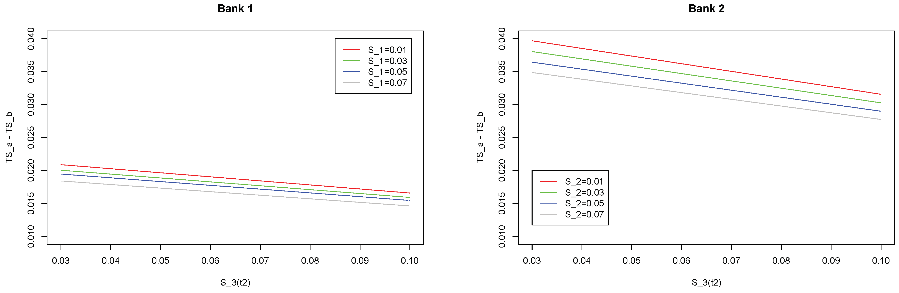
In each simulation run (10,000 simulations for each bank), we have thus sampled, from the previously-specified distributions and for each bank, two values for the two partial correlation coefficients and one value for the CDS spread, resulting in 10,000 simulated total spreads for each bank. The mean values of these differences, $T{S}_{n,T}^a-T{S}_{n,T}^b$, have been computed, and the corresponding results are shown in Figure 2. Our results, that we do not report due to the lack of space, show that the simulations’ results converge well before 10,000 simulations.

The results plotted in Figure 2 can be summarized as follows. First, in case of positive correlations, the private intervention scenario always minimizes the potential losses of the two safe banks. Second, the comparison between the two graphs shows that such an effect is stronger for the smaller bank $B^2$. Third, both graphs represent four lines according to four different values of the distributions’ average ${\mu }_{S_{1,2}}$, thus revealing that the safer a bank is, the greater the reduction in its potential losses when it joins a private intervention.

The previous simulations have been obtained with a fixed mean correlation value ${\mu }_{{\rho }_{mn}}$. However, this assumption can be too simplistic, especially in the liquidation scenario: as revealed by extensive literature, in fact, when a bank is failing or when the banking system is facing a crisis period, correlations between financial institutions increase in number and strength. To analyze this more realistic scenario, we have uniformly sampled also the distribution parameter ${\mu }_{{\rho }_{mn}}$, as follows:

$$\left\{\begin{array}{c}{\rho }_{mn}\sim \mathcal{N}({\mu }_{{\rho }_{mn}},{\sigma }_{{\rho }_{mn}}^2),\hfill \\ {\mu }_{{\rho }_{mn}}\sim \mathcal{U}\left([-1,1]\right),\hfill \end{array}\right.$$

(27)

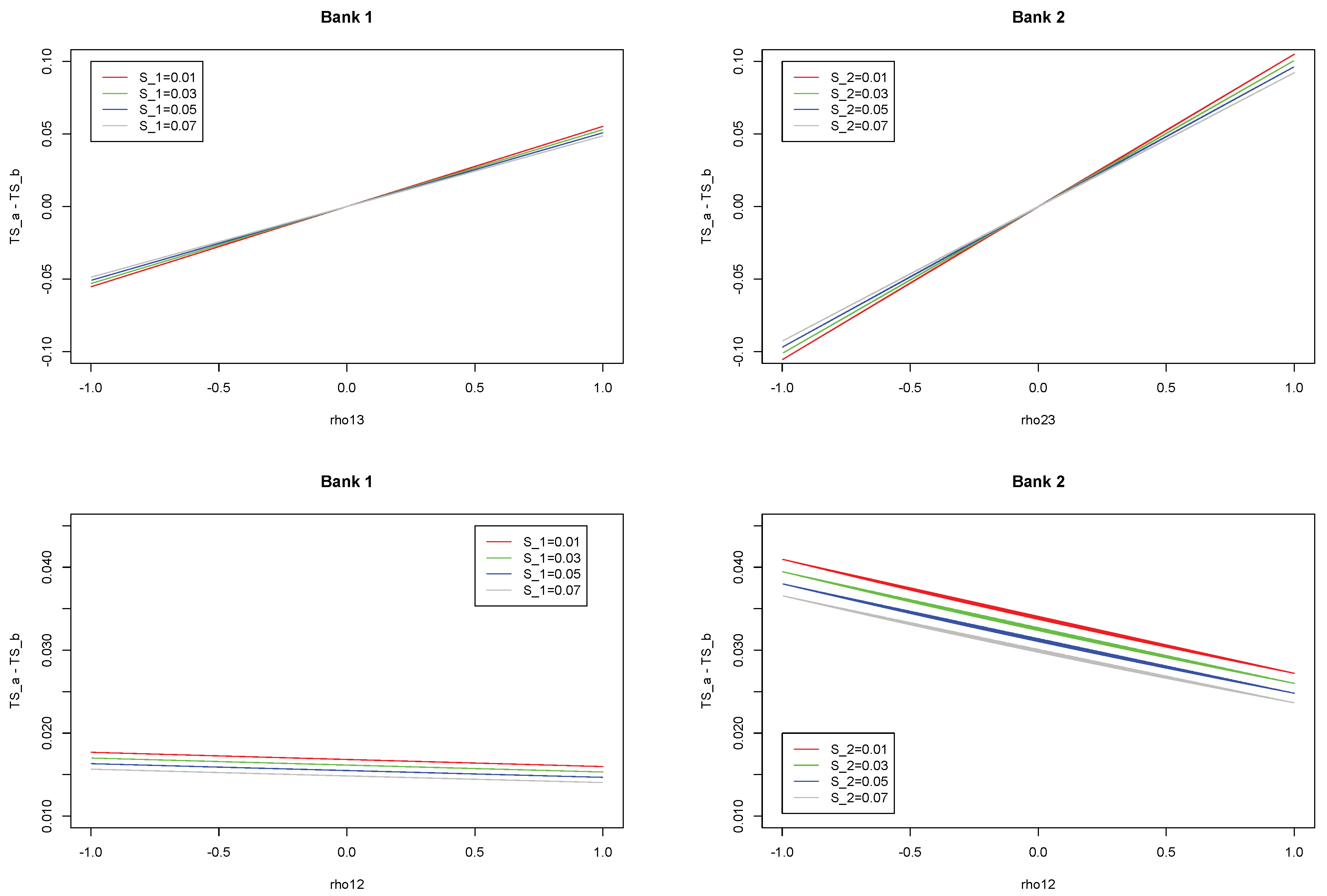
The resulting differences in $TS$, considered as functions of the sampled correlations and of the spreads of the safe banks (with ${\mu }_{S_{3,t_2}}=0.10$), are shown in Figure 3.

Figure 3 represents the decrease in the banks’ potential losses in case they recapitalize $B_3$ (private intervention scenario), as a function of the correlations between $B_1$ and $B_3$ (top-left), between $B_2$ and $B_3$ (top-right), and between the two safe banks $B_1$ and $B_2$ (bottom-left referring to $B_1$, bottom-right referring to $B_2$). The two top graphs show that the smaller the safe bank is, the stronger the dependence of expected losses on correlations. Second, in the case of positive correlations with $B^3$, the recapitalization scenario minimizes the potential losses; such a benefit is even stronger for smaller and safer banks. In case of negative correlations, the results are opposite: the liquidation scenario minimizes the potential losses, and the strength of such a result increases with the dimension of the safe bank.

The two bottom graphs show the impact of the correlation between the two safe banks $B^1$ and $B^2$ on the potential losses. The graph reveals that this impact is negligible for large banks (such as $B_1$), while it can be significant, even if low, for small banks: the weaker the correlation between $B_1$ and $B_2$, the bigger the loss reduction in the case of the private intervention scenario.

To summarize, by jointly reading Figure 2 and Figure 3, the results show that $B^1$ and $B^2$ overall reduce their potential losses in case they join a private intervention with respect to the liquidation scenario: this is not only true in the case of negative partial correlations between the safe banks. In addition, the reduction in their potential losses in case of a private intervention is (a) a decreasing function of the default probabilities of the safe banks, (b) a decreasing function of the dimension of the safe banks in the system, and (c) an increasing function of the correlation coefficients between the safe banks and the troubled institution.

3.2. The System Perspective

We now consider the Italian banking system. The rationale for this choice consists of the fact that Italian banks, even if strongly impacted by the global financial crisis and the subsequent European debt crisis, had not been subject to heavy public bail-out interventions before the BRRD came into place. On the other hand, a number of Italian banks have been found to be greatly undermined and considered as failing or likely to fail in the recent time period.

Our analysis is focused on the seven banks for which CDS data are available and reliable (source: Markit): Banca Popolare di Milano (BPM), Banco Popolare (BAPO), Intesa San Paolo (ISP), Mediobanca (MB), Monte dei Paschi di Siena (MPS), Unicredit (UCG), Unione Banche Italiane (UBI). We have considered daily frequencies for the period January–September 2016, since January 2016 corresponds to the concrete entry into play of the bail-in regulation. The summary statistics of CDS spreads are reported in

Table 4. CDS spreads.

Bank	$\mathit{\mu }$ (%)	Max (%)	Min (%)	$\mathit{\sigma }$ ($·{10}^{-2}$)
MPS	7.321	8.836	3.714	1.429
BPM	3.318	4.043	2.168	0.456
BAPO	3.771	4.871	2.608	0.484
MB	2.250	3.081	1.601	0.351
UCG	1.430	1.584	1.292	0.097
UBI	2.915	3.417	2.067	0.354
ISP	1.693	2.395	1.168	0.291

Notes: CDS spreads referring to seven Italian banks (MPS = Monte dei Paschi di Siena; BPM = Banca Popolare di Milano; BAPO = Banco Popolare; MB = Mediobanca; UCG = Unicredit; UBI = Unione Banche Italiane; ISP = Intesa San Paolo). The most troubled bank is MPS, with the highest mean value and volatility. The biggest banks (UCG and ISP) have the lowest and least volatile values.

. On the balance-sheet side, we have computed the banks’ net asset values by using the book values referring to 31 of December 2015 (source: Bureau Van Diyk Orbis Bank Focus): they are reported in

Table 5. Net asset values.

Bank	Net Asset Value
MPS	9.58
BPM	4.44
BAPO	6.92
MB	8.08
UCG	48.00
UBI	7.63
ISP	41.06

Notes: Net asset values referring to eight Italian banks (expressed in billion Euros).

.

Table 4 and Table 5 show that Monte dei Paschi di Siena (MPS) has the highest CDS spreads and the highest volatility within our sample. On the contrary, the two largest Italian banks (Unicredit and Intesa San Paolo) have the lowest CDS spreads, meaning they can highly rely on market confidence. Since MPS has the highest CDS spreads (with reference to our sample only), we assume it is the distressed bank in our system: this hypothesis is also in line with the recent facts, as MPS has been exceptionally recapitalized through public money in 2017, after intense discussions on whether a private intervention, liquidation, or bail-in should be considered.

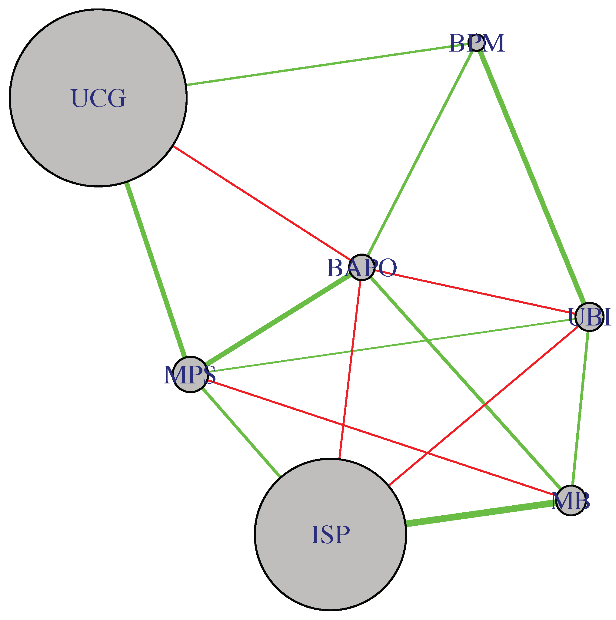
The computation of partial correlations relies on the time series of the expected losses of each bank, as derived in Equation (2). The resulting partial correlation networks are reported in Figure 4 and Figure 5: in the first figure, the size of each node is proportional to the average CDS spread of the corresponding bank, so to emphasize the importance of each financial institution in terms of its risk; in the second figure, the size of each node is proportional to the amount of total assets of the corresponding bank, so to emphasize the importance of each financial institution in terms of its relative dimension.

Figure 4 and Figure 5 reveal that the two largest banks are not strongly connected to each other, as well as they are not the most central institutions, both in terms of number of connections and correlation magnitudes. On the contrary, medium-sized banks, among which is the distressed bank MPS, are more interconnected.

Similarly to what has been described in the previous section, we can compute the total expected losses of each bank under alternative simulated values of CDS spreads and partial correlations, the difference being that now, we focus on all three scenarios and we adopt the system perspective. More precisely, we assume that:

$$\left\{\begin{array}{c}{S}_{n,t_j}\sim \mathcal{N}({\mu }_{S_{n,t_j}},{\sigma }_{S_n}^2),\hfill \\ {\mu }_{S_{MPS,t_2}}\sim \mathcal{U}\left([0,0.20]\right),\hfill \\ {\rho }_{mn}\sim \mathcal{N}({\mu }_{{\rho }_{mn}},{\sigma }_{{\rho }_{mn}}^2),\hfill \end{array}\right.$$

(28)

where the means ${\mu }_{S_{n,t_j}}$ for $n\ne MPS$ are fixed and based on the average CDS spreads. Similarly, ${\mu }_{S_{MPS,\{t_0,t_1\}}}$ are fixed and based on the CDS spreads in the first two periods, whereas in the last time period $t_2$, we extract the mean of the spread distribution referring to MPS from a uniform distribution. This choice allows the total spread of the other banks to depend on the increase or decrease of the MPS spreads in the case of private intervention or bail-in.

The previous equation reports the simulation setting for the market-based measures; however, we want to introduce a further degree of variability, which depends on balance-sheet items. Consistent with the methodology, in fact, we impose the following sampling distributions:

$$\left\{\begin{array}{c}{\mathrm{Losses}}_{n,t_0}\sim \mathcal{U}\left([0,{\mathrm{Bail}-\mathrm{in}}_{n,t_0}]\right),\hfill \\ {\mathrm{Equity}}_{n,t_0}\sim {\mathrm{Equity}}_{n,t_0-1}-{\mathrm{Losses}}_{n,t_0},\hfill \end{array}\right.$$

(29)

meaning that the equity structure of each bank at time $t_0$ is calculated through a shock in its initial values, due to potential losses that might affect the liabilities’ composition. The fractions $f_i$ (see Equation (24)) are proxied as the normalized values of partial correlations, while the parameter k is firstly chosen to be equal to 0.05 (meaning that 5% of the bailed-in liabilities consist of cross-bank exposures), but we will later let it vary between 0.01 and 0.50 for robustness purposes.

We remark that the distributional setting described so far does not exhaust all the possible contagion channels. We remark, in fact, that we model contagion as a cascade effect: this means that we start by shocking one node in the network, which corresponds to the bank identified as failing or likely-to-fail, and we then propagate the potential losses to the other nodes. As a consequence, this mechanism strictly depends on the propagation order we follow: to take this factor into account, we add a Monte Carlo simulation setting able to randomly select all the possible nodes’ permutations.

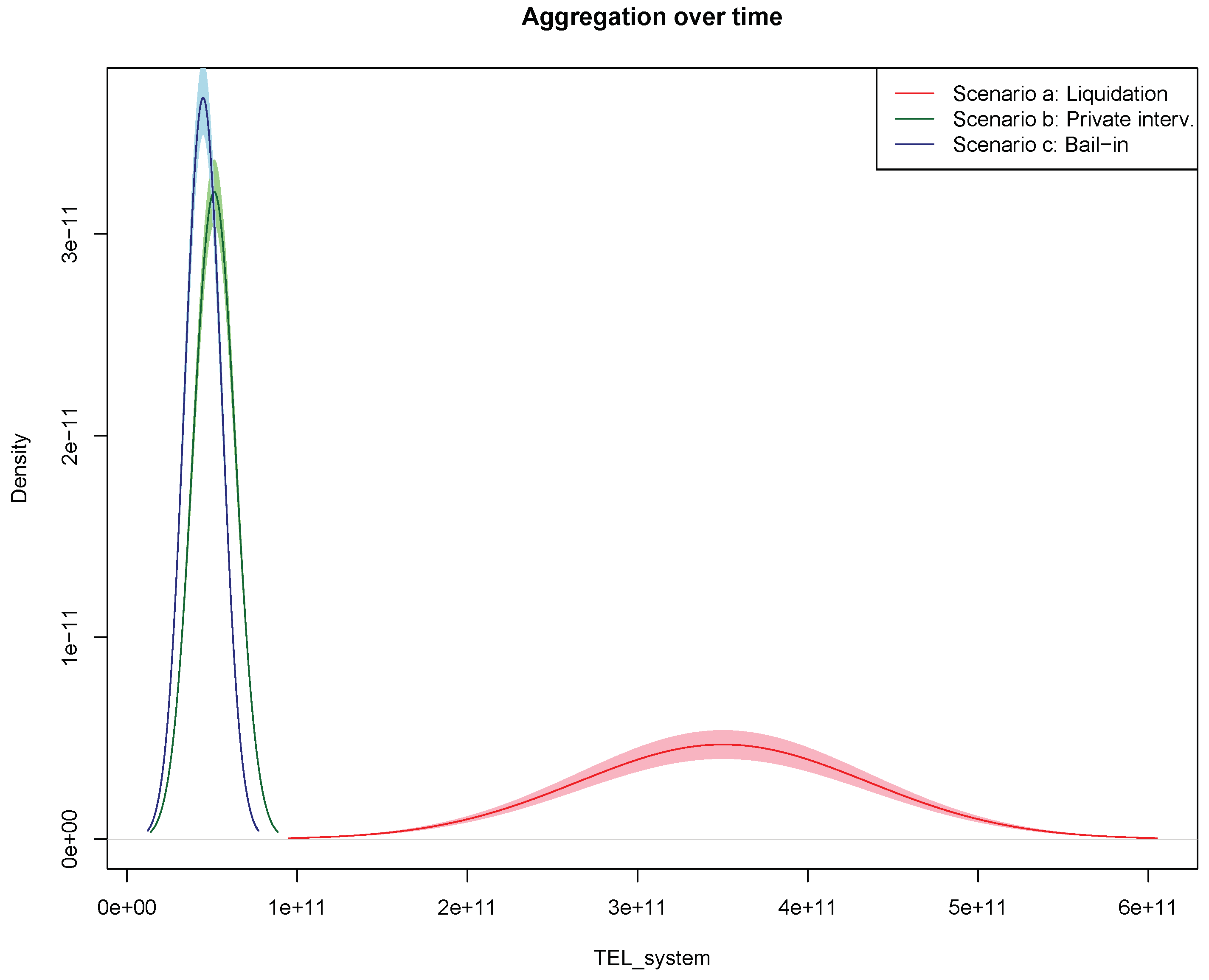
Finally, for each scenario and time period ($t_0$, $t_1$, $t_2$), we obtain a distribution of the potential losses for the banking system, built as a function of the different simulated values of the input variables and of the cascade permutations described above. The first results are shown in Figure 6: the top graph refers to $t_0$, the middle one to $t_1$, and the bottom chart to $t_2$; each graph shows the comparison between the distributions obtained in case of liquidation (red line), private intervention (green line), and bail-in (blue line).

The results in Figure 6 clearly show that the liquidation scenario strongly increases the expected losses of the system at time $t_1$ with respect to the private recapitalization or the bail-in resolution. The situation, however, appears almost reversed at time $t_2$: after the resolution decision, in fact, the liquidation hypothesis minimizes the potential losses for the banking system, since the exiting of the distressed institution from the network reduces the probability of adverse contagion effects across the system. The bail-in resolution tool, in addition, seems to restore the banking system better with respect to the private intervention scenario: this result is driven by the limited amount of cross-bank liabilities, as well as weaker post-resolution connections between the safe banks and the distressed bank (we remark that, by construction, the private recapitalization of the distressed institution, differently from resolution via bail-in, adds a further layer of connection among financial institutions).

Figure 7 aggregates the previous results over time and compares the overall potential losses under the three alternative scenarios.

The results in Figure 7 reveal that the potential losses for the banking system are minimized under the hypothesis of a private recapitalization or a bail-in resolution. As previously underlined, we remind that this result is also due to the relatively large size of MPS, which makes the shock produced in case of liquidation at time $t_1$ strongly negative in terms of loss propagation, thus prevailing over the beneficial effects liquidation would provide at time $t_2$. On the other hand, and also confirming our expectations, the bail-in resolution slightly reduces contagion effects with respect to the private intervention scenario.

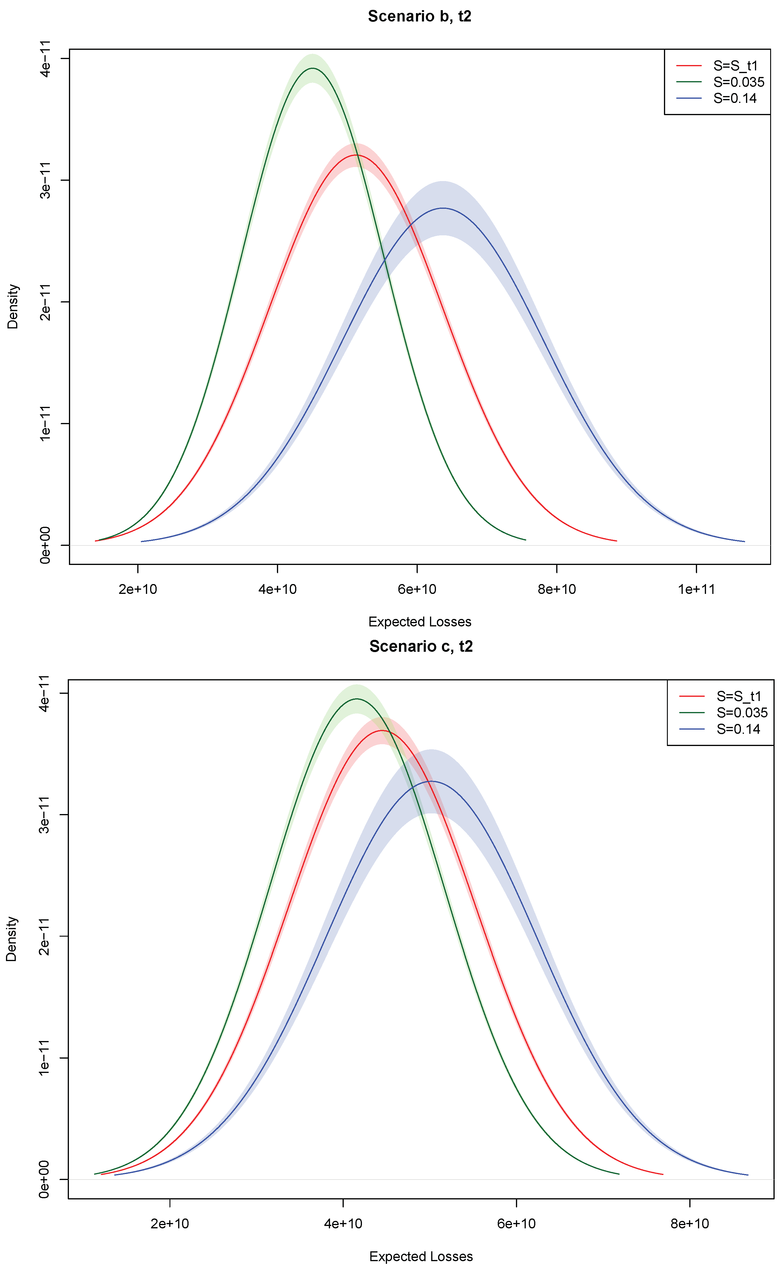
For robustness purposes, we also analyze how much the potential losses for the banking system would change according to different levels of idiosyncratic risk at time $t_2$: to this aim, we replicate the simulations by using different values of the CDS spreads of MPS at time $t_2$. These results are reported in Figure 8, and they refer, respectively, to the private intervention (top graph) and the bail-in (bottom graph) scenario.

In line with our expectation, Figure 8 reveals that, under both scenarios, the bigger the default probability of MPS at time $t_2$, the bigger the potential losses for the entire banking system at time $t_2$. In other words, when the distressed bank does not recover after the resolution decision by gaining market confidence (in our exercise modeled through an increase in its probability of default after the bail-in or private intervention decision), the potential losses of the entire system increase.

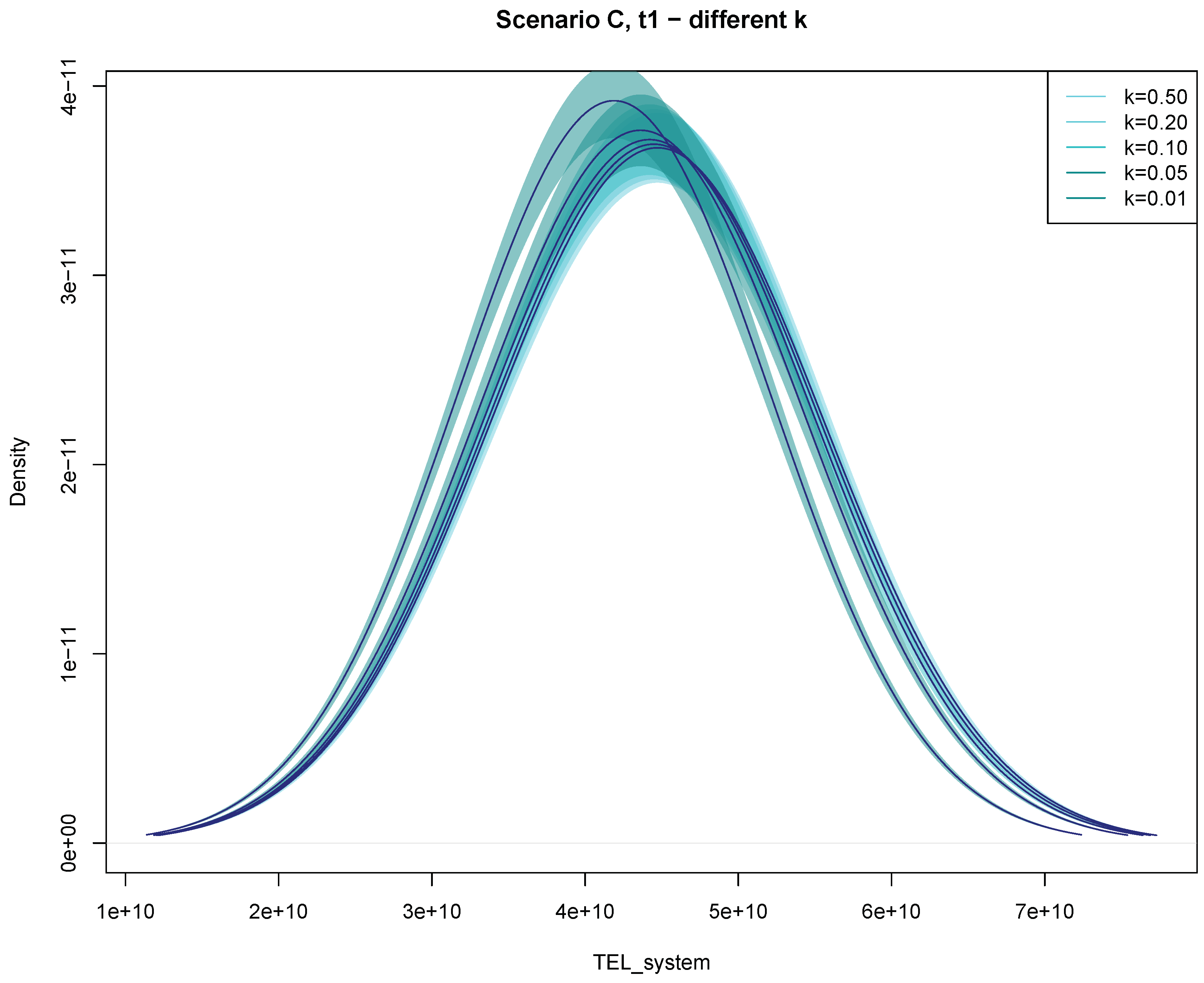
Finally, and again for robustness purposes, we can run a sensitivity analysis in order to understand to what extent the factor k affects the above-described results. Figure 9 reports the Monte Carlo simulated distributions of the potential system losses obtained under the bail-in scenario: each distribution corresponds to a different value of the parameter k, ranging from 1–50%.

Figure 9 shows that our results seem robust with respect to the choice of k: this robustness test also confirms that the bail-in tool, even if applied to all the bail-in-able liabilities of a distressed bank, would not produce substantial contagion effects triggered by cross-bank exposures.

To summarize, our empirical findings show that, from the system viewpoint, the best resolution decision on MPS would have been the resolution via bail-in, since it would have reduced the contagion effects via market-based or balance-sheet-based dynamics, thus limiting potential systemic risk effects. We remark, however, that our research considers the banking sector as a closed system and does not model the impact of distress events occurring in the banking sector in terms of macroeconomic consequences or indirect effects on tax payers (as shown for example in Beck et al. (2017)).

4. Conclusions and Policy Implications

We contribute to the financial econometric literature concerned with the measurement of systemic risk, by means of a novel correlation network model based on corporate default swap spreads, which improves their predictive accuracy. The model adds to the observed CDS spread a contagion component that is estimated through the observed correlation matrix between spreads, and it exploits the properties of partial correlation coefficients.

We also contribute to the central banking literature concerned with the resolution of financial institutions in light of the newly-adopted bail-in framework. We combine market-based measures, partial correlation networks and balance-sheet analyses to simulate the effects of different resolution plans, and to understand their consequences in terms of systemic risk. Our model derives the potential losses that could affect banks as a consequence of a financial institution identified as failing or likely to fail. Such losses are calculated under three alternative scenarios (liquidation, private intervention, and bail-in) and according to two perspectives (the bank’s and the system’s perspective). This allows the identification of the best resolution practice in terms of a loss minimization problem that, in our view, would reflect potential financial stability risks. As a consequence of a simulated distress event, our model is able to identify (a) which banks would minimize their potential losses in case they join a private intervention aiming at recapitalizing a failing or likely-to-fail bank and (b) which resolution plan would minimize the potential losses for the entire banking system.

From a single bank’s perspective, our empirical findings reveal that the recapitalization of a distressed financial institution via a private intervention always minimizes the potential losses for the other banks in the system, apart from the case of negative partial correlations. Furthermore, we found that the advantages of a private recapitalization are (a) a decreasing function of the default probabilities of the other (non-distressed) banks, (b) a decreasing function of the sizes of the other banks, and (c) an increasing function of the correlations between the safe banks and the distressed bank.

From the system perspective, a private intervention and a bail-in resolution would always reduce the potential losses of the banking sector with respect to the liquidation alternative. In addition, the bail-in resolution would slightly reduce the contagion effects with respect to the private recapitalization of the distressed banks. The outcomes of our analysis also show that in case the distressed bank does not recover after having been bailed-in or recapitalized (which is reflected by an increase in its default probability), the expected losses of the entire system increase: such increase is stronger in the private intervention scenario.

We believe that the methodology developed in this paper and the corresponding findings could be helpful guidelines in the context of a crisis event: for individual financial institutions, to decide whether to recapitalize privately a failing or likely-to-fail bank; and for resolution authorities, to have an additional tool to understand which resolution actions could be undertaken to preserve financial stability.

In terms of caveats, we are aware we have limited the scope of our analysis to a closed banking system, thus excluding the macroeconomic impacts (and loop-effects) of the above-described intervention scenarios. We recognize this assumption is strong and not too close to what would happen in a real crisis scenario: but we also believe that the joint modeling of financial and macroeconomic effects would require the involvement of too many factors and a long-term perspective, which would make the analysis either not feasible or not reliable in the long-run. We are also aware that we have performed a static, rather than a dynamic, analysis, although the latter may be difficult, in a network model context: in our view, a dynamic analysis would require an accurate estimation of after-crisis banks’ profitability, investors’ reliance, and managerial skills: this might be the objective of future research. A dynamical analysis may also consider whether multi-year CDS contracts modify the results.

We also remark that our contagion model is not based on distributional assumptions, and we recognize we could extend this paper in such a direction so to also derive confidence intervals for our results. Since a multivariate model for CDS spreads cannot be based on the Gaussian assumption, such improvement would require on to model interdependencies differently, for example by means of a Gaussian copula model or a skew copula model to account for asymmetric relationships.

References

- Abedifar, Pejman, Paolo Giudici, and Shatha Qamhieh Hashem. 2017. Heterogeneous market structures and systemic risk: Evidence from dual banking systems. Journal of Financial Stability 33: 96–119. [Google Scholar] [CrossRef]
- Acharya, Viral V., Lasse H. Pedersen, Thomas Philippon, and Matthew Richardson. 2010. Measuring Systemic Risk. Technical Report. New York: New York University. [Google Scholar]
- Acharya, Viral, Robert Engle, and Matthew Richardson. 2012. Capital shortfall: A new approach to ranking and regulating systemic risks. American Economic Review: Papers and Proceedings 102: 59–64. [Google Scholar] [CrossRef]
- Adrian, Tobias, and Markus K. Brunnermeier. 2016. “CoVaR. ” American Economic Review 106: 1705–41. [Google Scholar] [CrossRef]
- Ahelegbey, Daniel Felix, Monica Billio, and Roberto Casarin. 2015. Bayesian graphical models for structural vector autoregressive processes. Journal of Applied Econometrics 31: 357–86. [Google Scholar] [CrossRef]
- Avdjiev, Stefan, Paolo Giudici, and Alessandro Spelta. 2018. Measuring contagion risk in international banking. Journal of Financial Stability, 1–37. [Google Scholar] [CrossRef]
- Battiston, Stefano, Domenico Delli Gatti, Mauro Gallegati, Bruce Greenwald, and Joseph E. Stiglitz. 2012. Liasons dangereuses: Increasing connectivity risk sharing, and systemic risk. Journal of Economic Dynamics and Control 36: 1121–41. [Google Scholar] [CrossRef]
- Beck, Thorsten, Samuel Da-Rocha-Lopes, and André F. Silva. 2017. Sharing the Pain? Credit Supply and Real Effects of Bank Bail-Ins. Technical Report 12058. London: CEPR. [Google Scholar]
- Betz, Frank, Silviu Oprică, Tuomas A. Peltonen, and Peter Sarlin. 2014. Predicting distress in european banks. Journal of Banking and Finance 45: 225–41. [Google Scholar] [CrossRef]
- Billio, Monica, Mila Getmansky, Andrew W. Lo, and Loriana Pelizzon. 2012. Econometric measures of connectedness and systemic risk in the finance and insurance sectors. Journal of Financial Economics 104: 535–59. [Google Scholar] [CrossRef]
- Brownlees, Christian T., and Robert Engle. 2012. Volatility, Correlation and Tails for Systemic Risk Measurement. Technical Report. New York: New York University. [Google Scholar]
- Diebold, Francis X., and Kamil Yılmaz. 2014. On the network topology of variance decompositions: Measuring the connectedness of financial firms. Journal of Econometrics 182: 119–34. [Google Scholar] [CrossRef]
- Duffie, Darrell, and David Lando. 2001. Term structures of credit spreads with incomplete accounting information. Econometrica 69: 633–64. [Google Scholar] [CrossRef]
- Duprey, Thibaut, Benjamin Klaus, and Tuomas Peltonen. 2018. Dating systemic financial stress episodes in the eu countries. Journal of Financial Stability 32: 30–56. [Google Scholar] [CrossRef]
- Giudici, Paolo, and Alessandro Spelta. 2016. Graphical network models for international financial flows. Journal of Business and Economic Statistics 1: 128–38. [Google Scholar] [CrossRef]
- Giudici, Paolo, and Laura Parisi. 2018. Corisk: Credit risk contagion with correlation network models. Risks 6: 95. [Google Scholar] [CrossRef]
- Giudici, Paolo, Peter Sarlin, and Alessandro Spelta. 2017. The interconnected nature of banking systems: Direct and common exposures. Journal of Banking and Finance. [Google Scholar] [CrossRef]
- Hałaj, Grzegorz, Anne-Caroline Hüser, Christoffer Kok, Cristian Perales, and Anton Van der Kraaij. 2018. The Systemic Implications of Bail-In: A Multi-Layered Network Approach. Technical Report C. Frankfurt: European Central Bank. [Google Scholar]
- Hautsch, Nikolaus, Julia Schaumburg, and Melanie Schienle. 2015. Financial network systemic risk contributions. Review of Finance 19: 685–738. [Google Scholar] [CrossRef]
- Koopman, Siem Jan, André Lucas, and Bernd Schwaab. 2012. Dynamic factor models with macro, frailty, and industry effects for U.S. default counts: The credit crisis of 2008. Journal of Business and Economic Statistics 30: 521–32. [Google Scholar] [CrossRef]
- Lando, David, and Mads Stenbo Nielsen. 2010. Correlation in corporate defaults: Contagion or conditional independence. Journal of Financial Intermediation 19: 355–72. [Google Scholar] [CrossRef]
- Lorenz, Jan, Stefano Battiston, and Frank Schweitzer. 2009. Systemic risk in a unifying framework for cascading processes on networks. The European Physical Journal B—Condensed Matter and Complex Systems 71: 441–60. [Google Scholar] [CrossRef]
- Zhu, Haibin. 2006. An empirical comparison of credit spreads between the bond market and the credit default swap market. Journal of Financial Services Research 29: 211–35. [Google Scholar] [CrossRef]