Diversification and Systemic Risk: A Financial Network Perspective


Department of Finance, Accounting and Statistics, Vienna University of Economics and Business; 1020 Wien, Austria
*
Author to whom correspondence should be addressed.
†
These authors contributed equally to this work.
Risks 2018, 6(2), 54; https://doi.org/10.3390/risks6020054
Submission received: 9 April 2018
/
Revised: 2 May 2018
/
Accepted: 11 May 2018
/
Published: 15 May 2018
Abstract
:In this paper, we study the implications of diversification in the asset portfolios of banks for financial stability and systemic risk. Adding to the existing literature, we analyse this issue in a network model of the interbank market. We carry out a simulation study that determines the probability of a systemic crisis in the banking network as a function of both the level of diversification, and the connectivity and structure of the financial network. In contrast to earlier studies we find that diversification at the level of individual banks may be beneficial for financial stability even if it does lead to a higher asset return correlation across banks.
1. Introduction
The availability of modern risk-transfer tools enables banks to diversify away idiosyncratic risk concentrations in their portfolios. However, diversification at the level of individual banks might lead to more similar asset positions across banks and thus to a higher correlation of banks’ asset returns. This has sparked a debate on the merits of diversification in bank portfolios and on the impact of increasing asset return correlations on financial stability. Prior to the financial crisis, risk transfer between banks and diversification at the individual bank level was generally regarded as something positive. This view is for instance embodied in the following quotation from a 2002-speech of Alan Greenspan (then chairman of the Federal Reserve Board) to the council of foreign relations, see (Greenspan 2002).
Note that Greenspan explicitly entertains the idea that the default of any given financial institution may result in “cascading failures” of other banks via spillover effects in a network of direct credit relationships. In the presence of spillover effects, reducing idiosyncratic risk concentrations may thus be beneficial as it reduces the likelihood that individual banks default in the first place.[In the past year] I, particularly, have been focusing on innovations in the management of risk and some of the implications of those innovations for our global economic and financial system. The development of our paradigms for containing risk has emphasized dispersion of risk to those willing, and presumably able, to bear it. If risk is properly dispersed, shocks to the overall economic systems will be better absorbed and less likely to create cascading failures that could threaten financial stability.
After the financial crisis, diversification of bank portfolios and the potential increase in the correlation of banks’ asset returns were seen more critical. For instance, Wagner (2010) argued that, while diversification may indeed reduce the default probability of an individual bank, the ensuing rise in asset correlations increases the likelihood of a systemic banking crisis. (A systemic crisis is an event where a significant proportion of the financial institutions in the system defaults.) A similar conclusion was reached in (Beale et al. 2011). However, these two papers neglect potentially important network effects due to direct business links between financial institutions. Other contributions criticize a high level of correlation between banks’ asset portfolios on different grounds. For instance, Acharya and Yorulmazer (2007) argued that banks have an incentive to engage in herding behaviour to induce possible government bailouts.
Given these different views, the present paper is concerned with the impact of diversification at the level of individual banks (and hence a higher correlation of banks’ asset returns) on financial stability in a network model of financial institutions. The network represents direct financial links between banks such as a borrower–lender relationships. In this way, we include two important sources for a systemic banking crisis (correlation of asset returns and spillover effects via a network of direct financial linkages) in a single model. We use a simulation approach for our analysis: we randomly draw a financial network from a set of networks with given characteristics that reflect stylized facts observed in real-world interbank networks; subsequently, we generate a set of asset returns for the banks in the network. The use of randomly generated networks serves to robustify our analysis with respect to the details of the network topology. This is important since the exact structure of real-world financial networks is hard to observe due to a shortage of relevant data on financial linkages. We assume that a bank defaults if it is confronted with a sufficiently negative asset return (a so-called initial default). In that case, all its creditor banks suffer a loss. If this loss is sufficiently large, some of the creditor banks default as well, which then leads to further losses and possibly to a whole cascade of contagious defaults; this is the so-called default spillover effect.
In contrast to Wagner (2010) and Beale et al. (2011), we find in our setup that diversification at the level of individual banks is beneficial for financial stability, even though diversification leads to a higher level of asset-return correlation across banks. This difference is because, in our analysis, network-induced spillover effects are taken into account, whereas this source of systemic risk is ignored in the models of Wagner (2010) and Beale et al. (2011). Since direct financial linkages are an important feature of real-world banking systems, our results thus cast severe doubts on the policy conclusions reached in Wagner (2010) and Beale et al. (2011), lending instead some support to the pre-crisis view that diversification may foster financial stability, in line with Greenspan’s claim that “properly dispersed risk is less likely to produce cascading failures that threaten financial stability”.
Relation to the Literature on Systemic Risk
The present paper contributes to the growing literature on network models and default spillover effects. The vast majority of papers in this area use a two-step procedure. In the first step, they arrive at a financial network by direct observation, by estimation on the basis of disclosed financial statements, by asymptotic derivations for large and homogeneous networks (see Battiston et al. 2012) or by simulation methods (see Hurd et al. 2014; Hurd and Gleeson 2011). In the second step, it is assumed that an exogenously chosen set of banks (called initially defaulting banks) fails, and the effect on the system is analyzed. Models of this type are frequently used by regulators. Examples include Elsinger et al. (2006) (Austria), Upper and Worms (2004) (Germany), and Gai et al. (2011) (UK). Our setup differs from these contributions, since we generate the set of initial defaulting banks by an economically relevant mechanism and since we study the pros and cons of diversification. Our analysis is moreover related to the network models of Acemoglu et al. (2015) and Haldane and May (2011). In particular, the dichotomous behavior of default cascades observed in these papers (depending on the characteristics of the system, an exogenous return shock leads either to very few defaults or almost the entire network defaults) is observed in our setup as well. We briefly comment on the relation of our work to Acemoglu et al. (2015). The latter paper studies specific network structures (a fully connected network and a ring structure where every bank is connected to exactly one other firm) and it assumes independence between the exogenous return shocks experienced by the banks in the system. Given these assumptions Acemoglu et al. (2015) provide analytical results on the stability and the resilience of the financial system, and they establish the existence of a phase transition: if negative return shocks are sufficiently small, a more densely connected network enhances financial stability, for large return shocks on the other hand dense interconnections make the system more fragile. Our model allows for more realistic network structures and we consider correlation between return shocks, albeit at the loss of analytical results.
Influential early papers in the academic literature on contagion and financial networks include Allen and Gale (2000) and Eisenberg and Noe (2001); explicit bounds on spillover effects have been obtained in Glasserman and Young (2015). Network models are also becoming increasingly more popular in other areas of economics; see for example Braumolle et al. (2014) or Elliott et al. (2014), where the authors studied the joint effect of default spillovers and bank integration (see Section 2.1) by using a network model of crossholdings applied to European sovereign debt data.
An alternative strand in the systemic risk literature is concerned with the so-called systemic risk contribution of a financial firm, defined as the expected undercapitalization of the firm given that the financial system as a whole is under stress. A theoretical foundation for this approach was provided by Acharya et al. (2017); an empirical methodology to measure systemic risk contributions was developed by Brownlees and Engle (2017). The latter paper proposes the SRISK measure, defined as the expected capital shortfall of a financial institution given that the stock market as a whole experiences a severe decline. SRISK depends on the leverage ratio of the institution and on the conditional correlation of the institution’s stock returns to the market; Brownlees and Engle (2017) estimated this correlation via a DCC GARCH model.1 The literature on systemic risk contributions does not model the financial network explicitly; instead, it is based on the premise that the impact of financial linkages on the credit quality of a financial institution is priced correctly by the market so that it can be estimated from stock market data. As such, the SRISK methodology is complementary to the network models for systemic risk (such as our paper). SRISK provides very useful information for a regulator who needs to quantify the systemic risk contribution of financial firms using easily accessible data. On the other hand, the role played by the architecture of the financial system in shaping systemic risk is not addressed directly.
Further work on the empirical estimation of systemic risk includes the work of Billio et al. (2012) and Ali et al. (2016); an excellent survey on systemic risk measurement is given in Bisias et al. (2012).
2. Model and Methodology
2.1. The Model
2.1.1. The Financial Network
The network of interbank relationships is a central part of our model. Mathematically, this network can be described in terms of a directed graph consisting of N nodes indexed by . Each node represents a financial institution, while edges between them represent interbank credit exposures. More precisely, an edge from bank i to bank j means that bank j has a credit exposure towards bank i. This convention ensures that the direction of edges corresponds to the direction in which losses due to defaults spread through the network. The most obvious example of a credit exposure is an interbank loan made by bank j to bank i; alternatively, one might think of a counterparty-risk exposure incurred by bank j in a derivative transaction with bank i.
The graph2 is described by an adjacency matrix with elements satisfying:
In the sequel, we use the following notation to describe the balance sheet of the banks in the network. The total asset value of bank k is denoted by ; the nominal value of the loans made to other banks in the system is denoted by (short for interbank assets); the external assets such as loans to non-banks are denoted by ; and, finally, and represent the interbank liabilities and the external liabilities (e.g., customer deposits) of bank k, respectively, so that total liabilities are equal to . The equity of bank k is then given by . These quantities are illustrated in Table 1.
The following assumption permits us to create the financial network from a given adjacency matrix .
Assumption A1.
The financial network satisfies the following three conditions.
- (i)
- All loans in the system are of the same size, normalized to one.
- (ii)
- For every bank k in the network, the ratio (the ratio of equity over total assets) is equal to an exogenously given constant .
- (iii)
- For every bank k in the network, the ratio (the ratio of interbank assets to total assets) is equal to an exogenously given constant .3
Requirement (ii) can be viewed as a stylized version of the risk capital requirements imposed under the current Basel regulations. In the network literature (e.g., Elliott et al. (2014)), the parameter from (iii) is known as integration level of the network; a large means that the banking system is tightly integrated in the sense that banks do most of their business inside the banking network.
Roughly speaking, under Assumption 1, the financial network is created from in the following steps: first, Condition (i) is used to determine and for all banks . Using Condition (iii), we can then determine the overall asset value and hence also . Condition (ii) finally allows us to determine and hence also and . For details, we refer to Appendix A.
Our assumption slightly limits the model, since the level of bank leverage and interbank market integration is exogenously specified and homogenous across banks. We made these simplifying assumptions to focus primarily on the joint effect of diversification and network structure on financial stability. For a detailed analysis of the effect of interbank-market integration on systemic risk, see Elliott et al. (2014); the relevance of bank leverage for systemic risk and systemic risk contributions was discussed by Brownlees and Engle (2017).
2.1.2. Initial Defaults
In our setup, the return on the external assets of bank k, denoted , is random so that a sufficiently negative return shock can force a bank to default. We refer to this as an initial default and to the banks where this happens as initial defaulters, as a default due to a negative asset return happens at the start of a potential default cascade (see Section 2.2). Formally, an initial default occurs if the asset value after the return realization is lower than the liabilities of bank k, that is if
Since , an initial default thus occurs if . For banks with level of integration equal to (the typical case), this can be rewritten as
In other words, whether a bank is able to withstand a given return shock depends only on its integration in the interbank market and on the relative size of its capital buffer.
2.1.3. Diversification
We consider a particular model for asset returns where it is possibly for banks to diversify their external asset position; this allows us to study the impact of diversification on systemic risk. More precisely, we assume that there are N correlated investment opportunities for banks; investment opportunity (project) i has a return of the form
where and , are independent, -distributed random variables and where . Equation (3) implies that the return on different projects has a common factor which might be a natural assumption for the banking sector. The actual return of bank k is then modeled as a convex combination of and of the “market portfolio” , that is
For (no diversification), we have , whereas, for (perfect diversification), every bank holds the market portfolio given by . It is easily seen that, under Equation (4), the variance of (and hence the initial default probability) is decreasing in , essentially since the variance of the idiosyncratic part is reduced. In particular, we get that for the variance of is equal to , whereas for the variance of is equal to . Hence, can be viewed as a measure of the diversification of banks’ external asset portfolios4.
2.2. Spillover Effects
The idea underlying the spillover effect channel for systemic risk is simple. If a bank defaults in a financial network, it is unable to fulfill its obligations towards its creditors, which results in a reduction of the interbank assets of the creditor bank. If this loss is big enough, it may cause the creditor bank to default, so that default can become contagious and spread through the system. For simplicity, we assume zero recovery on defaulted interbank loans, such that one does not need to compute the value of recovery payments5.
For a given financial network, the mechanism that (potentially) generates a default cascade is described as follows:
- Perturb the external assets of each bank k by the return realization , that is let .
- If any of the banks defaults, propagate the shock to the asset side of its creditors. The new amount of interbank assets satisfies:
- If the total value of bank k’s assets falls below its liabilities, that is , bank k defaults.
- Repeat Steps 2 and 3 until there is no further default.
Note that, in our setup, the set of initially defaulting banks is generated by an economically relevant mechanism (Step 1 above). This is in contrasts to a large part of the literature on systemic risk in network models, where the initial defaulters are chosen in an ad hoc way.
2.3. The Network-Generation Process
To assess the relative importance and the joint effect of both channels for systemic risk, we conduct a two-layer Monte Carlo analysis. In the inner layer, we generate return realizations that follow Equation (4). This whole layer is embedded in the outer layer where 1000 random networks are created. The reason for using random graphs is the unobservable nature of real-world financial networks. As we are unable to observe the underlying financial network exactly6, we need to resort to a probabilistic framework. In this framework, only certain stylized facts about the system are specified and incorporated into the network generating process. In this way, each network can be seen as one realization of a random variable. This serves to robustify our analysis against misspecification of the underlying financial network while retaining the possibility to take qualitative properties of real-world financial networks into account.
To arrive at a proper network that describes mutual connections among financial institutions, we first need to sample an underlying adjacency matrix . For this, we use two different probabilistic models, namely a homogeneous Erdos–Renyi random graph and a inhomogeneous model that generates graphs with a core–periphery structure.
2.3.1. Homogeneous (Erdos–Renyi) Random Graphs
The Erdos–Renyi model is a simple reference model that is a popular benchmark for more sophisticated networks. In the Erdos–Renyi model, a random graph is generated such that the probability that there is an edge between any two nodes in the graph is a constant number ; put differently, every Erdos–Renyi random graph is parameterized only by two numbers—the number of nodes in the graph N and the probability that any two of them are connected. Moreover, connections are formed independent of each other, that is the elements , of are iid Bernoulli random variables. For , we get a complete directed graph in which every bank is connected to every other bank and vice versa, while, for , there are no links between the banks in the system.
2.3.2. Inhomogeneous (Core–Periphery) Random Graphs
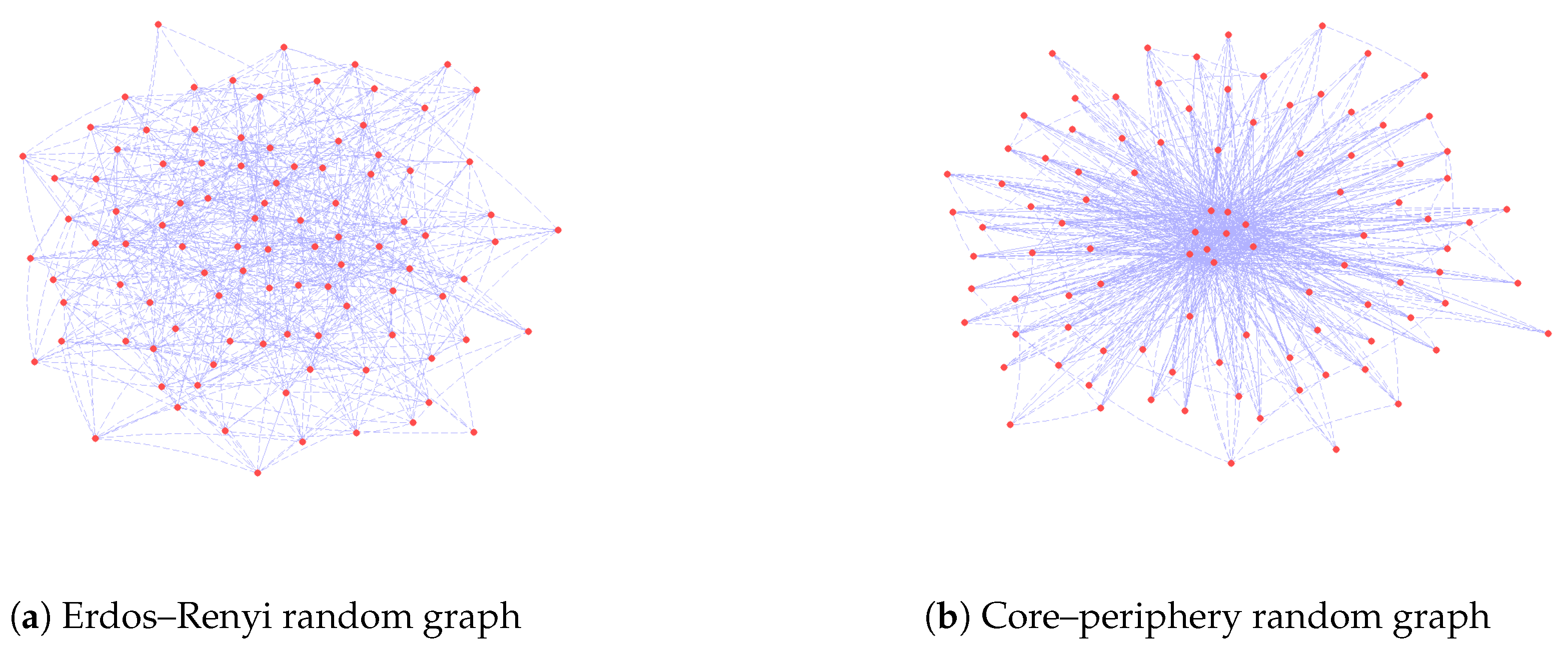
According to Soramäki et al. (2006), Bech and Atalay (2010), Iori et al. (2008) and others, a typical financial network exhibits a significant degree of so-called disassortativity, that is small banks tend to be connected to large ones and vice versa. An interpretation of this finding is that large banks act as intermediaries for smaller ones. To account for the observed disassortativity, we extend the Erdos–Renyi setting by making each bank belong either to a group called core with probability or to a group called periphery with a probability . The difference between these two groups of institutions lies in the probability of forming connections with other banks. A core bank has a large probability of establishing a connection both with other core banks and with other peripherals, while a connection between two peripherals is less likely. In this paper, we take the probability of a connection between two core banks equal to ; the probability of a connection between two peripheral banks is set to ; and the probability of a connection between a core bank and a peripheral in either direction is set to .7 Given the type of the banks in the system, connections are formed independent of each other. In this way, one ends up with an assortative network that we refer to as a core–periphery structure. The resulting network exhibits a star shape with few banks tightly connected in the center and the rest of the system on the periphery. In financial terms, core banks can be interpreted as large dealer banks that act as an intermediary for the other banks in the network. The difference between an Erdos–Renyi network and a core–periphery network is illustrated in Figure 1.
Note that, since a core bank has on average more connections than a peripheral bank, a higher value of leads to a higher density of the ensuing network. In particular, for , the whole network is formed by core banks so we actually get a very dense Erdos–Renyi setting (identical to the case where ), whereas, for , every bank is peripheral. Since peripherals are connected with probability , we get a sparse Erdos–Renyi setting (corresponding to ). Therefore, an intermediate level of corresponds to a network which lies between two homogeneous Erdos–Renyi extremes. In the Monte Carlo simulations, the probability of belonging to the core is varied between 0% and 20%.8
3. Results
We now present the results of a simulation study that illustrates the impact of the diversification and of the density or connectivity of the network on financial stability. We measure the density of a given network by the expected number of counterparties of a randomly chosen bank in the system.9 We call this quantity connectivity and denote it by C. In the Erdos–Renyi random graph, connectivity is given by ; in the case of a core–periphery network, connectivity is easily seen to be
The output variable in our analysis is the relative frequency of scenarios in the simulation in which a systemic crisis occurred. Here, a scenario is viewed as one realization of random network together with one realization of random returns, and a systemic crisis is defined as a scenario where more than 20% of all banks in the network are in default at the end of the default cascade. In the sequel, we call this relative frequency simply the probability of a systemic crisis. Note that the exact value of the threshold in the definition of a systemic crisis (20% or different) is irrelevant. In fact, for all but very small values of the connectivity parameter C, we observed a dichotomous behavior: in a given scenario, there are either very few defaults or the network is wiped out (almost) entirely. This dichotomous behavior was observed for both network types and for all values of and is consistent with findings from the literature (e.g., Acemoglu et al. 2015; Haldane and May 2011).
In Figure 2a,b, we plot the probability of a systemic crisis as a function of the diversification parameter for fixed values of the connectivity C, for both network types. We unambiguously find that an increase in the level of diversification lowers the probability of a systemic crisis. Note that this effect is higher for medium-to-high levels of connectivity. This permits us to conclude that the beneficial impact of diversification on financial stability is due to the incorporation of network effects. An intuitive explanation of this observation is as follows: in a financial network, a relatively small number of initial defaults is sufficient to cause a systemic crisis via spillovers. Moreover, the probability of observing at least a small number of initial defaults is higher if banks do not diversify: first, a more diversified asset portfolio has a lower variance, reducing the initial default probability; and second, the probability of observing at least one initial default decreases with increasing correlation of asset returns across banks, an effect that is well known from the literature on portfolio credit risk such as Frey and McNeil (2003).
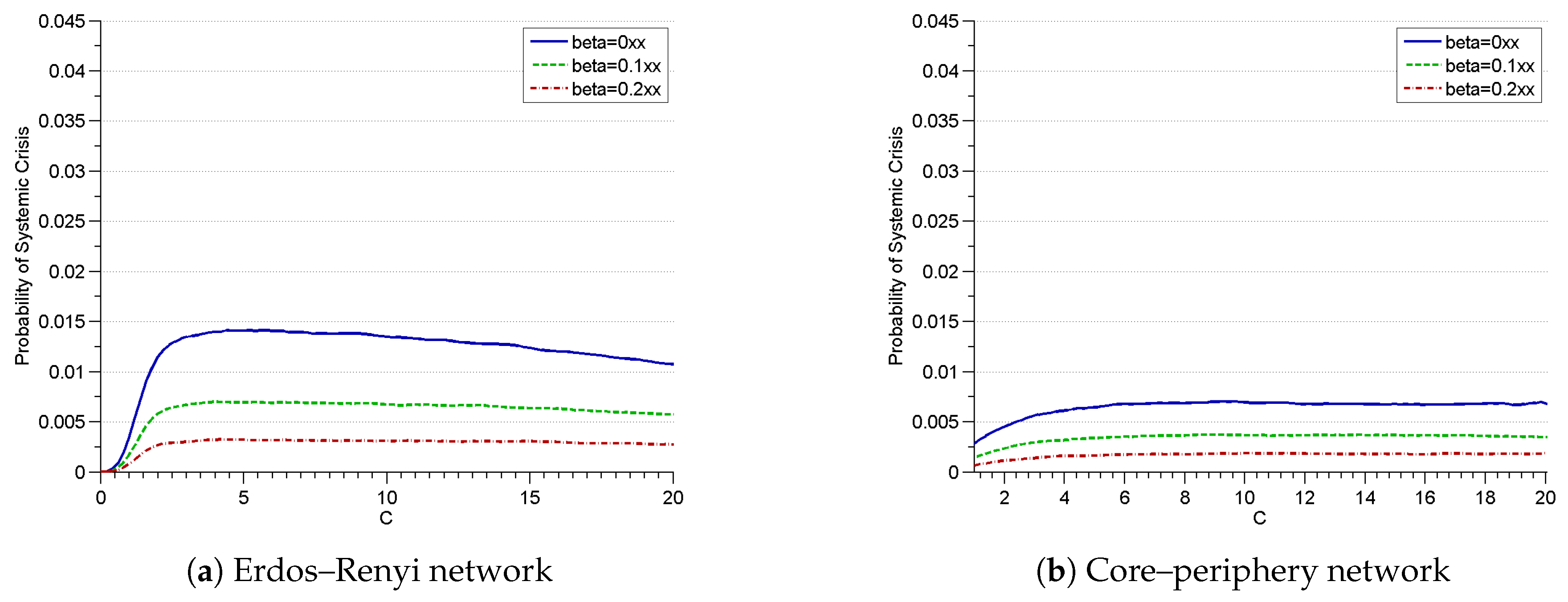
In Figure 3a,b, we plot the probability of a systemic crisis as a function of the connectivity C, keeping the diversification parameter fixed. We find that the probability of a crisis exhibits a hump-shaped behavior with an intermediate level of connectivity being the most dangerous. This is in line with other studies (see, for instance, Hurd et al. (2014)).
We have considered several variants of the model, leading to qualitatively similar results. Among others, we considered the case where the equity capital ratio of core institutions is higher than the equity ratio of peripherals. We found that this modification significantly reduces the probability of a systemic crisis, which supports proposals to regulate systemically important institutions more tightly.
4. Conclusions
We have studied the impact of diversification at the individual-bank level on systemic risk in a network model of the interbank market. Our analysis used a simulation approach; both a simple homogeneous Erdos–Renyi network and a more realistic inhomogeneous core–periphery network were examined in the process. It turned out that, in the presence of network effects, diversification of banks’ external assets is usually beneficial for financial stability. This finding is in stark contrast to the results of Wagner (2010) and Beale et al. (2011). We conclude that, to judge the implications of diversification on the magnitude of systemic risk, one needs to take direct financial linkages into account. Moreover, the scientific foundation for the policy recommendations made by Wagner (2010) and Beale et al. (2011) might be weaker than is claimed by these authors. Our model suggests that financial regulation rewarding banks that hold well diversified credit portfolios may not only decrease their individual levels of risk, but also contribute to a higher systemic stability.
Author Contributions
“Conceptualization, Methodology, Formal Analysis and Writing R.F. and J.H.; Software, and Visualization J.H.; Writing—Review & Editing, Project Administration, Funding Acquisition, R.F.”
Funding
Financial support from the Austrian Science Fund FWF via the Vienna Graduate School in Finance VGSF is gratefully acknowledged.
Acknowledgments
We would like to thank the faculty and students of VGSF as well as Branko Urosevic and Giovanni Calice for useful feedback. Our thanks also go to the participants of Systemic Risk workshops at the Isaac Newton Institute, Cambridge; participants of the 8th International Risk Forum in Paris; participants of the SYRTO conference in Amsterdam; and participants of the Conference for Young Economists in Belgrade.
Conflicts of Interest
The authors declare no conflict of interest.
Appendix A. The Financial Network
In this section, we refine Assumption 1 and we explain in detail how this assumption can be used to determine a financial network. First note that Condition (i) of Assumption 1 implies that bank k’s interbank assets are given by the number of its debtors and the interbank liabilities are equal to the number of its creditors, that is
where are elements of the adjacency matrix defined in Equation (1). Next, we take Assumption 1 (iii) on the level of integration . Loosely speaking, we assume that the level of integration is equal to an exogenously given constant or, equivalently, that . However, this is not always consistent with the requirement that the external liabilities are nonnegative. In fact, the requirement that gives that
and hence the inequality . Therefore, the total asset value of bank k is given by10.
For typical parameterizations of the model, is significantly larger than . In that case, if , the first term from (A2) is binding so that in fact . If is much larger than , the second inequality is binding and ensures that the total balance sheet size is not lower than the sum of interbank liabilities and equity. Such cases are extremely rare in our model and we only specify the complete rule here for the sake of completeness. For a given total asset value of bank k, the capital buffer is determined by Assumption 1 (ii). The external assets are finally given by the difference of total assets and interbank assets; similarly, the external liabilities are given by the difference between total liabilities and the sum of interbank liabilities and capital buffer . This gives, as ,
To summarize, Assumption 1 permits us to create a balance sheet structure from a given adjacency matrix along the following steps:
References
- Acemoglu, Daron, Asuman Ozdaglar, and Alireza Tahbaz-Salehi. 2015. Systemic risk and stability in financial networks. American Economic Review 105: 564–608. [Google Scholar] [CrossRef]
- Acharya, Viral V., Lasse H. Pedersen, Thomas Philippon, and Matthew Richardson. 2017. Measuring systemic risk. Review of Financial Studies 30: 2–47. [Google Scholar] [CrossRef]
- Acharya, Viral V., and Tanju Yorulmazer. 2007. Too many to fail—An analysis of time-inconsistency in bank closure policies. Journal of Financial Intermediation 16: 1–31. [Google Scholar] [CrossRef]
- Ali, Robleh, Nick Vause, and Filip Zikes. 2016. Systemic Risk in Derivative Markets: A Pilot Study Using CDS Data. London: Bank of England. [Google Scholar]
- Allen, Franklin, and Douglas Gale. 2000. Financial contagion. The Journal of Political Economy 108: 1–33. [Google Scholar] [CrossRef]
- Battiston, Stefano, Domenico Delli Gatti, Mauro Gallegati, Bruce C. N. Greenwald, and Joseph E. Stiglitz. 2012. Credit default cascades: When does risk diversification increase stability? Journal of Financial Stability 8: 138–49. [Google Scholar] [CrossRef]
- Beale, Nicholas, David G. Rand, Heather Battey, Karen Croxson, Robert May, and Martin Nowak. 2011. Individual versus systemic risk and the Regulator’s Dilemma. Proceedings of the National Academy of Sciences of the USA 108: 12647–52. [Google Scholar] [CrossRef] [PubMed]
- Bech, Morten L., and Enghin Atalay. 2010. The topology of the federal funds market. Physica A: Statistical Mechanics and Its Application 389: 5223–46. [Google Scholar] [CrossRef]
- Billio, Monica, Mila Getmansky, Andrew W. Lo, and Loriana Pelizzon. 2015. Econometric measures of connectedness and systemic risk in the finance and insurance sectors. Journal of Financial Economics 104: 535–59. [Google Scholar] [CrossRef]
- Bisias, Dimitrios, Mark Flood, Andrew W. Lo, and Stavros Valavanis. 2012. A survey of systemic risk analysis. Annual Review of Financial Economics 4: 255–96. [Google Scholar] [CrossRef]
- Braumolle, Yann, Rachel Kranton, and Martin D’Amours. 2014. Strategic interaction and networks. American Economic Review 104: 898–930. [Google Scholar] [CrossRef]
- Brownlees, Christian, and Robert Engle. 2017. SRISK: A conditional shortfall measure of systemic risk. Review of Financial Studies 30: 48–79. [Google Scholar] [CrossRef]
- Eisenberg, Larry, and Thomas H. Noe. 2001. Systemic risk in financial systems. Management Science 47: 236–49. [Google Scholar] [CrossRef]
- Elliott, Matthew, Benjamin Golub, and Matthew O. Jackson. 2014. Financial networks and contagion. American Economic Review 104: 3115–53. [Google Scholar] [CrossRef]
- Elsinger, Helmut, Alfred Lehar, and Martin Summer. 2006. Using market information for banking system risk assessment. International Journal of Central Banking 2: 137–65. [Google Scholar] [CrossRef] [Green Version]
- Frey, Rüdiger, and Alexander J. McNeil. 2003. Dependent defaults in models of portfolio credit risk. The Journal of Risk 6: 59–92. [Google Scholar] [CrossRef]
- Gai, Prasanna, Andrew Haldane, and Sujit Kapadia. 2011. Complexity, concentration and contagion. Journal of Monetary Economics 58: 453–70. [Google Scholar] [CrossRef]
- Glasserman, Paul, and H. Peyton Young. 2015. How likely is contagion in financial networks? Journal of Banking and Finance 50: 383–99. [Google Scholar] [CrossRef]
- Greenspan, Alan. 2002. Speech before the Council of Foreign Relations. Washington: International Financial Risk Management. [Google Scholar]
- Haldane, Andrew, and Robert M. May. 2011. Systemic Risk in Banking Ecosystems. Nature 469: 351–55. [Google Scholar] [CrossRef] [PubMed]
- Hurd, Tom, Davide Cellai, Huibin Cheng, Sergey Melnik, and Quentin Shao. 2014. Illiquidity and insolvency: A double cascade model of financial crises. arXiv, arXiv:1310.6873. [Google Scholar]
- Hurd, Tom R., and James P. Gleeson. 2011. A framework for analyzing contagion in banking networks. arXiv, arXiv:1110.4312. [Google Scholar]
- Iori, Giulia, Giulia De Masi, Ovidiu Vasile Precup, Giampaolo Gabbi, and Guido Caldarelli. 2008. A network analysis of the italian overnight money market. Journal of Economic Dynamics and Control 32: 259–78. [Google Scholar] [CrossRef]
- Soramäki, Kimmo, Morten L. Bech, Jeffrey Arnold, Robert J. Glass, and Walter E. Beyeler. 2006. The Topology of Interbank Payment Flows. Staff Reports. New York: Federal Research Bank of New York, p. 243. [Google Scholar]
- Upper, Christian, and Andreas Worms. 2004. Estimating bilateral exposures in the german interbank market: Is there a danger of contagion? European Economic Review 48: 827–49. [Google Scholar] [CrossRef]
- Wagner, Wolf. 2010. Diversification at financial institutions and systemic crises. Journal of Financial Intermediation 19: 373–86. [Google Scholar] [CrossRef]
| 1 | For empirical details and real time estimates of the SRISK measure, we refer to the work of the VLAB run by Robert Engle at NYU Stern School of Business, see https://vlab.stern.nyu.edu/. |
| 2 | Throughout the paper, we use the terms graph and network. When talking about a graph, we are concerned with the structure of financial linkages, whereas, when referring to a network, we mean not just connections themselves but also balance sheet quantities of individual banks. |
| 3 | This assumption needs to be refined slightly to avoid certain extreme cases where becomes negative; see Appendix A for details. |
| 4 | Note that we assume that the asset returns of banks are diversified from the outset; potential problems with securitization and credit risk transfer are not the focus of our paper. |
| 5 | Thanks to this assumption, there is no need for a settlement algorithm in the spirit of Eisenberg and Noe (2001). Assuming non-zero recovery rate on distressed loans would however not change the overall quantitative nature of our results. |
| 6 | There are just a few countries where regulators possess reasonably good data on the structure of the interbank market, for example Austria, Mexico, Germany or Brazil. |
| 7 | These parameter values are typical for the Austrian interbank market. |
| 8 | A regulator with access to real data could apply our approach to an actual interbank network. In that situation, one would use some centrality measure to classify a subset of important banks as hubs that form the core of the network. This immediately yields , and the other parameters are then easy to estimate. |
| 9 | In graph theoretic literature, this is known as the average graph degree. |
| 10 | In a special case where a bank has no connections at all, we assume that it puts a portion of its total assets into some riskless investment (such as government bonds) and 1- into risky external assets. We also assume that the size of the balance sheet is 1. We make this technical assumption to prevent banks from having their balance sheet size equal to zero. Note that this assumption has no effect on the analysis itself since a bank with no connections does not affect the rest of system. |
Figure 1.
One realization of a random graph for banks: (a) Erdos–Renyi network; and (b) core–periphery network.
Figure 1.
One realization of a random graph for banks: (a) Erdos–Renyi network; and (b) core–periphery network.

Figure 2.
Probability of a systemic crisis for both network structures on nodes as a function of diversification for particular levels of connectivity C. Bank equity ratio , integration and correlation of project returns (see Equation (3)) .
Figure 2.
Probability of a systemic crisis for both network structures on nodes as a function of diversification for particular levels of connectivity C. Bank equity ratio , integration and correlation of project returns (see Equation (3)) .
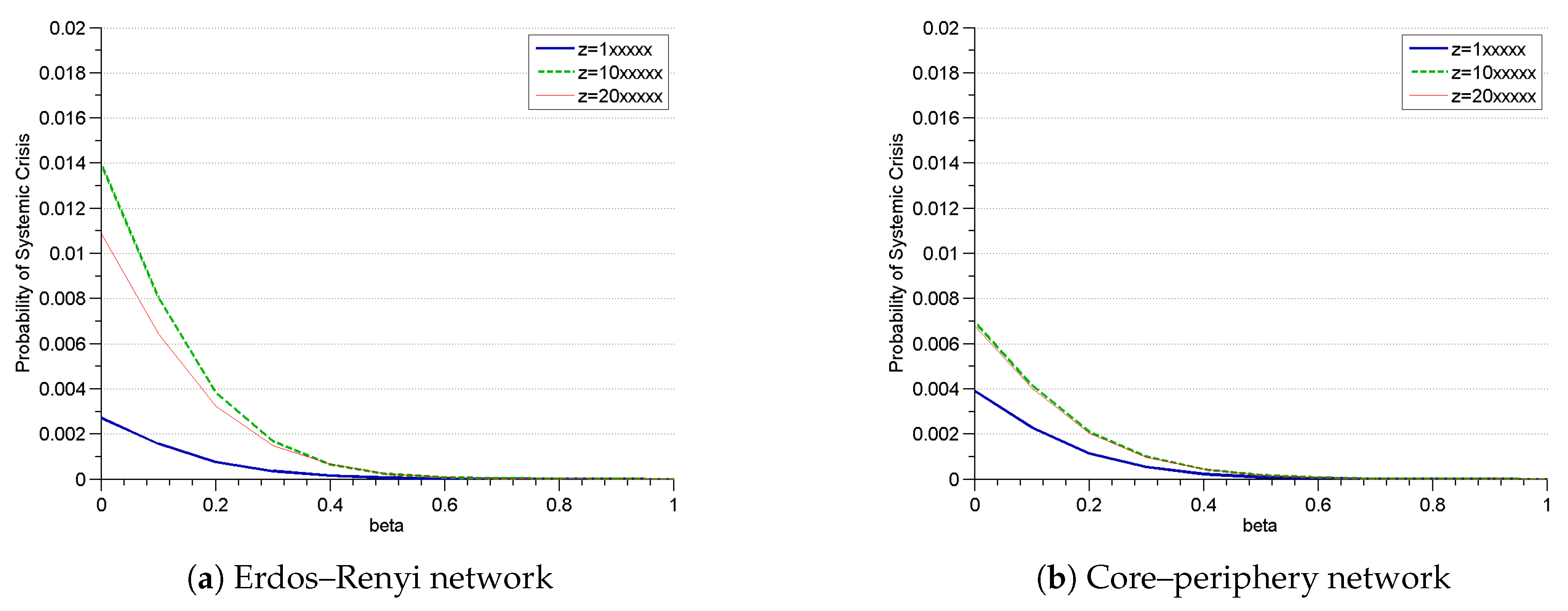
Figure 3.
Probability of a systemic crisis for both network structures on nodes as a function of connectivity C for particular levels of diversification . Bank equity ratio , integration and correlation of project returns (see (3)).
Figure 3.
Probability of a systemic crisis for both network structures on nodes as a function of connectivity C for particular levels of diversification . Bank equity ratio , integration and correlation of project returns (see (3)).

Table 1.
Balance sheet of bank k.
| Assets | Liabilities |
|---|---|
| interbank assets | interbank liabilities |
| external assets | external liabilities |
| equity | |
| total assets | total liabilities |
© 2018 by the authors. Licensee MDPI, Basel, Switzerland. This article is an open access article distributed under the terms and conditions of the Creative Commons Attribution (CC BY) license (http://creativecommons.org/licenses/by/4.0/).
Share and Cite
MDPI and ACS Style
Frey, R.; Hledik, J. Diversification and Systemic Risk: A Financial Network Perspective. Risks 2018, 6, 54. https://doi.org/10.3390/risks6020054
AMA Style
Frey R, Hledik J. Diversification and Systemic Risk: A Financial Network Perspective. Risks. 2018; 6(2):54. https://doi.org/10.3390/risks6020054
Chicago/Turabian StyleFrey, Rüdiger, and Juraj Hledik. 2018. "Diversification and Systemic Risk: A Financial Network Perspective" Risks 6, no. 2: 54. https://doi.org/10.3390/risks6020054
Note that from the first issue of 2016, this journal uses article numbers instead of page numbers. See further details here.