A General Framework for Portfolio Theory—Part I: Theory and Various Models


1
Institut für Mathematik, RWTH Aachen University, Templergraben 55, 52062 Aachen, Germany
2
Department of Mathematics, Western Michigan University, 1903 West Michigan Avenue, Kalamazoo, MI 49008, USA
*
Author to whom correspondence should be addressed.
Risks 2018, 6(2), 53; https://doi.org/10.3390/risks6020053
Submission received: 30 March 2018
/
Revised: 23 April 2018
/
Accepted: 1 May 2018
/
Published: 8 May 2018
(This article belongs to the Special Issue Computational Methods for Risk Management in Economics and Finance)
Abstract
:Utility and risk are two often competing measurements on the investment success. We show that efficient trade-off between these two measurements for investment portfolios happens, in general, on a convex curve in the two-dimensional space of utility and risk. This is a rather general pattern. The modern portfolio theory of Markowitz (1959) and the capital market pricing model Sharpe (1964), are special cases of our general framework when the risk measure is taken to be the standard deviation and the utility function is the identity mapping. Using our general framework, we also recover and extend the results in Rockafellar et al. (2006), which were already an extension of the capital market pricing model to allow for the use of more general deviation measures. This generalized capital asset pricing model also applies to e.g., when an approximation of the maximum drawdown is considered as a risk measure. Furthermore, the consideration of a general utility function allows for going beyond the “additive” performance measure to a “multiplicative” one of cumulative returns by using the log utility. As a result, the growth optimal portfolio theory Lintner (1965) and the leverage space portfolio theory Vince (2009) can also be understood and enhanced under our general framework. Thus, this general framework allows a unification of several important existing portfolio theories and goes far beyond. For simplicity of presentation, we phrase all for a finite underlying probability space and a one period market model, but generalizations to more complex structures are straightforward.
Keywords:
convex programming; financial mathematics; risk measure; utility functions; efficient frontier; Markowitz portfolio theory; capital market pricing model; growth optimal portfolio; fractional Kelly allocationMSC:
52A41; 90C25; 91G991. Introduction
The modern portfolio theory of Markowitz (1959) pioneered the quantitative analysis of financial economics. The most important idea proposed in this theory is that one should focus on the trade-off between expected return and the risk measured by the standard deviation. Mathematically, the modern portfolio theory leads to a quadratic optimization problem with linear constraints. Using this simple mathematical structure, Markowitz gave a complete characterization of the efficient frontier for trade-off of the return and risk. Tobin showed that the efficient portfolios are an affine function of the expected return Tobin (1958). Markowitz portfolio theory was later generalized by Lintner (1965), Mossin (1966), Sharpe (1964) and Treynor (1999) in the capital asset pricing model (CAPM) by involving a riskless bond. In the CAPM model, both the efficient frontier and the related efficient portfolios are affine in terms of the expected return (Sharpe 1964; Tobin 1958).
The nice structures of the solutions in the modern portfolio theory and the CAPM model afford many applications. For example, the CAPM model is designed to provide reasonable equilibrium prices for risky assets in the market place. Sharpe used the ratio of excess return to risk (called the Sharpe ratio) to provide a measurement for investment performance (Sharpe 1966). In addition, the affine structure of the efficient portfolio in terms of the expected return leads to the concept of a market portfolio as well as the two fund theorem (Tobin 1958) and the one fund theorem (Sharpe 1964; Tobin 1958). These results provided a theoretical foundation for passive investment strategies.
In many practical portfolio problems, however, one needs to consider more general pairs of reward and risk. For example, the growth portfolio theory can be viewed as maximizing the log utility of a portfolio. In order to address the issue that an optimal growth portfolio is usually too risky in practice, practitioners often have to impose additional restrictions on the risk (MacLean et al. 2009; Vince 2009; Vince and Zhu 2015). In particular, current drawdown (Maier-Paape 2016), maximum drawdown and its approximations (De Prado et al. 2013; Maier-Paape 2015; Vince and Zhu 2015), deviation measure (Rockafellar et al. 2006), as well as conditional value at risk (Rockafellar and Uryasev 2000) and more abstract coherent risk measures (Artzner et al. 1999) are widely used as risk measures in practice. Risk, as measured by such criteria, is reduced by diversification. Mathematically, it is to say these risk measures are convex. For these reasons, considering the trade-off between general risk measures and expected utilities are crucial in portfolio problems. In particular, including risk measures beyond positive homogeneous risk measures allows for measuring risk by drawdown (see Maier-Paape and Zhu (2017)), a concept to which many practitioners are sensitive.
The goal and main results of this paper are to extend the modern portfolio theory into a general framework under which one can analyze efficient portfolios that trade-off between a convex risk measure and a reward captured by a concave expected utility (see Section 3). We phrase our primal problem as a convex portfolio optimization problem of minimizing a convex risk measure subject to the constraint that the expected utility of the portfolio is above a certain level. Thus, convex duality plays a crucial role and the structure of the solutions to both the primal and dual problems often have significant financial implications. We show that, in the space of risk measure and expected utility, efficient trade-off happens on an increasing concave curve (cf. Proposition 8 and Theorem 4). We also show that the efficient portfolios continuously depend on the level of the expected utility (see Theorem 5), and moreover, we can describe the curve of efficient portfolios quantitatively in a precise manner (cf. Proposition 9 and Corollary 2).
To avoid technical complications, we restrict our analysis to the practical case in which the status of an underlying economy is represented by a finite sample space. Under this restriction, the Markowitz modern portfolio theory and the capital asset pricing model are special cases of this general theory. Markowitz determines portfolios of purely risky assets which provide an efficient trade-off between expected return and risk measured by the standard deviation (or equivalently the variance). Mathematically, this is a class of convex programming problems of minimizing the standard deviation of the portfolio parameterized by the level of the expected returns. The capital asset pricing model, in essence, extends the Markowitz modern portfolio theory by including a riskless bond in the portfolio. We observe that the space of the risk-expected return is, in fact, the space corresponding to the dual of the Markowitz portfolio problem. The shape of the famous Markowitz bullet is a manifestation of the well known fact that the optimal value function of a convex programming problem is convex with respect to the level of constraint. As mentioned above, the Markowitz portfolio problem is a quadratic optimization problem with linear constraint. This special structure of the problem dictates the affine structure of the optimal portfolio as a function of the expected return (see Theorem 6). This affine structure leads to the important two fund theorem (cf. Theorem 7) that provides a theoretical foundation for the passive investment method. For the capital asset pricing model, such an affine structure appears in both the primal and dual representation of the solutions, which leads to the one fund theorem in the portfolio space and the capital market line in the dual space of risk-return trade-off (cf. Theorems 8 and 9).
The flexibility in choosing different risk measures allows us to extend the analysis of the essentially quadratic risk measure pioneered by Markowitz to a wider range. For example, when a deviation measure (Rockafellar et al. 2006) is used as risk measure, which happens e.g., when an approximation of the current drawdown is considered (see Maier-Paape and Zhu (2017)), and the expected return is used to gauge the performance, we show that the affine structure of the efficient solution in the classical capital market pricing model is preserved (cf. Theorem 10 and Corollary 3), recovering and extending especially the results in Rockafellar et al. (2006). In particular, we can show that the condition in CAPM that ensures the existence of a market portfolio has a full generalization to portfolio problems with positive homogeneous risk measures (see Theorem 11). This is significant in that it shows that the passive investment strategy is justifiable in a wide range of settings.
The consideration of a general utility function, however, allows us to go beyond the “additive” performance measure in modern portfolio theory to a “multiplicative” one including cumulative returns when, for example, using the log utility. As a result, the growth optimal portfolio theory (Lintner 1965) and the leverage space portfolio theory (Vince 2009) can also be understood under our general framework. The optimal growth portfolio pursues to maximize the expected log utility that is equivalent to maximize the expected cumulative compound return. It is known that the growth optimal portfolio is usually too risky. Thus, practitioners often scale back the risky exposure from a growth optimal portfolio. In our general framework, we consider the portfolio that minimizes a risk measure given a fixed level of expected log utility. Under reasonable conditions, we show that such portfolios form a path parameterized by the level of expected log utility in the portfolio space that connects the optimal growth portfolio and the portfolio of a riskless bond (see Theorem 13). In general, for different risk measures, we will derive different paths. These paths provide justifications for risk reducing curves proposed in the leverage space portfolio theory (Vince 2009). The dual problem projects the efficient trade-off path into a concave curve in the risk-expected log utility space parallel to the role of Markowitz bullet in the modern portfolio theory and the capital market line in the capital asset pricing model. Under reasonable assumptions, the efficient frontier for log utility is a bounded increasing concave curve. The lower left endpoint of the curve corresponds to the portfolio of pure riskless bond and the upper right endpoint corresponds to the growth optimal portfolio. The increasing nature of the curve tells us that the more risk we take, the more cumulative return we can expect. The concavity of the curve indicates, however, that, with the increase of the risk, the marginal increase of the expected cumulative return will decrease.
Markowitz portfolio theory essentially maximizes a linear expected utility while the growth optimal portfolio focuses on the log utility. Other utility functions were also considered in portfolio problems. Our general framework brings them together in a unified way. Besides unifying the several important results laid out above, the general framework, furthermore, has many new applications. In this first installment of the paper, we layout the framework, derive the theoretical results of crucial importance and illustrate them with a few examples. More specific results on drawdown risk measures will appear in Maier-Paape and Zhu (2017). We arrange the paper as follows: first, we discuss necessary preliminaries in the next section. Section 3 is devoted to our main result: a framework to efficient trade-off between risk and utility of portfolios and its properties. In Section 4, we give a unified treatment of Markowitz portfolio theory and capital asset pricing model using our framework. Section 5 is devoted to a discussion of positive homogeneous risk measures under which the optimal trade-off portfolio possesses an affine structure. This situation fully generalizes Markowitz and CAPM theories and thus many of the conditions in Section 4 find an analog in Section 5. Section 6 discusses growth optimal portfolio theory and leverage portfolio theory. We conclude in Section 7 pointing to applications worthy of further investigation.
2. Preliminaries
2.1. A Portfolio Model
We consider a simple one period financial market model S on an economy with finite states represented by a sample space . We use a probability space to represent the states of the economy and their corresponding probability of occurring, where is the algebra of all subsets of . The space of random variables on is denoted and it is used to represent the payoff of risky financial assets. Since the sample space is finite, is a finite dimensional vector space. We use to represent of the cone of nonnegative random variables in . Introducing the inner product
becomes a (finite dimensional) Hilbert space.
Definition 1.
(Financial Market) We say that is a financial market in a one period economy provided that and . Here, represents a risk free bond with a positive return when . The rest of the components represent the price of the m-th risky financial asset at time t.
We will use the notation when we need to focus on the risky assets. We assume that is a constant vector representing the prices of the assets in this financial market at . The risk is modeled by assuming to be a nonnegative random vector on the probability space , that is . A portfolio is a column vector whose components represent the share of the m-th asset in the portfolio and is the portion of capital invested in asset m at time t. Hence, corresponds to the investment in the risk free bond and is the risky part.
Remark 1.
Restricting to a finite sample space avoids the distraction of technical difficulties. This is also practical since, in the real world, one can only use a finite quantity of information. Furthermore, we restrict our presentation to the one period market model. However, more complex sample spaces and market models such as multi-period financial models should be treatable with a similar approach.
We often need to restrict the selection of portfolios. For example, in many applications, we consider only portfolios with unit initial cost, i.e., . The following definition makes this precise.
Definition 2.
(Admissible Portfolio) We say that is a set of admissible portfolios provided that A is a nonempty closed and convex set. We say that A is a set of admissible portfolios with unit initial price provided that A is a closed convex subset of .
2.2. Convex Programming
The trade-off between convex risks and concave expected utilities yields essentially convex programming problems. For convenience of the reader, we collect notation and relevant results in convex analysis, which are important in the discussion below. We omit most of the proofs that can be found in Borwein and Zhu (2016); Carr and Zhu (forthcoming); Rockafellar (1970). Readers who know convex programming well can skip this section.
Let X be a finite dimensional Banach space. Recall that a set is convex if, for any and , . For an extended valued function , we define its domain by
and its epigraph by
We say f is lower semi-continuous if is a closed set. The following proposition characterizes an epigraph of a function.
Proposition 1.
(Characterization of Epigraph) Let F be a closed subset of such that for all . Then, F is the epigraph for a lower semi-continuous function , i.e., , if and only if
Proof.
The key is to observe that, for a set F with the structure in (1), a function
is well defined and then holds. ☐
We say a function f is convex if is a convex set. Alternatively, f is convex if and only if, for any and ,
Consider . We say f is concave when is convex and we say f is upper semi-continuous if is lower semi-continuous. Define the hypograph of a function f by
Then, a symmetric version of Proposition 1 is
Proposition 2.
(Characterization of Hypograph) Let F be a closed subset of such that for all . Then, F is the hypograph of an upper semi-continuous function , i.e., , if and only if
Moreover, the function f can be defined by
Remark 2.
The value of the function f in Proposition 1 (Proposition 2) at a given point x cannot assume () and therefore .
Since utility functions are concave and risk measures are usually convex, the analysis of a general trade-off between utility and risk naturally leads to a convex programming problem. The general form of such convex programming problems is
where f, g and h satisfy the following assumption.
Assumption 1.
Assume that is a lower semi-continuous extended valued convex function, is a vector valued function with convex components, ≤ signifies componentwise minorization and is an affine mapping, for natural numbers . Moreover, at least one of the components of g has compact sublevel sets.
Convex programming problems have nice properties due to the convex structure. We briefly recall the pertinent results related to convex programming. First, the optimal value function v is convex. This is a well-known result that can be found in standard books on convex analysis, e.g., Borwein and Zhu (2005).
Proposition 3.
(Convexity of Optimal Value Function) Let f, g and h satisfy Assumption 1. Then, the optimal value function v in the convex programming problem (5) is convex and lower semi-continuous.
By and large, there are two (equivalent) general approaches to help solving a convex programming problem: by using the related dual problem and by using Lagrange multipliers. The two methods are equivalent in the sense that a solution to the dual problem is exactly a Lagrange multiplier (see Borwein and Zhu (2016)). Using Lagrange multipliers is more accessible to practitioners outside the special area of convex analysis. We will take this approach. The Lagrange multipliers method tells us that, under mild assumptions, we can expect there exists a Lagrange multiplier with such that is a solution to the convex programming problem (5) if and only if it is a solution to the unconstrained problem of minimizing
The function is called the Lagrangian. To understand why and when a Lagrange multiplier exists, we need to recall the definition of the subdifferential.
Definition 3.
(Subdifferential) Let X be a finite dimensional Banach space and its dual space. The subdifferential of a lower semi-continuous convex function at is defined by
Geometrically, an element of the subdifferential gives us the normal vector of a support hyperplane for the convex function at the relevant point. It turns out that Lagrange multipliers of problem (5) are simply the negative of elements of the subdifferential of v as summarized in the lemma below.
Theorem 1.
(Lagrange Multiplier) Let be the optimal value function of the constrained optimization problem (5) with and h satisfying Assumption 1. Suppose that, for fixed , and is a solution of (5). Then,
- (i)
- ,
- (ii)
- the Lagrangian defined in (6) attains a global minimum at , and
- (iii)
- λ satisfies the complementary slackness conditionwhere signifies the inner product.
Proof.
See (Carr and Zhu forthcoming, Theorem 1.2.15). ☐
Remark 3.
By Theorem 1 Lagrange multipliers exist when (5) has a solution and . Calculating requires to know the value of v in a neighborhood of and is not realistic. Fortunately, the well-known Fenchel–Rockafellar theorem (see e.g., Borwein and Zhu (2005)) tells us when belongs to the relative interior of , then . This is a very useful sufficient condition. A particularly useful special case is the Slater condition (see also Borwein and Zhu (2005)): there exists such that . Under this condition, holds.
3. Efficient Trade-Off between Risk and Utility
We consider the financial market described in Definition 1 and consider a set of admissible portfolios (see Definition 2). The payoff of each portfolio at time is . The merit of a portfolio x is often judged by its expected utility where u is an increasing concave utility function. The increasing property of u models the more payoff the better. The concavity reflects the fact that, with the increase of payoff, its marginal utility to an investor decreases. On the other hand, investors are often sensitive to the risk of a portfolio that can be gauged by a risk measure. Because diversification reduces risk, the risk measure should be a convex function.
3.1. Technical Assumptions
Some standard assumptions on the utility and risk functions are often needed in the more technical discussion below. We collect them here.
Assumption 2.
(Conditions on Risk Measure) Consider a continuous risk function where A is a set of admissible portfolios according to Definition 2. We will often refer to some of the following assumptions:
- (r1)
- (Riskless Asset Contributes No risk) The risk measure is a function of only the risky part of the portfolio, where .
- (r1n)
- (Normalization) There is at least one portfolio of purely bonds in A. Furthermore, if and only if x contains only riskless bonds, i.e., for some .
- (r2)
- (Diversification Reduces Risk) The risk function is convex.
- (r2s)
- (Diversification Strictly Reduces Risk) The risk function is strictly convex.
- (r3)
- (Positive homogeneous) For , .
- (r3s)
- (Diversification Strictly Reduces Risk on Level Sets) The risk function satisfies (r3) and, for all with and ,
Condition (r3) precludes (r2s). Thus, condition (r3s) serves as a replacement for (r2s) when the risk measure satisfies (r3). Moreover, we have the following useful result.
Lemma 1.
Assuming a risk measure satisfies (r1), (r1n) and (r3s). Then,
- (a)
- satisfies (r2), and
- (b)
- satisfies (r1), (r1n) and (r2s).
Proof.
Let and be given. If and lie on the same ray through , say for some , then convexity of there is clear due to (r3). For and not on the same ray and with , defining we have and since , by (r3s), we have
verifying (r2) for since depends only on by (r1).
Clearly, has the properties (r1) and (r1n). Squaring (8), we derive
Furthermore, on rays due to (r3), we have and the strict convexity of there is clear as well. Hence, the square of the risk measure satisfies (r2s). ☐
Remark 4.
(Deviation measure) Our risk measure is described in terms of the portfolio. Assumptions (r1), (r1n), (r2) and (r3) are equivalent to the axioms of a deviation measure in Rockafellar et al. (2006), which is described in terms of the random payoff variable generated by the portfolio. Assumption (r1) excludes the widely used coherent risk measure introduced in Artzner et al. (1999), which requires cash reserve, reduces risk.
Assumption 3.
(Conditions on Utility Function) Utility functions are upper semi-continuous functions on their domain and are usually assumed to satisfy some of the following properties:
- (u1)
- (Profit Seeking) The utility function u is an increasing function.
- (u2)
- (Diminishing Marginal Utility) The utility function u is concave.
- (u2s)
- (Strict Diminishing Marginal Utility) The utility function u is strictly concave.
- (u3)
- (Bankrupcy Forbidden) For , .
- (u4)
- (Unlimited Growth) For , we have .
Another important condition that often appears in the financial literature is no arbitrage (see (Carr and Zhu forthcoming, Definition 3.5)). In the sequel, it is also useful to have two other related concepts.
Definition 4.
Consider a portfolio on the financial market .
- (a)
- (No Nontrivial Riskless Portfolio) We say a portfolio x is riskless ifWe say the market has no nontrivial riskless portfolio if there does not exist a riskless portfolio x with .
- (b)
- (No Arbitrage) We say x is an arbitrage if it is riskless and there exists some such thatWe say market has no arbitrage if there does not exist any arbitrage portfolio.
- (c)
- (Nontrivial Bond Replicating Portfolio) We say that is a nontrivial bond replicating portfolio if and
An arbitrage is a way to make return above the risk free rate without taking any risk of losing money. If such an opportunity exists, then investors will try to take advantage of it. In this process, they will bid up the price of the risky assets and cause the arbitrage opportunity to disappear. For this reason, usually people assume a financial market does not contain any arbitrage. A trivial riskless portfolio of investing everything in the riskless asset always exists. A nontrivial riskless portfolio, however, is not to be expected and we will often use this assumption. It turns out that the difference between no nontrivial riskless portfolio and no arbitrage is exactly the existence of a nontrivial bond replicating portfolio. The three conditions in Definition 4 (a), (b) and (c) are related as follows:
Proposition 4.
Consider the financial market of Definition 1. There is no nontrivial riskless portfolio in if and only if has no arbitrage portfolio and no nontrivial bond replicating portfolio. It follows that no nontrivial riskless portfolio implies no arbitrage portfolio.
Proof.
The conclusion follows directly from Definition 4. ☐
Assuming that the financial market has no arbitrage, then no nontrivial riskless portfolio is equivalent to no nontrivial bond replicating portfolio and has the following characterization.
Theorem 2.
(Characterization of no Nontrivial Bond Replicating Portfolio) Assuming the financial market in Definition 1 has no arbitrage. Then, the following assertions are equivalent:
- (i)
- There is no nontrivial bond replicating portfolio.
- (ii)
- For every nontrivial portfolio x with , there exists some such that
- (ii*)
- For every risky portfolio , there exists some such that
- (iii)
- The matrixhas rank M, in particular .
Proof.
We use a cyclic proof. (i)→ (ii): If (ii) fails, then for some nontrivial x. By (i), x must be an arbitrage, which is a contradiction. (ii)→ (ii*): obvious. (ii*)→ (iii): If (iii) is not true, then has a nontrivial solution that is a contradiction to (11). (iii)→ (i): Assume that there exists a portfolio with , which replicates the bond. Then, . This implies that so that , which contradicts (iii). ☐
A rather useful corollary of Theorem 2 is that any of the conditions (i)–(iii) of that theorem ensures the covariance matrix of the risky assets to be positive definite.
Corollary 1.
(Positive Definite Covariance Matrix) Assume the financial market in Definition 1 has no nontrivial riskless portfolio. Then, the covariant matrix of the risky assets
is positive definite.
Proof.
We note that, under the assumption of the corollary, for any nontrivial risky portfolio , cannot be a constant. Otherwise, would be a constant, which contradicts has no nontrivial riskless portfolio. It follows that, for any nontrivial risky portfolio ,
Thus, is positive definite. ☐
Corollary 1 shows that the standard deviation as a risk measure satisfies the properties (r1), (r1n), (r2) and (r3s) in Assumption 2.
3.2. Efficient Frontier for the Risk-Utility Trade-Off
We note that, to increase the utility, one often has to take on more risk and, as a result, the risk increases. The converse is also true. For example, if one allocates all the capital to the riskless bond, then there will be no risk, but the price to pay is that one has to forgo all the opportunities to get a high payoff on risky assets so as to reduce the expected utility. Thus, the investment decision of selecting an appropriate portfolio becomes one of trading-off between the portfolio’s expected return and risk. To understand such a trade-off, we define, for a set of admissible portfolios in Definition 2, the set
on the two-dimensional risk-expected utility space for a given risk measure and utility u. Given a financial market and a portfolio x, we often measure risk by observing . The following simple proposition is useful in linking such observations to the risk measure in Assumption 2.
Proposition 5.
(Induced Risk Measure) (a) Fixing a financial market as in Definition 1. Suppose that is a lower semi-continuous, convex and positive homogeneous function. Moreover, assume that . Then, , is a lower semi-continuous risk measure satisfying properties (r1), (r2) and (r3) in Assumption 2.
The following are two sufficient conditions ensuring that are easy to verify:
- (1)
- When ρ is invariant under adding constants, i.e., , for any and . A useful example is when ρ is the standard deviation.
- (2)
- When ρ is restricted to a set of admissible portfolios A with unit initial cost. In this case, we can see that
(b) If the financial market has no nontrivial riskless portfolio and ρ is strictly convex, then, for a set A of admissible portfolios with unit initial cost, satisfies (r2s) in Assumption 2.
Similarly, we are interested in when the expected utility of is strictly concave in x. Below, we provide a set of sufficient conditions guaranteeing this. The easy proof is left to the reader.
Proposition 6.
(Strict Concavity of Expected Utility) Assume that
- (a)
- the financial market has no nontrivial riskless portfolio,
- (b)
- the utility function u satisfies condition (u2s) in Assumption 3, and
- (c)
- A is a set of admissible portfolios with unit initial cost as in Definition 2.
Then, the expected utility as a function of the portfolio x is upper semi-continuous and strictly concave on A.
When is induced by as in Proposition 5 we also use the notation . Clearly, if then . The following assumption will be needed in concrete applications.
Assumption A4.
(Compact Level Sets) Either (a) for each , is compact or (b) for each , is compact.
Proposition 7.
Assume that A is a set of admissible portfolios as in Definition 2. We claim: (a) Assume that the risk measure satisfies (r2) in Assumption 2 and the utility function u satisfies (u2) in Assumption 3. Then, set is convex and implies that, for any , and . (b) Assume furthermore that Assumption 4 holds. Then, is closed.
Proof.
(a) The property implies that, for any , and follows directly from the definition of .
Suppose that and . Then, there exists such that
Then, convexity of in x yields
and (u2) gives
Thus,
so that is convex.
(b) Suppose that , for a sequence in . Then, there exists a sequence such that
By Assumption 4, a subsequence of (denoted again by ) converges to, say, . Taking limits in (16), by the upper semicontinuity of u, we arrive at
Thus, and hence is a closed set. ☐
Now, we can represent a portfolio as a point in the two-dimensional risk-expected utility space. Investors prefer portfolios with lower risk if the expected utility is the same or with higher expected utility given the same level of risk.
Definition 5.
(Efficient Portfolio and Frontier) We say that a portfolio is efficient provided that there does not exist any portfolio such that either
or
We call the set of images of all efficient portfolios in the two-dimensional risk-expected utility space the efficient frontier and denote it by .
The next theorem characterizes efficient portfolios in the risk-expected utility space.
Theorem 3.
(Efficient Frontier) Efficient portfolios represented in the two-dimensional risk-expected utility space are all located in the (non vertical or horizontal) boundary of the set . Moreover, consider admissible portfolios . If then
Proof.
If a portfolio x represented in the risk-expected utility space as is not on the (non vertical or horizontal) boundary of the , then, for small enough, we have either or . This means x can be improved. The inclusion (18) directly follows from . ☐
Remark 5.
(Empty Efficient Frontier) If for all and the increasing utility function u has no upper bound, then for any risk measure satisfying (r1) and (r1n) in Assumption 2, . By Proposition 7 which implies that . Thus, practically meaningful always correspond to sets of admissible portfolios A such that the initial cost for all is limited. Moreover, if the initial cost has a range and riskless bonds are included in the portfolio, then we will see a vertical line segment on the μ axis and the efficient portfolio corresponds to the upper bound of this vertical line segments. Thus, it suffices to consider sets of portfolios A with unit initial cost.
3.3. Representation of Efficient Frontier
In view of Remark 5, in this section, we will consider a set of admissible portfolios A with unit initial cost as in Definition 2. By Proposition 7, we can view the set as an epigraph on the expected utility-risk space or a hypograph on the risk-expected utility space. By Propositions 1 and 2, the set naturally defines two functions and :
and
where we assume Assumption 4 to ensure is well defined, i.e., for all .
Proposition 8.
(Function Related to the Efficient Frontier) Assume that the risk measure satisfies (r2) in Assumption 2 and the utility function u satisfies (u2) in Assumption 3. Furthermore, assume that Assumption 4 holds for a set of admissible portfolios A with unit initial cost. Then, the functions and are increasing lower semi-continuous convex and increasing upper semi-continuous concave, respectively. Moreover, for any , and .
Proof.
The increasing property of and follows directly from the second representation in (19) and (20), respectively.
The properties for the domains of and follow directly from Proposition 7.
The other properties of and follow directly from Propositions 1 and 2 since is closed and convex according to Proposition 7.
To describe a representation of the efficient frontier in the next theorem, we will use the exchange operator defined by .
Theorem 4.
(Representation of the Efficient Frontier) Assume that the risk measure satisfies (r2) in Assumption 2 and the utility function u satisfies (u2) in Assumption 3. Furthermore, assume that Assumption 4 holds for a set of admissible portfolios A with unit initial cost. Then, the efficient frontier has the following representation
or equivalently
More specifically, setting
and
we find that I and J are intervals and the representation
holds, where and are continuous. Moreover, and are strictly increasing, bijective and inverse to each other, i.e.,
Proof.
First, we show that the right-hand side of (21) is a subset of the left-hand side. Let . Since and necessarily . Note that, in particular, (22) holds. Using , we get from (20)
Similarly, from (19)
With (27), we can select a sequence such that and . By Assumption 4, either or is compact. Hence, without loss of generality, we may assume that with and by the upper semicontinuity of . Note that would contradict (28). Thus, , so that . Now, consider . If and , then
contradicting that is increasing. On the other hand, if and , then
contradicting the increasing property of . Thus, .
To conclude (21), it remains to show that the left-hand side of (21) is a subset of the right-hand side. Let . Then, there exists some efficient with and . This means both the supremum in (27) and the infimum in (28) are attained at so that and . It follows that
Since, by Proposition 8, and are convex and concave functions, respectively, they are continuous in the interior of its domain. When is not a single point, it is therefore a continuous curve except for the possible finite endpoints. By Proposition 8, if contains then and . Thus, if has a finite left endpoint, we can represent it in the form where is in the interior of . Thus, for any , so that is right continuous. Similarly, if has a finite right endpoint, then it is left continuous at this endpoint. Finally, representation (22) implies that the projection of onto the r and axises are intervals I and J, respectively, giving (23) and (24). Moreover, the representations in (25) follow immediately. Furthermore, since contains no vertical or horizontal lines (see Theorem 3), and are strictly increasing. Thus, both are injective, and surjectivity follows from (23) and (24). Finally, (26) follows from (22). ☐
3.4. Efficient Portfolios
We now turn to analyze how the corresponding efficient portfolios behave. Ideally, we would want that each point on the efficient trade-off frontier corresponds to exactly one portfolio. For this purpose, we need additional assumptions on risk measures and utility functions.
Theorem 5.
(Efficient Portfolio Path) Consider a financial market as defined in Definition 1 and assume that A is a set of admissible portfolios with unit initial cost as in Definition 2. We also assume Assumption 4 holds and
- (c0)
- there exists some with and finite.
In addition, suppose that one of the following conditions holds:
- (c1)
- The risk measure satisfies conditions (r1) and (r2s) in Assumption 2 and the utility function satisfies conditions (u1) and (u2) in Assumption 3.
- (c2)
- The risk measure satisfies conditions (r1) and (r2) in Assumption 2 and the utility function satisfies conditions (u1) and (u2s) in Assumption 3.
- (c3)
- The risk measure satisfies conditions (r1), (r1n) and (r3s) in Assumption 2 and the utility function satisfies conditions (u1) and (u2) in Assumption 3.
Proof.
Note that Assumption 4 and condition (c0) ensures that is nonempty.
We first show the uniqueness of the efficient portfolio. Suppose that portfolios both correspond to . We consider only the case when (c1) is satisfied (and the case when (c2) or (c3) is satisfied can be argued in a similar way). Then, by (r1) and (21), we must have and . Note that because A has unit initial cost, . Since A is convex, . Conditions (r2s) and (u2) imply that and due to the strict convexity of by (r1), , a contradiction. Thus, the efficient portfolio corresponding to is unique and we denote it by . The mapping is well defined.
Next, we show the continuity of the mapping . If is a single point, there is nothing to prove. When is not a single point by Theorem 4, we can represent all the efficient portfolios either as the image of the mapping on I or as the image of the mapping on J. Suppose that is discontinuous at . We first focus on the case when Assumption 4 (a) holds. Then, for a fixed positive number , there exist sequences ( if or if ) and such that where
By Assumption 4 (a), we may assume without loss of generality that converges to some portfolio with . Furthermore, by Proposition 8, is concave, and by Theorem 4 continuous on J. Taking limits in (29) and using the upper semicontinuity of yields
However, the uniqueness of the efficient portfolio (30) implies that , which is a contradiction. If Assumption 4 (b) holds, we can use the mapping on the interval I to obtain a similar contradiction. ☐
Remark 6.
Interval is always bounded from below by 0 because the risk measure is always none negative, other than that, both and can be open, closed, half open and half closed. They can be finite or infinite. Although various situations are possible, we do have a precise characterization of their endpoints in the next proposition.
Proposition 9.
Under the conditions of Theorem 5, define
and
Then,
and
Proof.
We start with (31). Let . It is clear that, for any , so that is a lower bound for , i.e., . For any , there exist some finite such that
By Assumption 4, is compact. Thus, is attained by some with . It follows that defined in (35) is nonempty and, therefore, compact by Assumption 4. Thus, implying and hence . However, since was arbitrary, can be chosen close to implying and in conclusion .
Note that, since is always finite, we have
Corollary 2.
Under the conditions of Theorem 5, we have
- (a)
- if and only if , and if and only if .
- (b)
- If then and .
- (c)
- If then and .
- (d)
- (i)
- If and then and .
- (ii)
- If and then and .
- (iii)
- If and then and .
- (iv)
- If and then and .
Proof.
Let . Then, for some by Theorem 4. Since is an increasing function, we have . Hence, and . Then, follows since is the identity mapping on I. The converse and the case for max can be proved analogously. This proves (a), (b) and (c). Moreover, (d)(i) directly follows from (b) and (c).
If , we show . In fact, if , then, for any natural number n, we can select such that and . By Assumption 4, we may assume without loss of generality that . Taking limits as , we conclude that and and both have to be equality. Thus, , a contradiction. This shows (d)(ii).
Analogously, one gets that implies , which shows (d)(iii) and (d)(iv). ☐
Remark 7.
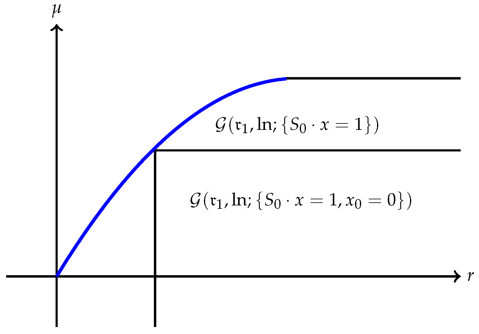
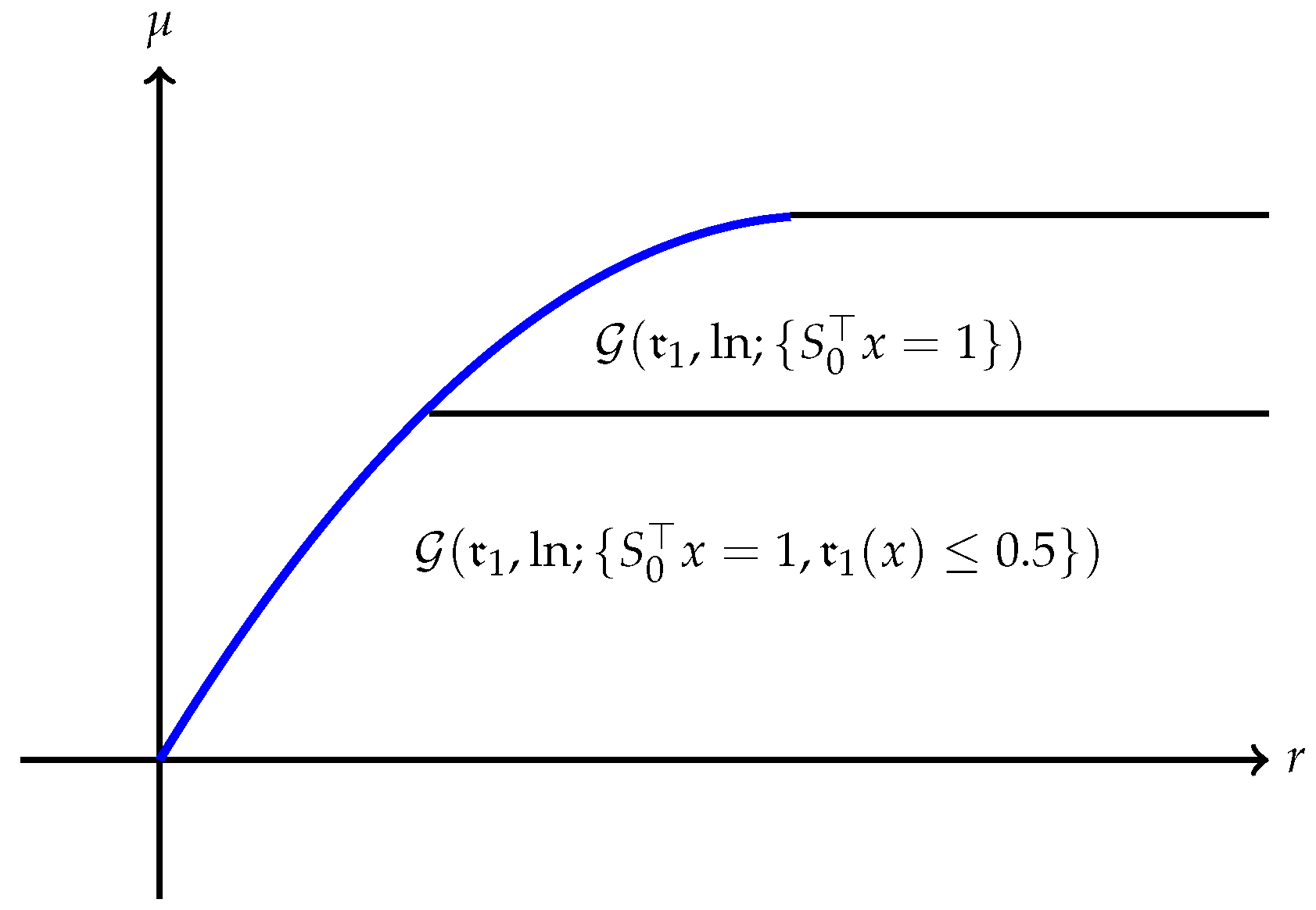
Several interesting cases when has finite endpoints are discussed below:
(a) The quantity is always finite and may be finite as well as illustrated in Figure 1. However, may also be , as Example 1 shows. A typical efficient frontier corresponding to this case is illustrated in Figure 2.
(b) Suppose is finite and attained at an efficient portfolio . Under the conditions of Theorem 5, the portfolio is unique and independent of the risk measure. A graphic illustration is given in Figure 3.
(c) Trade-off between utility and risk is thus implemented by portfolios that trace out a curve in the so-called leverage space introduced by Vince (2009). Note that the curve depends on the risk measure as well as the utility function u. This provides a method for systematically selecting portfolios in the leverage space to reduce risk exposure.
(d) If, in addition, satisfies (r1n) in Assumption 2 and then , and (see Figure 4).
(e) Unlike in (b), finite can also happen when the efficient frontier is unbounded (see Example 2).
Example 1.
(for ) Consider a portfolio problem with the log utility on a financial market that contains no bond and two risky assests (i.e., )
The financial market (since the riskless asset is not involved in (36), it is irrelevant to the problem) is specified as follows: , is a random vector on the sample space with and a payoff matrix
Note that, for instance with , this market has no nontrivial riskless portfolio. We use the risk measure
which satisfies (r1), (r1n) and (r3s) and, therefore, Assumption 4(b) holds. Clearly, and finite. Notice that on the feasible set , i.e., . It follows that the risk measure
attains a minimum at . Observing , we must have and
Example 2.
(for and ) Consider the same risk measure as in the previous example, but use instead the utility function . We analyze
where the financial market is defined by
on the sample space with . Again, on the feasible set , i.e., . The portfolio as a function of implies
As , we can see that and . Hence, and . Notice that (40) with, e.g., , has an arbitrage portfolio , but the existence of an arbitrage seems to be necessary in constructing such an example.
4. Markowitz Portfolio Theory and CAPM Model
Let us now turn to applications of the general theory. We show that the results in the previous section provide a general unified framework for several familiar portfolio theories. They are Markowitz portfolio theory, the CAPM model, growth optimal portfolio theory and leverage space portfolio theory. Of course, when dealing with concrete risk measures and expected utilities related to these concrete theories, an additional helpful structure in the solutions often emerge. Although many different expositions of these theories do already exist in the literature, for the convenience of readers, we include brief arguments using Lagrange multiplier methods. In this entire section, we will assume that the market from Definition 1 has no nontrivial riskless portfolio.
4.1. Markowitz Portfolio Theory
Markowitz portfolio theory that considers only risky assets (see Markowitz (1959)), can be understood as a special case of the framework discussed in Section 3. The risk measure is the standard deviation and the utility function is the identity function. Thus, we face the problem
We assume is not proportional to , that is, for any ,
Since the variance is a monotone increasing function of the standard deviation, we can minimize half of the variance for convenience:
Optimization problem (43) is already in the form (19) with . We can check if condition (c1) in Theorem 5 is satisfied. Moreover, Corollary 1 implies that is positive definite since has no nontrivial riskless portfolio. Hence, the risk function has compact level sets. Thus, Assumption 4 is satisfied and Theorem 5 is applicable. Let be the optimal portfolio corresponding to . Consider the Lagrangian
where . Thanks to Theorem 1, we have
In other words,
We must have because otherwise would be unrelated to the payoff . The complementary slackness condition implies that . Left multiplying (45) by we have
To determine the Lagrange multipliers, we need the numbers , and . Left multiplying (46) by and , we have
and
Solving (48) and (49), we derive
where
since is positive definite and condition (42) holds. Substituting (50) into (47), we see that the efficient frontier is determined by the curve
usually referred to as the Markowitz bullet due to its shape. A typical Markowitz bullet is shown in Figure 5 with an asymptote
Note that . Thus, relationships (52) and (53) describe the efficient frontier as in Definition 5. In addition, note that (52) implies that and . Thus, as a corollary of Theorem 5, we have
Theorem 6.
(Markowitz Portfolio Theorem) Assume that the financial market has no nontrivial riskless portfolio and is not proportional to (see (42)). The Markowitz efficient portfolios of (41) represented in the -plane are given by
They correspond to the upper boundary of the Markowitz bullet given by
The structure of the optimal portfolio in (54) implies the well known two fund theorem derived by Tobin (1958).
Theorem 7.
(Two Fund Theorem) Select two distinct portfolios on the Markowitz efficient frontier. Then, any portfolio on the Markowitz efficient frontier can be represented as the linear combination of these two portfolios.
4.2. Capital Asset Pricing Model
The capital asset pricing model (CAPM) is a theoretical equilibrium model independently proposed by Lintner (1965), Mossin (1966), Sharpe (1964) and Treynor (1999) for pricing a risky asset according to its expected payoff and market risk, often referred to as the beta. The core of the capital asset pricing model is including a riskless bond in the Markowitz mean-variance analysis. Thus, we can apply the general framework in Section 3 with the same setting as in Section 4.1. Similar to the previous section, we can consider the equivalent problem of
Similar to the last section problem (55) is in the form (19) with . We can check that condition (c1) in Theorem 5 is satisfied. Again, the risk function has compact level sets since is positive definite. Thus, Assumption 4 is satisfied and Theorem 5 is applicable. The Lagrangian of this convex programming problem is
where . Again, we have
Clearly, for . Using the complementary slackness condition we derive
by left multiplying in (59). Solving from (59), we have
Left multiplying with and and using the and introduced in the previous section, we derive
and
respectively. Multiplying (63) by R and subtracting it from (62), we get
Clearly, efficient portfolios only occur for , since, for , the pure bond portfolio is the only efficient (and risk free) portfolio. Relation (65) defines a straight line on the -plane
where if
since is positive definite. The line given in (66) is called the capital market line.
Again, we see the affine structure of the solution. Note that, although the computation is done in terms of the risk function , relationships in (66) are in terms the risk function . Thus, they describe the efficient frontier as in Definition 5. In summary, we have
Theorem 8.
(CAPM) Assume that the financial market of Definition 1 has no nontrivial riskless portfolio. Moreover, assume that condition (67) holds. The efficient portfolios for the CAPM model represented in the -plane are a straight line passing through corresponding to the portfolio of pure risk free bond. The optimal portfolio can be determined by (68), which is affine in μ and can be represented as points in the -plane as located on the capital market line
In particular, when and we derive, respectively, the portfolio that contains only the riskless bond and the portfolio that contains only risky assets. We call this portfolio the market portfolio and denote it . The market portfolio corresponds to the coordinates
Since the risk is non negative, we see that the market portfolio exists only when
This condition is
By Theorem 3,
Thus, the market portfolio has to reside on the Markowitz efficient frontier. Moreover, by (68), we can see that the market portfolio is the only portfolio on the CAPM efficient frontier that consists of purely risky assets. Thus,
so that the capital market line is tangent to the Markowitz bullet at as illustrated in Figure 6.
Remark 8.
The affine structure of the solutions is summarized in the following one fund theorem Sharpe (1964); Tobin (1958).
Theorem 9.
(One Fund Theorem) Assume that the financial market has no nontrivial riskless portfolio. Moreover, assume that condition (70) holds. All the optimal portfolios in the CAPM model (55) are generalized convex combinations of the riskless bond and the market portfolio , which corresponds to . The capital market line is tangent to the boundary of the Markowitz bullet at the coordinates of the market portfolio and intercepts the μ-axis at (see Figure 6).
Alternatively, we can write the slope of the capital market line as
This quantity is called the price of risk and we can rewrite the equation for the capital market line (66) as
5. Affine Efficient Frontier for Positive Homogeneous Risk Measure
The affine dependence of the efficient portfolio on the return observed in the CAPM still holds when the standard deviation is replaced by the more general deviation measure (see Rockafellar et al. (2006)). In this section, we derive this affine structure using the general framework discussed in Section 3 and provide a proof different from that of Rockafellar et al. (2006). Moreover, we provide a sufficient condition for the existence of the master fund in the one fund theorem generalizing condition (see (70)) for the existence of the market portfolio in the CAPM model. We also construct a counter-example showing that the two fund theorem (Theorem 7) fails in this setting. Let us consider a risk measure that satisfies (r1), (r1n), (r2) and (r3) in Assumption 2 and the related problem of finding efficient portfolios becomes
Since, for , there is an obvious solution corresponding to , we have and . In what follows, we will only consider . Moreover, we note that for satisfying the positive homogeneous property (r3) in Assumption 2, implies that
In fact, for any ,
and (76) follows. Now we can state and prove the theorem on affine dependence of the efficient portfolio on the return .
Theorem 10.
(Affine Efficient Frontier for Positive Homogeneous Risk Measures) Assume that the risk measure satisfies assumptions (r1), (r1n), (r2) and (r3) in Assumption 2 with and Assumption 4 (b) holds. Furthermore, assume
Then, there exists an efficient portfolio corresponding to on the efficient frontier for problem (75) such that the efficient frontier for problem (75) in the risk-expected return space is a straight line that passes through the points (0,R) corresponding to a portfolio of pure bond and corresponding to the portfolio , respectively. Moreover, the straight line connecting and in the portfolio space, namely for ,
represents a set of efficient portfolios for (75) that corresponds to
in the risk-expected return space (see Definition 5 and (19)).
Proof.
The Lagrangian of this convex programming problem (75) is
where and .
Condition (78) implies that there exists some , such that . Hence, for any , there exists a portfolio of the form satisfying
because the matrix in (82) is invertible. Thus, for any , Assumption 4 (b) with and condition (78) ensure the existence of an optimal solution to problem (75).
Denoting one of those solutions by (may not be unique), we have
Fixing , denote . Then,
Since is independent of , we have
so that, for all ,
because, at the optimal solution the constraint is binding. Using (r3), it follows from (76) and (86) that
Thus, we can write (87) as
For define the homotopy between and
We can verify that and so that
On the other hand, it follows from assumptions (r1) and (r3) that
For any , letting , we have and hence . Thus, by inequality (93), we have . On the other hand, is an efficient portfolio implies that yielding equality
In other words, is an affine function in . In addition, we conclude that points on this efficient frontier correspond to efficient portfolios
as an affine mapping of the parameter into the portfolio space showing (79).
In addition, using we can write (94) as
Corollary 3.
In Theorem 10, if instead of (r3) the stronger condition (r3s) holds, then the portfolio constructed there is unique and, therefore, for each fixed , the efficient portfolio in (79) is unique.
Proof.
Apply Theorem 5 with condition (c3). ☐
Theorem 10 and Corollary 3 manifest a full generalization of Theorem 8 on the capital market pricing model to positive homogeneous risk measures. Note that the necessary conditions on the financial market in (67) and (78) are the same.
Remark 9.
(a) Clearly, corresponds to the portfolio with . If , setting and we see that on the efficient frontier corresponds to a purely risky efficient portfolio of (75)
Since belongs to the image of the affine mapping in (95), the family of efficient portfolios as described by the affine mapping in (95) contains both the pure bond and the portfolio that consists only of purely risky assets. In fact, we can represent the affine mapping in (95) as a parametrized line passing through and as
which is a similar representation of the efficient portfolios as (79). The portfolio is called a master fund in Rockafellar et al. (2006). When , it is the market portfolio in the CAPM. For a general risk measure satisfying conditions (r1), (r1n), (r2) and (r3) in Assumption 2, the master funds are not necessarily unique. However, all master funds correspond to the same point in the risk-expected return space.
(b) We can also consider problem (75) on the set of admissible portfolios of purely risky assets, namely . Then, similar to the relationship between the Markowitz efficient frontier and the capital market line, it follows from Theorem 10 that
as illustrated in Figure 7.
(c) If , then the efficient portfolios in (79) are related to μ in a much simpler fashion
There is no master fund as observed in Rockafellar et al. (2006) in this case. In the language of Rockafellar et al. (2006), the portfolio is called a basic fund. Thus, Theorem 10 recovers the results in Theorem 2 and Theorem 3 in Rockafellar et al. (2006) with a different proof and a weaker condition (condition (78) is weaker than (A2) on page 752 of Rockafellar et al.). However, Corollary 3 is a significant improvement yielding uniqueness in case (r3s) holds. This will help below when we derive a sufficient condition for the existence of a master fund, which is solely depending on the risk measure and the financial market.
We see in Remark 9 that the existence of a master fund depends on whether or not . Below, we characterize this condition in terms of and its Fenchel conjugate , defined by .
Theorem 11.
Under the conditions of Corollary 3, assuming that is differentiable at , a master fund exists if and only if .
Proof.
By virtue of the Fenchel–Young equality (see (Carr and Zhu forthcoming, Proposition 1.3.1)), we have
and
It follows that is equivalent to
The last equality is because implies . ☐
Remark 10.
We refer to Borwein and Vanderwerff (2009) for conditions ensuring the differentiability of in Theorem 11. In the CAPM model and . Thus, the master fund exists if and only if
which exactly recovers the condition in (70) for the existence of a market portfolio in the one fund theorem (cf. Theorem 9).
In general, for a risk measure with (r1), (r1n) and (r3s), if is , then where is the Hessian of f at . Thus, a criterion for the existence of a master fund similar to (70) holds with Σ replaced by .
Another very useful case is . It is not hard to show that the conjugate of is . In fact, it follows from the Cauchy inequality that Thus,
On the other hand, for any , defining , we have
The maximum of the expression in (106) as a function of t is . It follows that
Combining (105) and (107), we arrive at . This example illustrates that using and its conjugate often helps. In fact, is differentiable everywhere except for the coordinate axises. However, is an indicator function on the closed set (see (Carr and Zhu forthcoming), Proposition 2.4.2)), whose derivative is 0 at any differentiable point and, therefore, is not useful for our purpose.
Since the standard deviation satisfies Assumptions (r1), (r1n), (r2) and (r3s), the result above is a generalization of the relationship between the CAPM model and the Markowitz portfolio theory. We note that the standard deviation is not the only risk measure that satisfies these assumptions. For example, some forms of approximation to the expected drawdowns also satisfy these assumptions (cf. Maier-Paape and Zhu (2017)).
Theorem 10 and Corollary 3 are a full generalization of Theorem 8 on the CAPM and Theorem 11 is a generalization of the one fund theorem in Theorem 9. On the other hand, in Rockafellar et al. (2006), footnote 10, it has been noted that a similar generalization of the two fund theorem (Theorem 7) is not to be expected. We construct a concrete counter-example below.
Example 3.
(Counter-example to a Generalized Two Fund Theorem) Let us consider, for example,
with .
Choose all , so that is . Choose the payoff such that so that at the optimal solution. Finally, let us construct so that the optimal solution is not affine in μ.
We do so by constructing a convex set G with (interior of G) and then set for (boundary of G) and extend to be positive homogeneous. Then, (r1), (r1n), (r2) and (r3) are satisfied.
Now, let us specify G. Take the convex hull of the set and five other points. One point is and the other four points and D, are the corner points of a square that lies in the plane and has unit side length. To obtain that square, take the standard square with unit side length in , i.e., the square with corner points and rotate this square by 30 degrees counter clockwise in the -plane. Doing some calculation, one gets:
Obviously for the optimal solution is with . For with small, we have (they lie on the ray through a point on the convex combination of C and ), and, for with large, we have (they lie on the ray through a point on the set . Therefore, cannot be affine in μ.
6. Growth Optimal and Leverage Space Portfolio
Growth portfolio theory is proposed by Lintner (1965) and is also related to the work of Kelly (1956). It is equivalent to maximizing the expected log utility:
Remark 11.
Problem (109) is equivalent to
The following theorem establishes the existence of the growth optimal portfolio as a corollary of our results in Section 3. This theorem reconfirms previous results in Hermes and Maier-Paape (2017) with somewhat different conditions and a shorter proof.
Theorem 12.
(Growth Optimal Portfolio) Assume that the financial market of Definition 1 has no nontrivial riskless portfolio. Then, problem (109) has a unique optimal portfolio, which is often referred to as the growth optimal portfolio and is denoted .
To prove Theorem 12, we need the following lemma.
Lemma 2.
Assume that the financial market of Definition 1 has no nontrivial riskless portfolio. Let u be a utility function satisfying (u3) in Assumption 3. Then, for any ,
is compact (and possibly empty in some cases).
Proof.
Since, by Assumption 3, u is upper semi-continuous, the set in (111) is closed. Thus, we need only to show it is also bounded. Assume the contrary that there exists a sequence of portfolios with
and satisfying
Proof of Theorem 12.
Assuming one repeatedly invests in the identical one period financial market, the growth optimal portfolio has the nice property that it provides the fastest compounded growth of the capital. By Remark 7(b), it is independent of any risk measures. In the special case that all the risky assets are representing a certain gaming outcome, is the Kelly allocation in Kelly (1956). However, the growth portfolio is seldomly used in investment practice for being too risky. The book (MacLean et al.2009) provides an excellent collection of papers with chronological research on this subject. These observations motivated Vince (2009) to introduce his leverage space portfolio to scale back from the growth optimal portfolio. Recently, De Prado et al. (2013); Vince and Zhu (2015) further introduce systematical methods to scale back from the growth optimal portfolio by, among other ideas, explicitly accounting for limiting a certain risk measure. The analysis in Vince and Zhu (2015) and De Prado et al. (2013) can be phrased as solving
where is a risk measure that satisfies conditions (r1) and (r2). Alternatively, to derive the efficient frontier, we can also consider
Applying Proposition 8, Theorem 5 and Remark 7 to the set of admissible portfolios , we derive:
Theorem 13.
(Leverage Space Portfolio and Risk Measure) We assume that the financial market in Definition 1 has no nontrivial riskless portfolio and that the risk measure satisfies conditions (r1), (r1n) and (r2). Then, the problem
has a bounded efficient frontier that can be parameterized as follows:
Proof.
Note that Assumption 4 (a) holds due to Lemma 2 and (c2) in Theorem 5 is also satisfied. Then, (a) follows straightforwardly from Theorem 5, where and are finite and attained and (b) follows from Theorem 5 with and . ☐
Remark 12.
Theorem 13 relates the leverage portfolio space theory to the framework setup in Section 3. It becomes clear that each risk measure satisfying conditions (r1), (r1n) and (r2) generates a path in the leverage portfolio space connecting the portfolio of a pure riskless bond to the growth optimal portfolio. Theorem 13 also tells us that different risk measures usually correspond to different paths in the portfolio space. Many commonly used risk measures satisfy conditions (r1) and (r2). The curve provides a pathway to reduce risk exposure along the efficient frontier in the risk-expected log utility space. As observed in De Prado et al. (2013); Vince and Zhu (2015), when investments have only a finite time horizon, then there are additional interesting points along the path such as the inflection point and the point that maximizes the return/risk ratio. Both of which provide further landmarks for investors.
Similar to the previous sections, we can also consider the related problem of using only portfolios involving risky assets, i.e.,
Theorem 14.
(Existence of Solutions) Suppose that
Then, problem (119) has a solution.
Proof.
As in the proof of Theorem 13, we can see that Assumption 4 (a) holds due to Lemma 2. Observe that, for , we get from (120) that is finite. Then, we can directly apply Theorem 5 with . ☐
With the help of Theorem 14, we can conclude that problem
generates an efficient frontier as well (comparable to the Markowitz bullet for ). However, due to the involvement of the log utility function, the relative location of efficient frontiers stemming from (118) and (121) may have several different configurations. The following is an example.
Example 4.
Let . Consider a sample space with probability and and a financial market involving a riskless bond with and one risky asset specified by , and with so that . Use the risk measure (which is an approximation of the drawdown cf. Vince and Zhu (2015)). Then, it is easy to calculate that the efficient frontier corresponding to (118) is
where . On the other hand, the efficient frontier stemming from (121) is a single point where .
Remark 13.
(Efficiency Index) Although the growth optimal portfolio is usually not implemented as an investment strategy, the maximum utility corresponding to the growth optimal portfolio κ, empirically estimated using historical performance data, can be used as a measure to compare different investment strategies. This is proposed in Zhu (2007) and called the efficiency index. When the only risky asset is the payoff of a game with two outcomes following a given playing strategy, the efficiency coefficient coincides with Shannon’s information rate (see Kelly (1956); Shannon and Weaver (1949); Zhu (2007)). In this sense, the efficiency index gauges the useful information contained in the investment strategy it measures.
7. Conclusions
Following the pioneering idea of Markowitz to trade-off the expected return and standard deviation of a portfolio, we consider a general framework to efficiently trade-off between a concave expected utility and a convex risk measure for portfolios. Under reasonable assumptions, we show that (i) the efficient frontier in such a trade-off is a convex curve in the expected utility-risk space, (ii) the optimal portfolio corresponding to each level of the expected utility is unique and (iii) the optimal portfolios continuously depend on the level of the expected utility. Moreover, we provide an alternative treatment and enhancement of the results in Rockafellar et al. (2006) showing that the one fund theorem (Theorem 9) holds in the trade-off between a deviation measure and the expected return (Theorem 11) and construct a counter-example illustrating that the two fund theorem (Theorem 7) fails in such a general setting. Furthermore, the efficiency curve in the leverage space is supposedly an economic way to scale back risk from the growth optimal portfolio (Theorem 13).
This general framework unifies a group of well known portfolio theories. They are Markowitz portfolio theory, capital asset pricing model, the growth optimal portfolio theory, and the leverage portfolio theory. It also extends these portfolio theories to more general settings.
The new framework also leads to many questions of practical significance worthy of further explorations. For example, quantities related to portfolio theories such as the Sharpe ratio and efficiency index can be used to measure investment performances. What other performance measurements can be derived using the general framework in Section 3? Portfolio theory can also inform us about pricing mechanisms such as those discussed in the capital asset pricing model and the fundamental theorem of asset pricing (see (Carr and Zhu forthcoming, Section 2.3). What additional pricing tools can be derived from our general framework?
Clearly, for the purpose of applications, we need to focus on certain special cases. Drawdown related risk measures coupled with the log utility attracts much attention in practice. In Part II of this series Maier-Paape and Zhu (2017), several drawdown related risk measures are constructed and analyzed.
Author Contributions
S.M.-P. and Q.J.Z. contributed equally to the work reported.
Acknowledgments
We thank Andreas Platen for his constructive suggestions after reading earlier versions of the manuscript.
Conflicts of Interest
The authors declare no conflict of interest.
References
- Artzner, Philippe, Freddy Delbaen, Jean-Marc Eber, and Davia Heath. 1999. Coherent measures of risk. Mathematical Finance 9: 203–27. [Google Scholar] [CrossRef]
- Borwein, Jonathan M., and Jon Vanderwerff. 2009. Differentiability of conjugate functions and perturbed minimization principles. Journal of Convex Analysis 16: 707–11. [Google Scholar]
- Borwein, Jonathan M., and Qiji Jim Zhu. 2005. Techniques of Variational Analysis. New York: Springer. [Google Scholar]
- Borwein, Jonathan M., and Qiji Jim Zhu. 2016. A variational approach to Lagrange multipliers. Journal of Optimization Theory and Applications 171: 727–56. [Google Scholar] [CrossRef]
- Carr, Peter, and Qiji Jim Zhu. Forthcoming. Convex Duality and Financial Mathematics. Berlin: Springer.
- De Prado, Marcos Lopez, Ralph Vince, and Qiji Jim Zhu. 2013. Optimal risk budgeting under a finite investment horizon. SSRN Electronic Journal, 2364092. Available online: https://ssrn.com/abstract=2364092 (accessed on 29 March 2018).
- Hermes, Andreas, and Stanislaus Maier-Paape. 2017. Existence and Uniqueness for the Multivariate Discrete Terminal Wealth Relative. Risks 5: 44. [Google Scholar] [CrossRef]
- Kelly, John L. 1956. A new interpretation of information rate. Bell System Technical Journal 35: 917–26. [Google Scholar] [CrossRef]
- Lintner, John. 1965. The valuation of risk assets and the selection of risky investments in stock portfolios and capital budgets. Review of Economics and Statistics 47: 13–37. [Google Scholar] [CrossRef]
- MacLean, Leonard C., Edward O. Thorp, and William T. Ziemba, eds. 2009. The Kelly Capital Growth Criterion: Theory and Practice. Singapore: World Scientific. [Google Scholar]
- Maier-Paape, Stanislaus. 2015. Optimal f and diversification. International Federation of Technical Analysts Journal 15: 4–7. [Google Scholar]
- Maier-Paape, Stanislaus. 2016. Risk Averse Fractional Trading Using the Current Drawdown. Report No. 88. Aachen: Institut für Mathematik, RWTH Aachen. [Google Scholar]
- Maier-Paape, Stanislaus, and Qiji Jim Zhu. 2017. A General Framework for Portfolio Theory. Part II: Drawdown Risk Measures. Report No. 92. Aachen: Institut für Mathematik, RWTH Aachen. [Google Scholar]
- Markowitz, Harry. 1959. Portfolio Selection. Cowles Monograph, 16. New York: Wiley. [Google Scholar]
- Mossin, Jan. 1966. Equilibrium in a Capital Asset Market. Econometrica 34: 768–83. [Google Scholar] [CrossRef]
- Rockafellar, Ralph Tyrell. 1970. Convex Analysis. Vol. 28 Princeton Math. Series; Princeton: Princeton University Press. [Google Scholar]
- Rockafellar, R. Tyrrell, and Stanislav Uryasev. 2000. Optimization of conditional value-at-risk. Journal of Risk 2: 21–42. [Google Scholar] [CrossRef]
- Rockafellar, R. Tyrrell, Stan Uryasev, and Michael Zabarankin. 2006. Master funds in portfolio analysis with general deviation measures. Journal of Banking and Finance 30: 743–78. [Google Scholar] [CrossRef]
- Shannon, Claude E., and Warren Weaver. 1949. The Mathematical Theory of Communication. Urbana: University of Illinois Press. [Google Scholar]
- Sharpe, William F. 1964. Capital asset prices: A theory of market equilibrium under conditions of risk. Journal of Finance 19: 425–42. [Google Scholar]
- Sharpe, William F. 1966. Mutual fund performance. Journal of Business 1: 119–38. [Google Scholar] [CrossRef]
- Tobin, James. 1958. Liquidity preference as behavior towards risk. The Review of Economic Studies 26: 65–86. [Google Scholar] [CrossRef]
- Treynor, Jack L. 1999. Toward a theory of market value of risky assets. In Asset Pricing and Portfolio Performance: Models, Strategy and Performance Metrics. Edited by Robert A. Korajczyk. London: Risk Books, pp. 15–22. [Google Scholar]
- Vince, Ralph. 2009. The Leverage Space Trading Model. Hoboken: John Wiley and Sons. [Google Scholar]
- Vince, Ralph, and Qiji Jim Zhu. 2015. Optimal betting sizes for the game of blackjack. Risk Journals: Portfolio Management 4: 53–75. [Google Scholar] [CrossRef]
- Zhu, Qiji Jim. 2007. Mathematical analysis of investment systems. Journal of Mathematical Analysis and Applications 326: 708–20. [Google Scholar] [CrossRef]
Figure 1.
Efficient frontier with both and are finite and attained.

Figure 2.
Efficient frontier with .

Figure 3.
Efficient frontier when and is finite and attained as maximum.
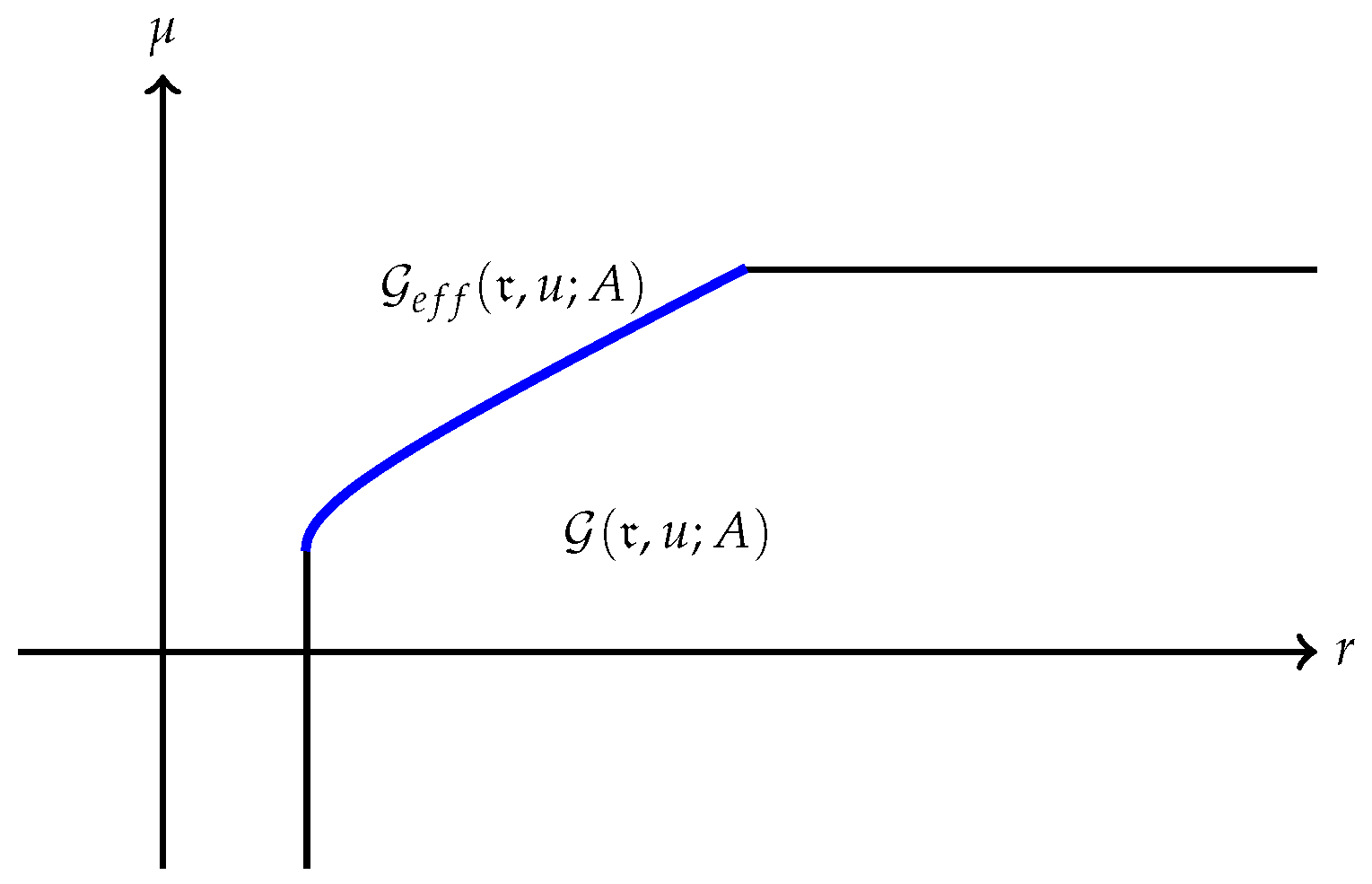
Figure 4.
Efficient frontier with .
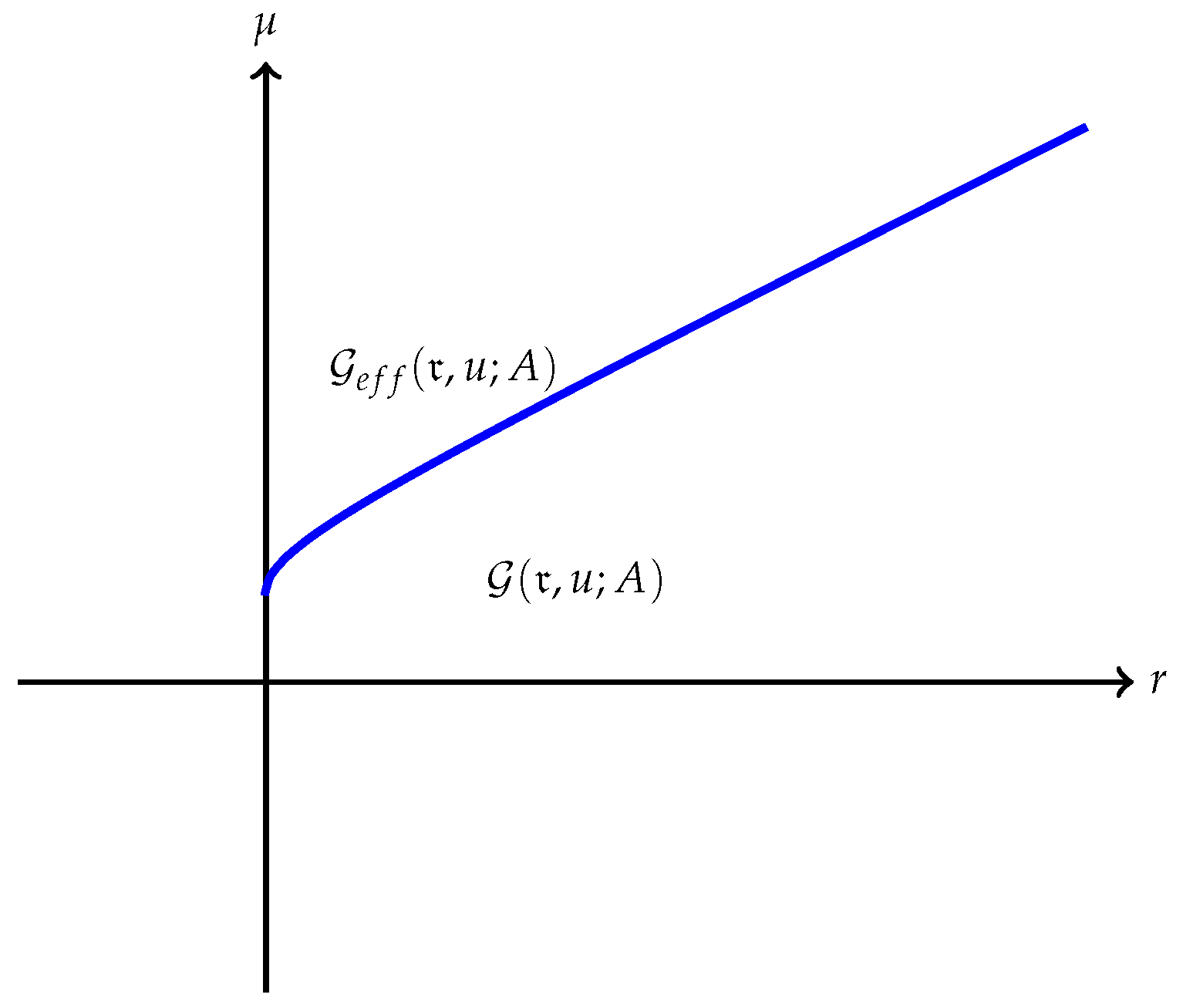
Figure 5.
Markowitz Bullet.
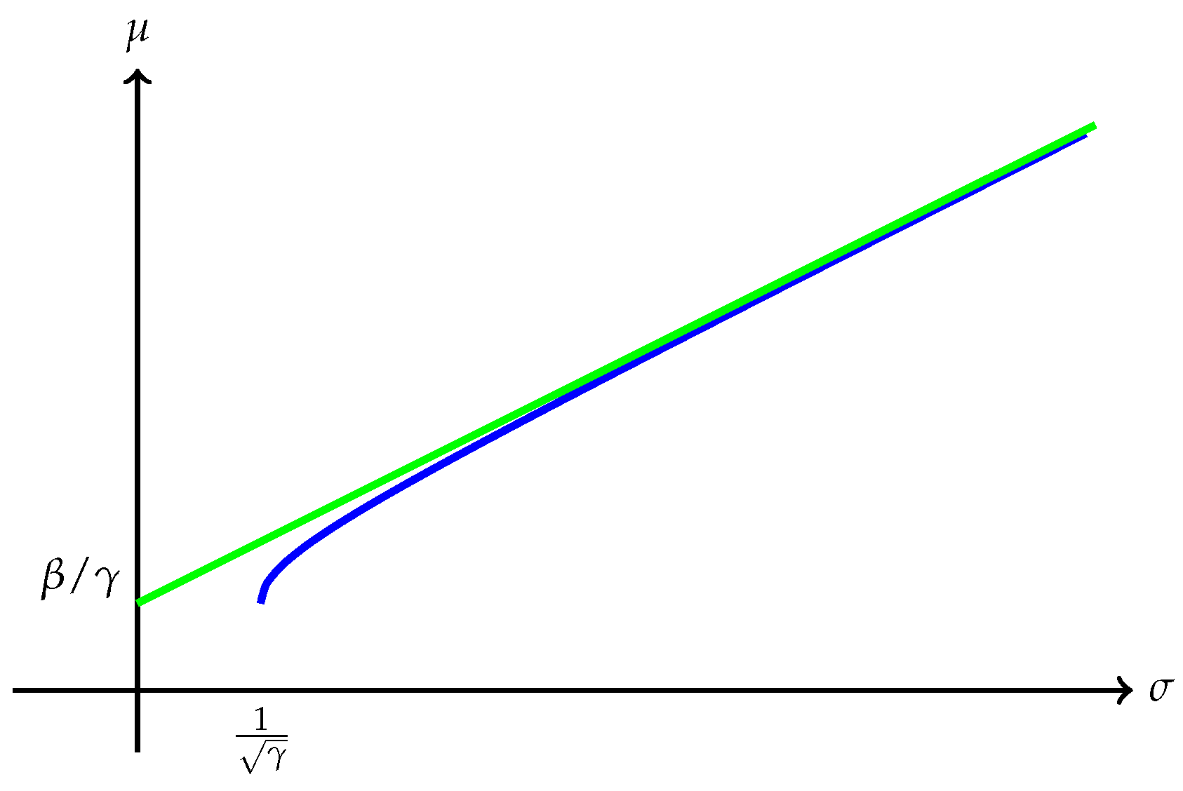
Figure 6.
Capital Market Line and Markowitz Bullet.
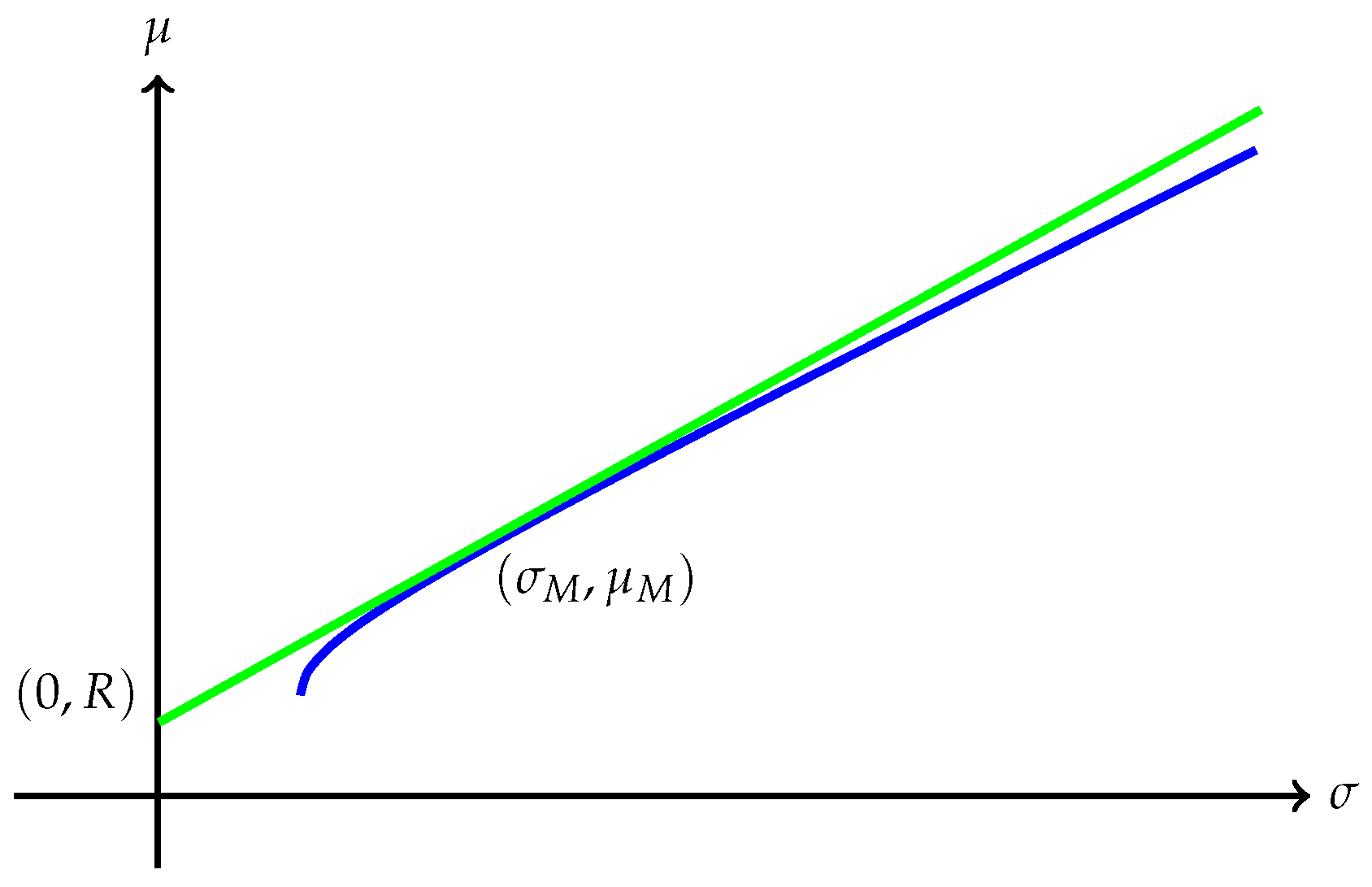
Figure 7.
Capital Market Line for (75) when .
Figure 7.
Capital Market Line for (75) when .

Figure 8.
Separated efficient frontiers.

Figure 9.
Touching efficient frontiers.

Figure 10.
Touching efficient frontiers at growth optimal.
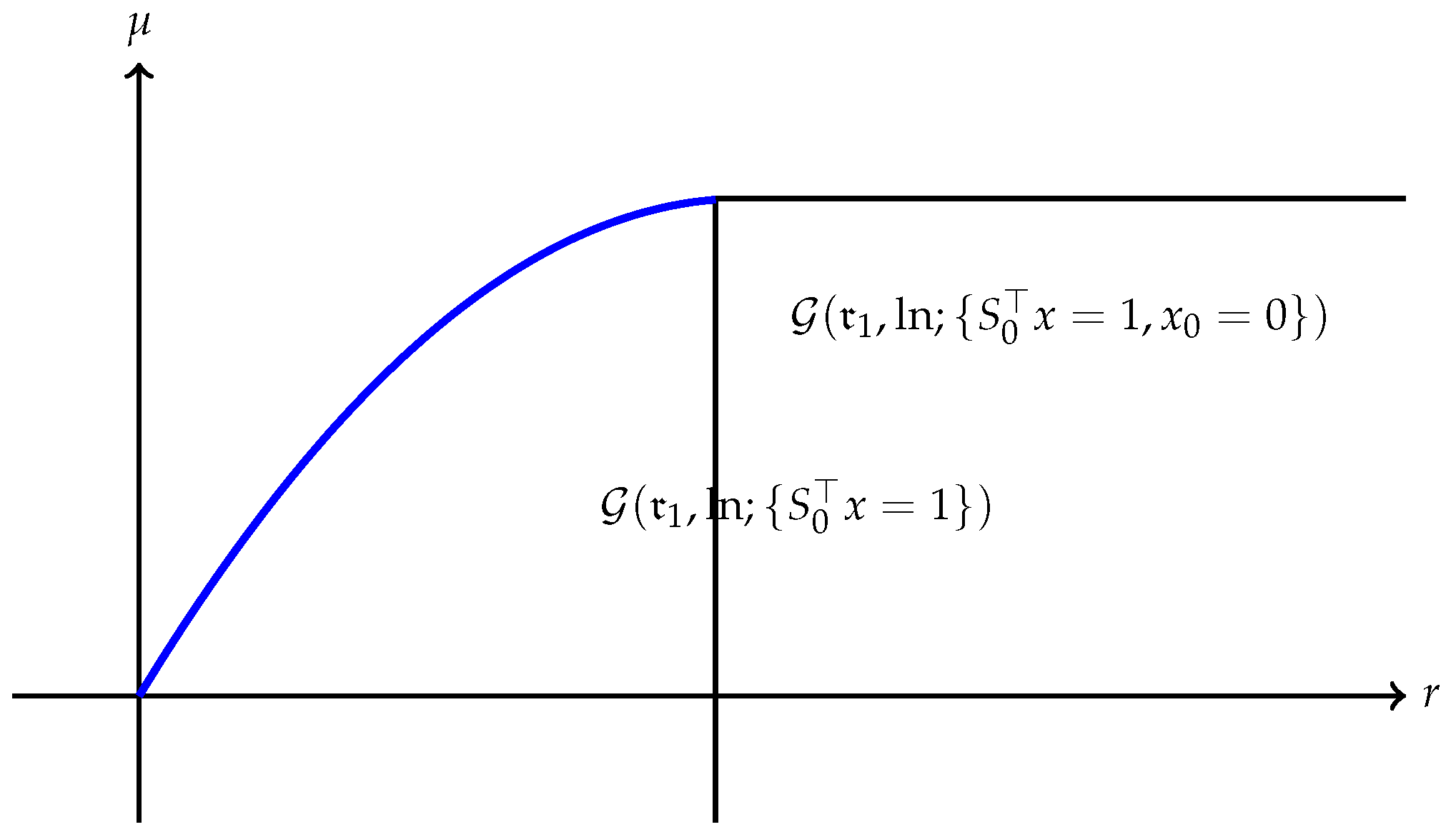
Figure 11.
Shared efficient frontiers.

© 2018 by the authors. Licensee MDPI, Basel, Switzerland. This article is an open access article distributed under the terms and conditions of the Creative Commons Attribution (CC BY) license (http://creativecommons.org/licenses/by/4.0/).
Share and Cite
MDPI and ACS Style
Maier-Paape, S.; Zhu, Q.J. A General Framework for Portfolio Theory—Part I: Theory and Various Models. Risks 2018, 6, 53. https://doi.org/10.3390/risks6020053
AMA Style
Maier-Paape S, Zhu QJ. A General Framework for Portfolio Theory—Part I: Theory and Various Models. Risks. 2018; 6(2):53. https://doi.org/10.3390/risks6020053
Chicago/Turabian StyleMaier-Paape, Stanislaus, and Qiji Jim Zhu. 2018. "A General Framework for Portfolio Theory—Part I: Theory and Various Models" Risks 6, no. 2: 53. https://doi.org/10.3390/risks6020053
Note that from the first issue of 2016, this journal uses article numbers instead of page numbers. See further details here.