1. Introduction
“Can we trust chain-ladder models?” is a central question in non-life insurance claim reserving. It hinges on the model assumptions: if these are violated the answer would be “no”. For example, the popular over-dispersed Poisson chain-ladder model assumes a fixed variance to mean ratio across the run-off triangle. If this is false then distribution forecasts are bound to fail. Yet, there is no statistical theory available to test for a violation of this assumption.
We show that testing for a violation of central assumptions is straightforward in two popular chain-ladder models: over-dispersed Poisson and log-normal. While the over-dispersed Poisson model assumes a fixed variance to mean ratio, the log-normal model imposes a common variance of the log data. Further, both models assume a chain-ladder structure. That is, accident year effects do not vary by development year and vice versa. We show that these assumptions are not only testable, but testable with standard tools that can easily be implemented in a spreadsheet.
The over-dispersed Poisson model arguably owes its special status to the ubiquitous chain-ladder technique.
Kremer (
1985) showed that this deterministic technique so commonly used in claim reserving is replicated by maximum likelihood estimation in a Poisson model. However, integer support and the implicit assumption that the variance equals the mean cannot be reconciled with insurance claim data. This explains the need for the over-dispersed Poisson model which relaxes both of these assumptions. Unlike the Poisson model, the over-dispersed Poisson model is moment-based and does not come equipped with a distributional framework. Despite this shortcoming, distribution forecasts are needed and bootstrapping (
England 2002;
England and Verrall 1999) is in widespread use. Yet, so far we do not have a statistical theory for the bootstrap in this setting.
Recently,
Harnau and Nielsen (
2017) proposed a distributional framework that incorporates the moment assumptions of the over-dispersed Poisson model. This framework allows for a compelling asymptotic theory that does not require a large array but rather large cell means. The practical implication is that for a run-off triangle with a large, potentially unknown, number of payments, we can use a fixed sample size Gaussian distribution theory. They derive parameter distributions, tests for model reduction, such as the absence of calendar effects, and closed form distribution forecasts. Their assumptions accommodate, among others, many compound Poisson distributions. In insurance, these have the interpretation that each cell of aggregate incremental claims is the sum of a Poisson number of claims each with a random individual claim amount. The asymptotic theory then does not assume that we have many such cells, but rather that the mean of the Poisson number of claims is large. We stress that while
Harnau and Nielsen (
2017) largely use terminology from the age-period-cohort literature, the theory immediately applies to the reserving literature by renaming age, period, and cohort effects to development, calendar, and accident effects.
Modeling aggregate incremental claims as log-normal rather than over-dispersed Poisson is also common.
Kremer (
1982) introduced a log-normal model with multiplicative mean structure mirroring the over-dispersed Poisson chain-ladder model. While this model does not replicate the classic chain-ladder technique, it is easily estimated by least squares. Recently,
Kuang et al. (
2015) derived explicit expression for the estimators in the log-normal model. These have interpretation as a geometric, rather than the classic arithmetic chain ladder. Other contributions for the log-normal model are discussed in the excellent overview of stochastic reserving models by
England and Verrall (
2002).
We are of course not the first to question the validity of the assumptions in these models. Yet, so far the problem was dealt with by specifying more flexible models. For example,
Hertig (
1983) considers a log-normal model that allows the log data variance to vary by development year. The double-chain-ladder model by
Martínez Miranda et al. (
2012) has, conditional on the incurred counts, an approximate over-dispersed Poisson structure where the over-dispersion varies by accident year. The “distribution-free” model by
Mack (
1993) has separate variance parameters for each development year. We note that while this model also replicates the classical chain-ladder point forecasts, it differs from the over-dispersed Poisson model and so far lacks a distributional framework that would allow for a rigorous statistical theory. Thus, while it is a popular model, we do not consider it further in this paper.
While using more flexible models seems sensible when assumptions are violated, we should not be too quick to dispose of well-known simple models. Particularly for forecasting, such simpler models may be advantageous. A statistical framework for misspecification testing is thus needed. The tests may corroborate the initial modeling choice of the expert, draw attention to an issue, or confirm the suspicion that the model is not well suited for the task. Whichever scenario the expert encounters, the misspecification tests can help to make an informed choice.
The test statistics we propose in this paper are well known in an analysis of variance (ANOVA) context. There, the researcher is usually presented with several samples and wants to test for treatment effects. The data are often assumed to be independent Gaussian. The first step is to test for common variances across samples. This is done with a Bartlett test based on an easily computed likelihood ratio statistic. Then, given common variances, a standard F-test can be used to test for different means between the samples, indicating a treatment effect.
The difference to the ANOVA application is that we generally have data for only one sample, often a run-off triangle. We thus reverse engineer the ANOVA situation by splitting the data into several artificial sub-samples. This idea has a long history in the econometric literature. For instance,
Chow (
1960) proposed a test for structural breaks that involved splitting the sample at the known breakpoint. In the (weak) instrumental variable literature,
Angrist and Krueger (
1995) proposed a split-sample procedure with the objective to break the bias of the instrumental variable estimator towards the ordinary least squares estimator.
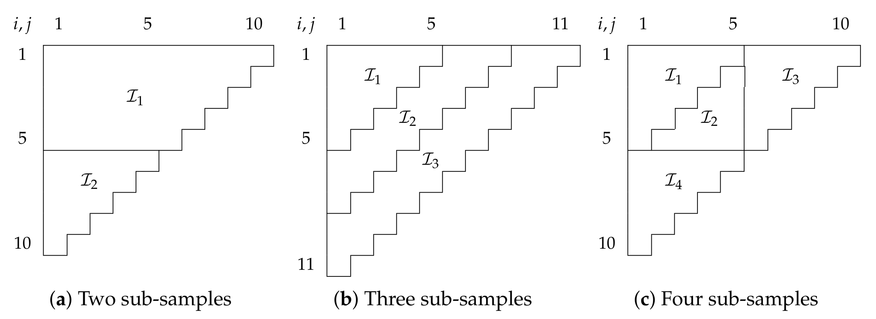
Figure 1 shows examples of how we could split run-off triangles into sub-samples.
In
Section 2, we give a precise definition for the conditions that both the data set as well as the artificial sub-samples must meet. We note that while we do not provide guidance on how to chose the sub-sample structure in this paper, the choice does not affect the size of the proposed tests under the null hypothesis.
In a log-normal model, taking logs yields Gaussian data such that we can directly apply the Bartlett and
F-test from the ANOVA scenario. While the finite sample distribution of the Bartlett test statistic has no closed form, it does not have nuisance parameters and critical values could easily be simulated. However,
Bartlett (
1937) suggests a
approximation to the exact distribution that allows us to sidestep simulations. For a special case with just two sub-samples, we can also apply an
F-test for the hypothesis for common variances of the log data ; while Bartlett and
F-tests are not identical, simulations indicate that they give similar information. Next, we show that an
F-test for common mean parameters is not only straightforward but also independent of the Bartlett test. These results are collected in
Section 3.
In the over-dispersed Poisson model, the asymptotic framework by
Harnau and Nielsen (
2017) catapults us into a finite dimensional Gaussian world. Therefore, the results developed for the log-normal model carry over. We can now asymptotically use a Bartlett test as a test for common over-dispersion across sub-samples. Similarly, an
F-test for common mean parameters across sub-samples is asymptotically F-distributed and asymptotically independent of the dispersion parameter tests. We stress again that the asymptotic theory does not require a large triangle but rather large means of the cells in the triangle. As for the log-normal model, we could simulate critical values for the Bartlett test; however a
approximation can still be justified. We show all this in
Section 4.
The Bartlett test is easily implemented and makes an empirical application straightforward. The same is true for an
F-test on the means. We illustrate the testing procedure, splitting the data, estimating the sub-models, Bartlett testing for common dispersion parameters, and
F-testing for common mean parameters, in
Section 5 with several empirical applications.
We clear up remaining questions about the power of the tests and the performance of approximations in a simulation study based on a run-off triangle. First, it would not take much to simulate critical values of the Bartlett test statistic under the null, rather than to use a
approximation. However, we show in a simulation study that this approximation works so well that simulating critical values seems superfluous. Second, we produce power curves under several alternatives for the test for common variances of the log data in a log-normal model. Third, we find that the asymptotic results for the over-dispersed Poisson model are well approximated in finite samples, at least in our simulations. The simulation study is in
Section 6.
Finally, we discuss some open questions for future research such as how to choose the sub-sample structure and whether one can select between over-dispersed Poisson and log-normal model. With this,
Section 7 concludes the paper.
2. Data and Sub-Samples
Our aim is to test model specification by using statistics that are usually employed to test for common parameters across separate samples. However, we are presented with just a single sample, such as a run-off triangle. Thus, we artificially construct separate samples by splitting the data at hand into sub-samples. Many intuitive splits can be accommodated by the theory, for example, all sub-samples in
Figure 1. Here, we define precisely the permissible structures for data and sub-samples, illustrated on an example of a run-off triangle.
For the theory in this paper, we assume that data are a generalized trapezoid as defined by
Kuang et al. (
2008). This flexible format allows for different numbers of accident and development years, and can accommodate missing past and future calendar years. Run-off triangles are a special case with as many accident as development years and only future calendar years missing. For accident year
i and development year
j, we count calendar years
k with an offset so
. Generalized trapezoids are characterized by the index set
where
and
,
and
, and
and
are the smallest and largest accident, development and calendar year indices available, respectively. We denote the number of cells in
by
n. The run-off triangle in
Table 1, taken from
Taylor and Ashe (
1983), are a generalized trapezoid with
= 1,
and
.
We also assume that each sub-sample is a generalized trapezoid. We denote sub-samples by
. The sub-samples should be disjoint so
and their union should be the original sample so
. All sub-samples of the examples in
Figure 1 are generalized trapezoids. For instance, the sub-sample
in
Figure 1c is specified by
,
,
,
and
.
The purpose of the generalized trapezoid assumption is to ensure parameter identification later on. We note that this assumption is often more restrictive than needed. Examples for arrays that do not fall into the generalized trapezoid category are arrays with missing cells and disconnected arrays such as the combination of sub-samples
and
in
Figure 1b. However, for many of these arrays identification may still be given and then the theory developed below will still be valid.
3. Log-Normal Model
Given data and sub-samples, we can specify a log-normal model, define estimators, and provide the theory for specification testing. The idea is to start with a model that allows parameters to vary across sub-samples and then to test for reductions to a model with common parameters. The latter, most restrictive, model is commonly used in claim reserving. If we reject a reduction to this model, it is likely misspecified. Estimation is done by least squares. The first hypothesis is that log data variances are common across sub-samples; we can test this with a Bartlett test. The second hypothesis is for common linear predictors and can be assessed with an independent F-test.
3.1. Model and Hypotheses
The unrestricted model allows both log data means and variances to vary across sub-samples. For this model, we assume that the aggregate incremental claims
for accident year
i, development year
j, and sub-sample
ℓ are independent log-normal with
While we focus on linear predictors
with accident and development year effect, the theory in this paper allows for more general or restrictive linear predictors. For example, we could incorporate calendar year effects as in
Zehnwirth (
1994) or
Kuang et al. (
2011).
The first hypotheses restricts log data variances to be common across sub-samples
. The remaining assumptions are maintained; thus, linear predictors are still allowed to vary across sub-samples. We write the hypothesis as
The model that arises by imposing this restriction is
The second hypothesis nests the first but also restricts linear predictors to be common across sub-samples. The hypothesis is
Under this hypothesis, all parameters are common across sub-samples
. Thus, we can feasibly drop the sub-script
ℓ and write the model under this hypothesis as
This is the log-normal geometric chain-ladder model.
We can also think about the hypotheses on the original scale. Mean and variance parameters on the log-scale map into median and coefficients of variations on the original scale. Taking the model
under
as an example,
Thus, the separation between mean and variance on the log-scale translates to separation between median and coefficient of variation on the original scale. Hence, we can alternatively think of as the hypothesis of common coefficients of variation and of as further imposing common median parameters.
3.2. Estimation
We estimate on the log-scale with standard estimators, least squares for log data means and residual sum of squares for log data variances. Since the theory for testing developed below is adapted from a Gaussian framework, estimation on the log-scale is intuitive. Before specifying the estimators, we briefly discuss identification.
The identification problem is that
for any
. Thus, the levels of accident and development effects are not identified. However, the linear predictors
are identified (
Kuang et al. 2008). These are thus invariant to the identification constraints imposed on the individual effects. Therefore, it does not matter whether we impose ad-hoc constraints such as
or non ad-hoc constraints as suggested by
Kuang et al. (
2008). We choose to discuss estimation based on the latter, which has the advantage that it allows for straightforward counting of degrees of freedom. By way of example, we apply the identification by
Kuang et al. (
2008) to a run-off triangle with
. Defining the first difference operator as
, the idea is to re-write
Then, where the design vector and the identified parameter vector is . We denote the number of parameters as . The identification method can be extended to generalized trapezoids as well as to linear predictors with calendar year effects.
3.2.1. Estimation in Unrestricted Model
For the unrestricted model
, we estimate linear predictors as
With degrees of freedom
, we estimate log data variances by
3.2.2. Estimation with Common Variances in
Imposing the restriction of common log data variances
does not require re-estimation as the estimators from
can be re-used. The estimators for the linear predictors
are identical to those of
. The log data variance in
is estimated by
where
and
.
3.2.3. Estimation with Common Variances and Linear Predictors in
Under the hypothesis
, which imposes common log data mean and variance parameters, both estimators change. We drop the
ℓ-subscript indicating the sub-sample since estimation is done over the full sample
. With that, we write the estimators for the linear predictors in
as
We estimate the log data variance
under this hypothesis, defining
, by
3.2.4. Remarks
Least squares estimation for the identified parameter vector
is maximum likelihood estimation in the log-normal model.
Kuang et al. (
2015) derive a representation of the least squares estimators that is interpretable as a geometric chain-ladder, in contrast to the classic, arithmetic, chain-ladder.
For many regression models, there is little difference between scaling the residual sum of squares by the degrees of freedom or the number of observations; the former yields an unbiased estimator for
, the latter the maximum likelihood estimator. However, the scaling does matter here due to the large parameter to observation ratio. By way of example, the
Taylor and Ashe (
1983) data has
observations but only
degrees of freedom so that
is some 50% larger then the rival estimator
. This is amplified for the sub-samples.
3.3. Testing for Common Variances
We show how to test for common log data variances, that is for in using a Bartlett test. In a special case with two sub-samples, we can use an F-test instead of a Bartlett test.
The Bartlett test (
Bartlett 1937) was designed to test for common variances across several Gaussian samples. Thus, it is directly applicable to the log sub-samples. We only give a rough overview of the theory; for a more detailed derivation in contemporary terminology see
Jørgensen (
1993, pp. 94–96). The test rests on the independent
-distribution of
in
. Rather than deriving a test in the Gaussian model for
,
Bartlett (
1937) considers a joint
model for the variance estimators. In this
model, the log-likelihood ratio statistic for the hypothesis
is
for
and
as defined in (1) and (2), respectively. Define now the Bartlett distribution
such that
under the hypothesis. Considering
as a function of the estimators so
, the Bartlett distribution is characterized by
where
is the
cdf and
. Likelihood theory tells us that
and thus
approaches a
as
goes to infinity. However,
Bartlett (
1937) goes a step further and suggest to divide
by
Comparing
rather than
to a
substantially improves the quality of the approximation and makes it useful even in rather small samples. That is, under
,
The Bartlett correction factor
C improves the order of magnitude of the error term. This idea has been shown to apply generally to likelihood ratio tests; see, for instance,
Lawley (
1956) and
Barndorff-Nielsen and Cox (
1984).
While using an asymptotic approximation for the Bartlett test is appealing, we could also simulate critical values of the exact distribution. This is feasible because the exact distribution of
,
, is free of nuisance parameters. However, if
is sufficiently close to
, simulating the critical values may be unnecessary even for rather small degrees of freedom. Looking ahead, we confirm in a simulation study in
Section 6.1 that the asymptotic approximation indeed works very well.
As an alternative to the Bartlett test, we can test the equality of dispersion parameters across two sub-samples with an
F-test that is not equivalent to a Bartlett test. The
F-test follows quickly given independence and distribution of the log data variance estimators
in (1). Under
,
so that we can use a (two-sided)
F-test to test the hypothesis; see, for example,
Snedecor and Cochran (
1967, chp. 4.15). We can write
as a function of
. With
,
This mapping is not monotone. Intuitively, the Bartlett test is one-sided compared to a two-sided
F-test. Thus, we would expect
to be increasing both for small and large
. We can now find scenarios in which the
F-test and the Bartlett test lead to different decisions: for example, with
and
an equal-tailed 5%
F-test just about rejects the null for a draw
= 0.025, while a 5% Bartlett test does not reject with
and a (simulated) exact critical value of 4.91. This leaves the question which test should be used; we investigate this in
Section 6.2.
Usually, a drawback of both F and Bartlett test is their sensitivity to departures from Gaussianity of the log data
.
Box (
1953) goes as far as comparing the Bartlett test to a test for Gaussianity and argues in favor of robust tests, prioritizing robustness over other qualities such as power. However, sensitivity to non-Gaussianity is not necessarily undesirable for an application to insurance claim-reserving since distribution forecasts of the log-normal model would also be invalid if the data is not log-normal. Besides, we find
F-test and Bartlett test appealing for their simplicity and because they carry over to over-dispersed Poisson models as we will see later. Thus, we do not consider methods to improve robustness to departures from Gaussianity such as made by
Shoemaker (
2003) for
F-tests.
3.4. Testing for Common Linear Predictors
Now that we know how to test for common variances, we turn to testing for common linear predictors. The idea is to test sequentially: first for common variances, then for common linear predictors. We show how to use an F-tests for the latter and prove that this test is independent of Bartlett and F-tests for common variances. Thus, size control is not an issue.
If we take the model with common variances
as given, then testing for
amounts to testing for common linear predictors. Since standard Gaussian theory applies,
under the hypothesis. Thus, we can use a (one-sided)
F-test to test for a reduction from
to
. Unlike the dispersion Bartlett and
F-tests, this
F-test is equivalent to the corresponding exact Gaussian likelihood ratio test. However, a
approximation to the likelihood ratio test may not work well due to rather few degrees of freedom. Thus, we prefer the
F-test since it is easier to implement.
A sequential test approach for common variance and common linear predictors is sensible. This is because we can show the tests are independent. We formulate the independence result in a theorem; all proofs are in
Appendix A.
Theorem 1. In model , the test statistic is independent of and .
In applications, we would first conduct a, say, 5% Bartlett test for . Conditional on non-rejection of the hypothesis, we can conduct an F-test for at 5% critical values and be assured that it truly has a 5% size if the hypothesis is correct.
4. Over-Dispersed Poisson
The over-dispersed Poisson model is appealing because it naturally links to the classic chain-ladder technique, unlike the log-normal model.
Harnau and Nielsen (
2017) developed an asymptotically framework in which the over-dispersed Poisson model is asymptotically Gaussian. Using their results, we show that finite sample results from the log-normal model hold asymptotically in the over-dispersed Poisson model. The structure of this section reflects the similarities between the log-normal and over-dispersed Poisson model. After setting up the model, we specify the estimators; these are based on a Poisson quasi-likelihood, thus replicating the chain-ladder. Before we can proceed, the over-dispersed Poisson model needs another ingredient, a sampling scheme for the asymptotic theory that we take from
Harnau and Nielsen (
2017). Then, we show that we can use test for common over-dispersion with a Bartlett test. Finally, we can use an
F-test to test for common mean parameters. We prove that this
F-test is independent of the over-dispersion test.
4.1. Model and Hypotheses
We set up a model that allows over-dispersion and mean parameters to vary across sub-samples, and specify hypotheses for common over-dispersion, and common mean parameters. This mirrors the process from the log-normal model. The key assumption of the over-dispersed Poisson model involves infinitely divisible distributions: to justify it we provide an example that is appealing for insurance claim-reserving.
We adopt the assumptions for the over-dispersed Poisson model from
Harnau and Nielsen (
2017). One assumption is distributional and allows for an asymptotic theory, the other imposes the desired over-dispersed Poisson chain-ladder structure. Specifically, we assume that aggregate incremental claims
are independent across
and
with non-degenerate infinitely divisible distribution, at least three moments, and non-negative support. The second assumption imposes a log-linear mean and common over-dispersion within the sub-sample:
for all
and
.
The first hypotheses imposes common over-dispersion parameters across sub-samples. It matches the hypothesis from the log-normal model:
The remaining assumptions are maintained. We can write the model under this assumption as
The second hypothesis again nests the first and imposes common linear predictors. The hypothesis is
Dropping the superfluous
ℓ subscript, we write the model under this hypothesis as the familiar
The model under this hypothesis in a run-off triangle replicates the chain-ladder. Thus, is the model we would ideally like to use.
We can motivate the assumption of an over-dispersed infinitely divisible distribution for the aggregate incremental claims by a compound Poisson story. We can think of the aggregate incremental claims Y as a random Poisson number of claims N each with an independent random claim amount X so the are compound Poisson. Compound Poisson distributions are infinitely divisible. The over-dispersion simplifies to . Thus, it is common across the data set if the same is true for the claim amount distribution. If the claim amount distribution varies across sub-samples, so does the over-dispersion.
4.2. Estimation
With the model and hypotheses in place, we move on to estimation. The estimators match those in
Harnau and Nielsen (
2017). Means are estimated by Poisson quasi-likelihood, over-dispersion parameters by Poisson log-likelihood ratios. By estimating means by Poisson quasi-likelihood, we match the classic arithmetic chain-ladder forecasts in run-off triangles as
Kremer (
1985) showed. Just as the results for the log-normal model, the theory in this section is invariant to the identification scheme since the statistics are functions of the identified linear predictors. We choose the same identification scheme as in the log-normal model, matching the notation.
4.2.1. Estimation in Unrestricted Model
We estimate linear predictors by Poisson quasi-likelihood
The over-dispersion parameter estimators are Poisson quasi log-likelihood ratios; looking ahead, this is justified by their asymptotic
distribution. Specifically, the estimator for
is the Poisson deviance divided by the degrees of freedom. The deviance is the log-likelihood ratio against a saturated model with as many parameters as observations and perfect fit. Specifically for deviance
, the estimator for
is
4.2.2. Estimation with Common Variances in
In the model with common variances we can, as in the log-normal model, compute estimators from those for the unrestricted model. Estimators for the linear predictors
are unchanged. The estimator for the over-dispersion parameters is the degree of freedom weighted average
where
and, as before,
.
4.2.3. Estimation with Common Variances and Linear Predictors in
In the model with common linear predictors and over-dispersion parameters, we estimate over the full sample. Dropping the
ℓ subscript,
and
4.3. Sampling Scheme
The asymptotic theory requires a sampling scheme. The challenge is that the number of observations
n grows with the number of parameters: new accident or development years would demand their own parameters.
Harnau and Nielsen (
2017) circumvent this problem. They propose a sampling scheme that requires the means of the cells in the data set
to grow proportionally. This is reminiscent of multinomial sampling as used, for example, by
Martínez Miranda et al. (
2015) in a Poisson model. Crucially, the number of observations
n, thus the number of parameters, remains fixed. We adopt their sampling scheme and motivate it by a compound Poisson example.
The sampling scheme stipulates that the aggregate mean
over the array grows in such a way that the skewness
vanishes while keeping the frequencies
fixed. The requirement on the skewness is somewhat unconventional and is motivated by a limit theorem proved by
Harnau and Nielsen (
2017, Theorem 1).
For intuitive appeal, the skewness in the compound Poisson example from
Section 4.1 vanishes as the expected number of claims grows. More precisely, considering once again aggregate incremental claims
with
N being the random Poisson number of claims and
the random claim amounts, the skewness of
Y vanishes if the mean of the number of claims
N grows for a fixed claim amount distribution
.
4.4. Asymptotic Testing for Common Over-Dispersion
Having set up the model and sampling scheme, we turn to the asymptotic theory. We show that the asymptotic distribution of the Bartlett test and the two-sample F-test for common over-dispersion match the finite sample distribution of the test for common log data variance in the log-normal model. We can justify a approximation to the distribution of the Bartlett test through a sequential asymptotic argument.
To test for common over-dispersion across sub-samples in the over-dispersed Poisson model, we can proceed just as is the log-normal model. This is because the asymptotic distribution of
matches the exact distribution of
in the log-normal model (
Harnau and Nielsen 2017, Lemma 1):
Therefore, to test
, we merely replace the estimators from the log-normal model with the over-dispersion estimators and compute
Since the theory for the variance tests in the log-normal model hinged on the distribution of the log data variance estimators alone, we can immediately jump to the main result of the paper.
Theorem 2. In the over-dispersed Poisson model with common over-dispersion of Section 4.1 and Section 4.3, converges to the Bartlett distribution from (4). Further, the F-statistic is asymptotically distributed. In
Section 6.3 below, we show that finite sample approximations to the asymptotic results in Theorem 2 work well. To make the
approximation for the Bartlett test work we can use a sequential asymptotic argument. In the log-normal model, the
approximation followed through large degree of freedom asymptotics. In the over-dispersed Poisson model, we first let the aggregate mean
grow such that
is distributed
. Then, we can increase the sub-sample dimension and thus the degrees of freedom so
becomes
. Then, under
we can expect
A simultaneous double asymptotic theory for large
and degrees of freedom would have to wrestle with the complication that the number of mean parameters grows with the dimension of the sub-samples. Hence, such a generalization is by no means trivial and the simulations in
Section 6 make it seem unnecessary.
4.5. Asymptotic Testing for Common Linear Predictors
We show how to F-test for common mean parameters. We also prove asymptotic independence of this F-test and tests for common over-dispersion.
As in the log-normal model, we can use a sequential testing strategy, first testing for
, then for
.
Harnau and Nielsen (
2017, Theorem 4) showed that under
and thus in
, an
F-statistic has an asymptotic F-distribution:
Thus, we can use a (one-sided) F-test to test for a reduction from to . If we compare to the test in the log-normal model, we simply replaced the residual sum of squares with Poisson quasi-deviances D. The difference is that the F-distribution is now asymptotic and not exact.
To justify a sequential testing approach, it is useful to show that the test is independent of the Bartlett and F-test for common dispersion, just as it was for the log-normal model.
Lemma 1. In the over-dispersed Poisson model of Section 4.1 and Section 4.3, is asymptotically independent of and . Therefore, under the distribution of is asymptotically unaffected by conditioning on non-rejection of tests for common over-dispersion. We confirm in simulations below that this result holds approximately in finite samples. Hence, size control is not an issue in sequential testing, just as for the log-normal model.
5. Empirical Applications
To illustrate implementation of the theory we take it to the data. A run-off triangle first analyzed by
Verrall et al. (
2010) is appealing for a log-normal application:
Kuang et al. (
2015) raised the question of misspecification for this model on this data. As an over-dispersed Poisson example, we chose the data set by
Taylor and Ashe (
1983) in
Table 1 which has become a sort of benchmark data set for this model.
Verrall (
1991),
England and Verrall (
1999), and
Pinheiro et al. (
2003) all use this data, to name but a few. Finally, the data by
Barnett and Zehnwirth (
2000) seem to require a calendar effect for modeling; we take this opportunity to demonstrate that we can easily test for specification in a model with an extended chain-ladder structure that includes a calendar effect. We use the R (
R Core Team 2016) package
apc (
Nielsen 2015) for the empirical applications and simulations below.
5.1. Log-Normal Chain-Ladder
Kuang et al. (
2015) employ a log-normal chain-ladder model for data in a run-off triangle first analyzed by
Verrall et al. (
2010). They remark that the largest residuals congregate within the first five accident years, indicating a potential misspecification.
Verrall et al. (
2010) used the data to illustrate a model that makes use of the number of reported claims that is also available; we do not make use of this information. The data relate to a portfolio of motor policies from the insurer Royal & Sun Alliance. We show this triangle in
Table A1.
We take the remarks about misspecification by
Kuang et al. (
2015) as an opportunity to apply the specification tests for common log data variance and mean parameters. To do so, we first specify the sub-samples. Then, we set up the unrestricted model and test the hypotheses.
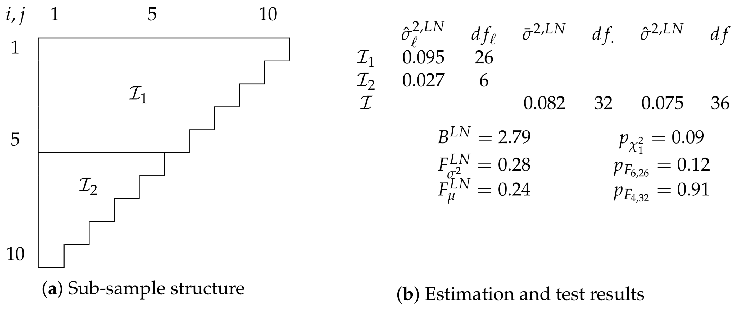
Figure 2 summarizes the results.
Figure 2a shows how we split the data
, a run-off triangle with ten accident and development years. We split into two sub-samples:
contains the first five and
the last five accident years. Choosing this specific structure seems intuitive given
Kuang et al. (
2015) remarks about the location of large residuals.
Given the sub-samples, we specify the unrestricted independent log-normal model
We first consider the hypothesis
for a reduction to
Figure 2b shows the relevant estimates and test results. Since we have just two sub-samples, we can test the hypothesis either with a Bartlett test or an
F-test for common variances. The two test give a rather similar indication. The Bartlett statistic
has a
p-value of 0.09 and the
F-statistic
a two-sided
p-value of 0.12.
If we take the variance test results as an indication not to reject
, we can take
as our primary model and test for
. That is, we test for a reduction to
Based on the F-statistic , we cannot reject this hypothesis with a p-value of 0.91. Thus, we do not find compelling evidence against a reduction to .
Alternatively, we could make use of the information that there is not just a discrepancy between the sub-samples when it comes to residuals, but that those in are larger. With this information, we could alternatively have conducted a one-sided F-test for a one-sided hypothesis . This test yields a p-value of 0.06, a much closer call. Note that we cannot evaluate one-sided hypotheses with a Bartlett test.
5.2. Over-Dispersed Poisson Chain-Ladder
The
Taylor and Ashe (
1983) data in
Table 1 has served many times as an empirical application for over-dispersed Poisson chain-ladder models. Thus, it seems only appropriate to investigate the model specification. We summarize results in
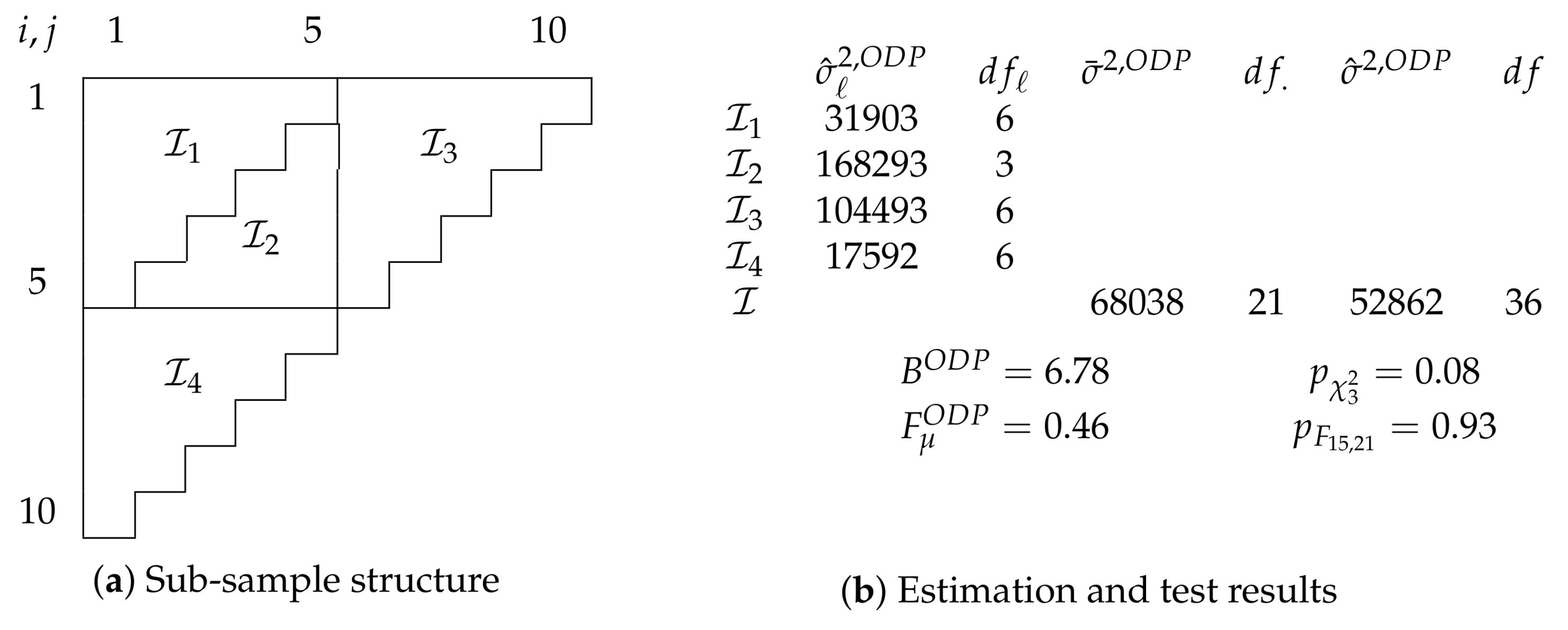
Figure 3.
Figure 3a shows the chosen sub-sample structure. We split the sample after the fifth accident, development, and calendar year into four sub-samples. Unlike in the case of the
Verrall et al. (
2010) data above, we do not have information indicating a specific sub-sample structure. While arbitrary, we find the chosen structure appealing because all sub-samples are run-off triangles themselves and of relatively similar size. Further, we hope that splits after each of the three time-scales increases our chances to find breaks. We point out that the specific sub-sample structure has no effect on the size of the tests if the hypothesis is true.
Figure 3b shows estimates and test results. The unrestricted model is the over-dispersed Poisson model discussed in
Section 4.1 so that
Looking at evidence for varying over-dispersion, we test for with a Bartlett test. While we can see quite a bit of variation in the dispersion estimates, ranging from 17,592 to 168,293, the test does not convincingly reject the hypothesis with a p-value of 0.08. Even though relative deviations from the degree of freedom weighted average 68,038 are less stark, it seems to us that making a decision by eyeballing alone would be difficult in this case.
If the Bartlett test results convince us that a reduction to is sensible, we can test for common linear predictors. Given an F-statistic of = 0.46, we cannot reject this simplification with a p-value of 0.93.
Overall, the target over-dispersed Poisson model for the
Taylor and Ashe (
1983) data survives both misspecification tests at a 5% level for this sub-sample structure. Thus, we may be more confident now to model it with an over-dispersed Poisson chain-ladder model.
We could also opt to repeat the test for other sub-sample structures, adjusting the size to take into account that tests for different sub-sample structures on the same data are generally not independent. For example, retesting for the split into two sub-samples consider above and shown in
Figure 1a. For this structure, a Bartlett test statistic of
= 2.89 yields a
p-value of 0.09 and an
F-test statistic of
= 0.63 a
p-value of 0.64. Further, we can test for a split into three sub-samples after calendar years four and seven, similar to the structure in
Figure 1b. For this structure, we get
= 1.27 with a
p-value of 0.53 and
= 1.84 with a
p-value of 0.11. Controlling the overall size of the thrice repeated sequential tests with a Bonferroni correction, we would reject if any
p-value was below 5%/3 ≈ 0.017. This is not the case so the model survives this battery of tests as well.
5.3. Log-Normal (Extended) Chain-Ladder
As a final empirical application, we look at a run-off triangle first considered by
Barnett and Zehnwirth (
2000). We show this data in
Table A2. These data are known to be modeled best with a predictor with not just accident and development, but also calendar effects. We look at a model with and without calendar effects.
Barnett and Zehnwirth (
2000) and also
Kuang et al. (
2011) consider a log-normal model for this data and we follow them in this choice. As before, we split the data, specify the model, and test for the hypotheses. The results are summarized in
Figure 4.
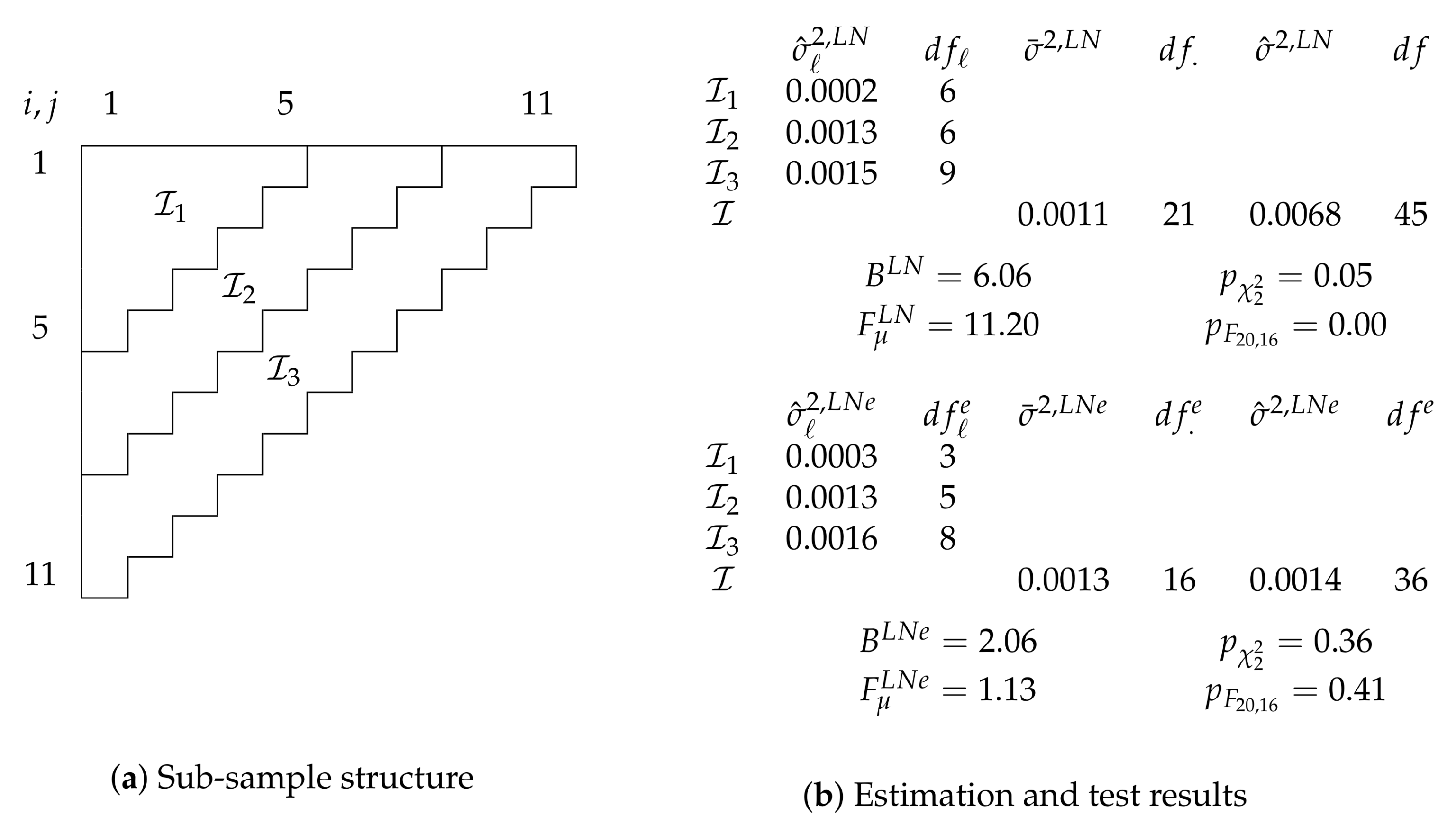
Figure 4a shows the sub-sample structure we choose. Given the apparent need for calendar effects, we aim to maximize power for varying dispersion parameters along the same time dimension and split the run-off triangle, this time with eleven accident and development years, after periods five and eight into three sub-samples.
The top of
Figure 4b shows estimation and test results for a model without calendar effect. This model is given by
A Bartlett test for the hypothesis of common log data variances has a p-value of (just under) 0.05. We may consider this as evidence against . For comparison with the model with calendar effect considered next, we still compute an F-test for the hypothesis . We point out that this test is not strictly a test for common linear-predictors if we are not comfortable to accept as a model. The statistic = 11.20 has a 0.00 p-value so that we reject . Thus, is not well specified.
At the bottom of
Figure 4b we show results for a model with calendar effects
for calendar years
. The model is
The theory for specification tests is not affected by this change and thus still valid. A Bartlett test for in this model yields a p-value of 0.36 so we may feel comfortable to impose common log data variances and take as given. An F-test for common linear predictors leaves us with a p-value of 0.41. Thus, reducing the model to seems sensible. Therefore, we cannot reject the specification of the model with calendar effect.
If we directly compare the two models, we can see that the calendar effect has a substantial impact on the specification tests. While the model with calendar effect seems to be well specified, the model without this effect raises red flags for both a test for common variances and common linear predictors. The test for common linear predictors is much more strongly affected by dropping the calendar effect than the Bartlett test. This indicates that the shift in log data variances is smaller than that in linear predictors.
We look at the shift in linear predictor in two ways. First, we can directly test for for dropping the calendar effects from the well specified . A standard F-test for the hypothesis yields a p-value of 0.00, consistent with the rejection of the model without calendar effects above.
Alternatively, we can test for a reduction from to , corresponding to the hypothesis . This reduction allows for breaks in linear predictors between sub-samples. Interestingly, an F-test cannot reject (p-value 0.92). As an intuition, we recall that the chain-ladder predictor without calendar effects can accommodate a constant trend in calendar years, but not deviations from that trend. Thus, allowing for separate sets of linear predictors on the sub-samples implicitly allows for three different calendar trends. While still less flexible than the model with an effect for each calendar year, this seems to be good enough. Note, however, that the Bartlett flags the reduction from to (but not from to ).
Overall, the analysis suggests that calendar effects are needed in this data set for two reasons for this sub-sample structure: to capture the structure of the linear predictors themselves, and, to a lesser extent, to achieve homogeneous variance across the log data.
We note that for this data, repeating the tests for different sub-samples structures does affect the results. Indeed, considering sub-samples similar to before, the specification of the log-normal extended chain-ladder model is rejected. Specifically, splitting the data into two sub-samples after the fifth accident year, a Bartlett test yields a p-value of 0.017 and an F-test a p-value of 0.004. Considering four sub-samples with splits after the fifth calendar year, the fifth development year and the sixth accident year, the p-value of the Bartlett test is 0.03 and that of the F-test 0.05. Again controlling the size of the repeated tests with a Bonferroni correction, we would reject the null hypothesis if we can find a p-value below about 0.017. This is the case for the F-test and a knife-edge decision for the Bartlett test in the two sub-sample scenario. Thus, for this data we may want to consider a different model or at least be somewhat more skeptical of its results.
6. Simulations
The developed theory begs several questions that we answer in a simulation study. First, we argued that we can sidestep simulating critical values of the Bartlett distribution and instead approximate these by a Bartlett corrected critical value. We show that this works very well. Second, we compute power curves of Bartlett and F-test for common log data variances under several alternatives in a log-normal model to get a better understanding for the tests’ behavior. Third, we show that an asymptotic approximation in an over-dispersed Poisson model resembles the asymptotic distribution closely, both under the null and the considered alternatives. Finally, we derived above that F-tests for common linear predictors in the over-dispersed Poisson model are asymptotically independent of tests for common over-dispersion. We confirm that the size of the former test seems unaffected by conditioning on the results of the latter, even in finite samples.
6.1. Performance of Bartlett test Approximation
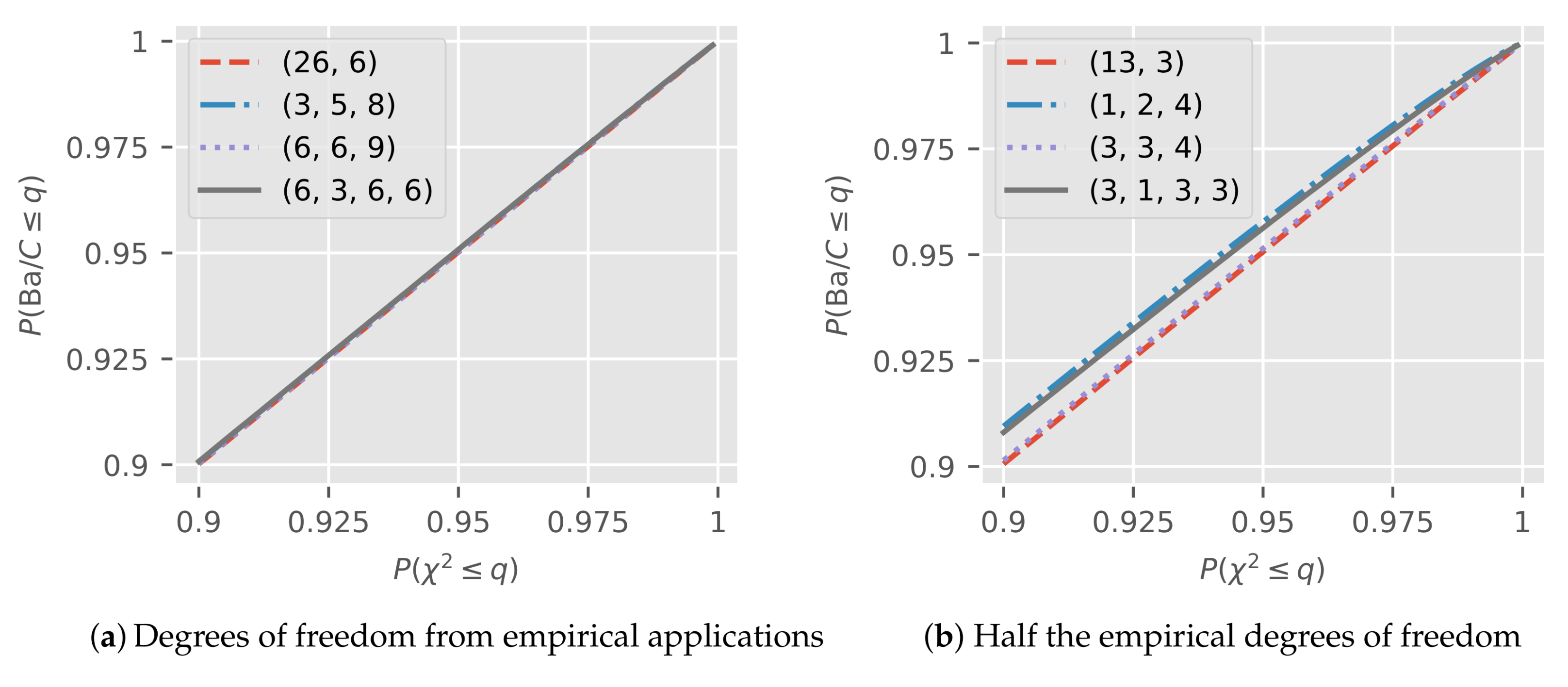
The theory tells us that the distribution of , which is the exact distribution of the Bartlett statistic in the log-normal model, is close to a for large degrees of freedom. We show that the approximation works very well for a range of degrees of freedom.
We draw realizations from the adjusted Bartlett distribution as follows. For , we draw independent distributed with degrees of freedom and compute and . Then, is distributed.
Figure 5a shows the upper 10% probability spectrum of a pp-plot for the adjusted Bartlett distribution
against a
. We show plots for the tuples
,
,
, and
encountered in the empirical applications above. The plots are based on
draws for each tuple. The plots seem indistinguishable from the 45-degree line, even though we zoomed in to the upper 10% of the spectrum.
Figure 5b is constructed in the same way as
Figure 5a, except the degrees of freedom are halved and rounded down. Now, we can see some deviations from the 45-degree line. As expected, we can see convergence to the 45-degree line as the degrees of freedom increase.
In
Table 2, we take a closer look at the approximation at
= 1%, 5%, 10% critical values
of a
specifically. The table shows
, corresponding to the true size of a Bartlett test in a log-normal model if we use the
approximation rather than simulated critical values.
While we can see some differences for some of the halved critical values, we would argue that the approximation for the degree of freedom tuples from the empirical applications is so good that using it is reasonable and should not affect the modeling decision.
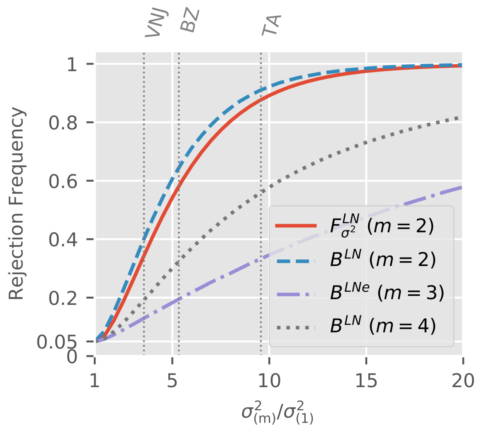
6.2. Rejection Frequencies of Tests for Common Variance in Log-Normal Model
As a supplement to the behavior of the tests for common log data variance under the null hypothesis in the log-normal model given in
Section 3.3, we now also take a look at power. We simulate the three sub-sample structures from the empirical applications and consider rejection frequencies of the tests used in the corresponding applications. We find that the Bartlett and
F-test for common variance have very similar power, at least in this simulation. Further, we see that the power does not necessarily decrease with the number of sub-samples.
For the sub-sample structures from the empirical applications (see
Figure 1), we simulate
. Thus, we simulate for
sub-samples. Before specifying the parameter values, we point out that the distribution of tests in this model depends only on ratios
, the degrees of freedom
, and the number of sub-samples
m. To see this, we first re-write
Now, under , independently. Thus, the distribution of is invariant to common changes in levels of as well as to . Therefore, we can normalize the smallest to unity and set without loss of generality. The distribution of the F-statistic shares these properties.
For each sub-sample scenario, we consider a range of values for the log data variance ratios
. For
sub-samples there is more than one ratio such that we cannot effectively visualize all combinations. We thus consider the following special case. For each sub-sample structure, we the compute the spacing of the estimates from the corresponding empirical application. That is, we order the empirical estimates
and compute the
m spacing-coefficients
. We note that
and
. The spacings
in the empirical examples are
(
Verrall et al. 2010),
(
Barnett and Zehnwirth 2000), and
(
Taylor and Ashe 1983). The log data variance for the
ℓ-th subset is then
To trace out power curves, we vary the largest ratio from one, corresponding to , to twenty in 0.5 increments. As noted above, we can set without loss of generality. For each degree of freedom scenario and for each ratio , we draw sub-samples.
For each draw, we compute the test statistics used in the corresponding empirical application, as in (6) and as in (5). We note that for , we compute only the Bartlett test statistic for the model with calendar effect to make the plot less cluttered. Thus, the degrees of freedom for in the three scenarios are , and . We use critical values for the Bartlett tests.
Figure 6 shows rejection frequencies at 5% critical values.
We can see that all tests have the right size under , that is for . The power of two-sided F-test and Bartlett test in the two sub-sample scenario is very similar with a slight advantage for the Bartlett test. Thus, the choice between the two test may mostly depend on taste. Comparing Bartlett tests across scenarios, we see that the power for sub-samples is larger than that for sub-samples. Thus, fewer sub-samples do not necessarily imply higher power. Intuition comes from the degree of freedom weighting. For sub-samples, if we drop the variance with the smallest degree of freedom the larger two variances are relatively homogeneous. Meanwhile, for sub-samples there is still plenty of variation left among the largest three variances. Thus, since the test attributes more weight to the better estimates with higher degrees of freedom, the scenario with sub-samples is a rather tough case.
We indicated the
ratios we found in the individual empirical applications by vertical lines. We recall that the spacing of intermediate variances is taken from the empirical applications. Therefore, suppose that the empirical estimates are the truth such that
is violated. Then we can read of the power against this scenario directly from the plot. For example, in the application to the
Verrall et al. (
2010) data, the
F-test would have a power of about 35% while the Bartlett test power would be closer to 40%.
6.3. Performance of Over-Dispersed Poisson Model Asymptotics
The theoretical results for the over-dispersed Poisson model are asymptotic, rather than exact as in the log-normal model. We show that an asymptotic approximation works well. Tests for common over-dispersion have the right size under the null. The power under the alternative in finite samples is close to the asymptotic power. Further, F-tests for common linear predictors conditional on non-rejection of over-dispersion tests are very close to F distributed in finite samples.
6.3.1. Rejection Frequencies of Tests for Common Over-Dispersion
We can use the rejection frequencies from the log-normal simulations as a benchmark for those in the over-dispersed Poisson model. To see this we recall that as the overall mean , the over-dispersion estimator in the over-dispersed Poisson model . This matches the exact distribution of in . Thus, asymptotically, the distribution of in and in are identical for identical ratios . The same holds for and .
We simulate for the same three sub-sample structures as in the log-normal simulations. For the simulation design, we set-up an unrestricted model
that satisfies the assumptions in
Section 4.1. For the distribution of the cells we choose compound Poisson-gamma so
where
independent of the i.i.d. gamma distributed
with scale
and shape
. We note that the parametrization for the linear predictors
and the level of the over-dispersion
matters in finite samples. This is in contrast to the log-normal model. The reason is that the finite sample distribution of
in
is generally not
. Thus, for each considered scenario, we set the linear predictors
to the estimates
from the data in the corresponding empirical application. Similarly, we set the smallest over-dispersion
.
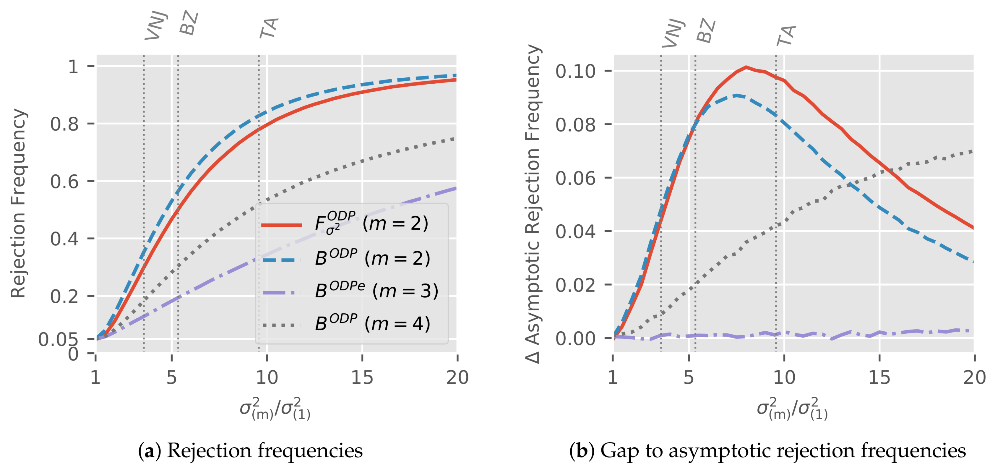
We again vary the ratios from one to twenty, using the exact same spacing from (13) in the log-normal simulations so . The only difference is that now . Therefore, asymptotically, the power for a common is identical in over-dispersed Poisson and log-normal models. We draw sub-samples for each over-dispersion ratio and sub-sample structure.
Figure 7a shows the rejection frequencies at 5% critical values for the four test statistics from the empirical applications as in the log-normal model but now computed based on
.
For
we are under the null; we can see that the rejection frequencies are very close to 5% so the tests have the correct size. Under the alternative where
, the ordering of the rejection frequencies matches that in the log-normal simulations (
Figure 6). Generally, the plot is reassuringly reminiscent of its equivalent in the log-normal simulations.
Figure 7b shows the gap to the asymptotic rejection frequencies that arises in the finite sample simulations. The simulation set-up implies that this is the difference between rejection frequencies in log-normal and over-dispersed Poisson simulations. Thus, the plots shows the impact of the asymptotic approximation in the over-dispersed model. Since the difference under the alternative is positive throughout, the power in the over-dispersed model is lower than in the log-normal model. We next interpret the plots under the alternative in turn for the three sub-sample scenarios.
For
, the power gap of Bartlett and
F-test initially increases with
, hitting
(percentage points)for the
F-test at
, before it decreases. The initial increase relates to the asymptotic theory by
Harnau and Nielsen (
2017) which assumes fixed dispersion parameters. Since we keep
constant, the remaining dispersion parameters grow with the ratio. Thus, we would require larger cell-means to achieve the same asymptotic approximation quality. The later decrease reflects the upper bound of one for the power: even as the asymptotic approximation becomes worse, the difference between dispersion parameters becomes so large that it is easily caught. For
, the power gap is increasing throughout the considered range for
. The intuition for the increase again comes from the asymptotic theory. We do not see a decrease since the power is still quite far from unity, staying below 80% even for the largest maximum to minimum ratio. Meanwhile, for
, the power gap is essentially zero so that the finite sample power matches the asymptotic power. The intuition for this follows because the dispersion to mean ratio is small. As a rough indication, dividing the largest considered dispersion
by the mean over all cells
yields 0.8% for the
Barnett and Zehnwirth (
2000) simulations compared with 70% and 56% for the
Verrall et al. (
2010) and
Taylor and Ashe (
1983) simulations, respectively.
We again indicate the power at the particular alternative generated by taking the estimates in the empirical applications as true values by vertical lines.
Figure 7b shows that for these alternatives, the power for all asymptotic approximations is within
of their asymptotic power.
6.3.2. Independence of Test for Common Linear Predictors
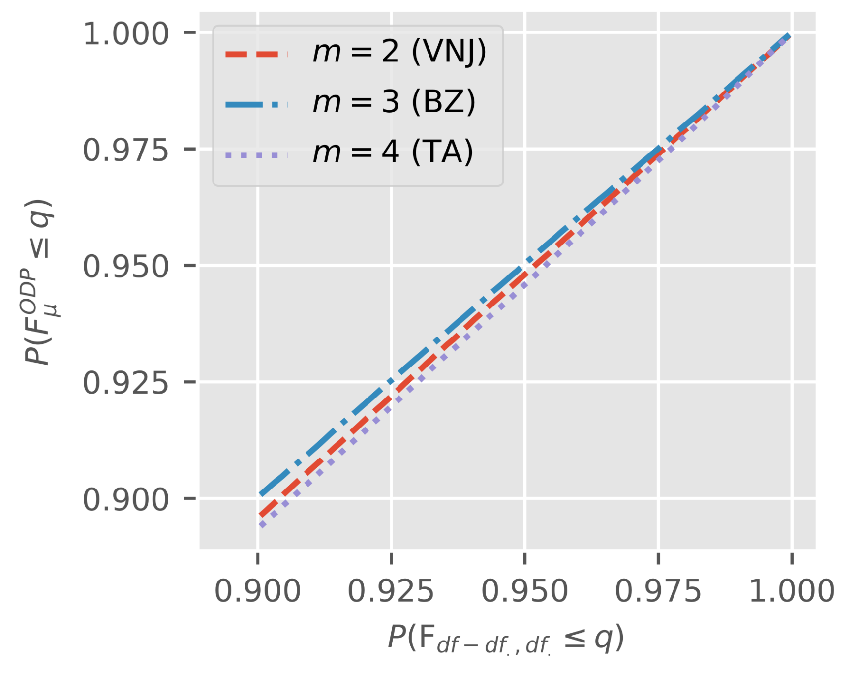
We move on to evaluate the quality of a finite sample approximation to the asymptotic independence in Lemma 1. Specifically, we consider the finite sample distribution of as in (11) given that a tests for common over-dispersion did not reject. Arguably, this is the most interesting case since it matches the natural order of the two specification tests.
We simulate under the null , that is for a model with common linear predictors and over-dispersion . As before, cells are compound Poisson-gamma. We consider three scenarios, setting the parameters to the estimates for in the three empirical examples. We draws 106 triangles per scenario.
For each draw, we compute tests based on the sub-sample structure of the corresponding empirical application. We first conduct a Bartlett test for at 5% critical values. If we do not reject based on this test, we keep the triangle, otherwise we throw it out. Since we simulate under the null hypothesis, we thus keep about 95% of the draws. Only for the draws we keep do we compute the F-statistic for common linear predictors .
Figure 8 shows a pp-plot for the
against
for the triangles that survived Bartlett testing.
To be able to tell a difference from the 45-degree line, we limit our attention to the upper 10% of the probability spectrum since. This is also the most interesting range for testing. Even in this spectrum, each plot is very close to the 45-degree line. Therefore, under , we can be reassured that an F-test for common linear predictors has the correct size in finite samples even if we apply it only conditionally on non-rejection of a test for common over-dispersion.
6.4. Remark
We note that all simulations are for tests that consider the correct sub-sample structure under the alternative. Of course, this does not seem realistic in applications. However, for tests computed on a given sub-sample structure, it appears we would generally be able to choose a true, different, sub-sample structure against which the tests would at best have limited power. For example, say we compute the tests on the two sub-samples with a split after the fifth accident year in
Figure 1a while really there are three sub-samples with an additional split after the fifth development year. Then, we could choose parameterizations for the three true true sub-samples to balance out the variation between the two incorrectly chosen sub-samples, thus minimizing power. Therefore, it seems to us that such simulation results would be almost entirely driven by our chosen parametrization and provide little insight beyond that. We believe the real answer to this problem must come from a theory that is agnostic to the sub-sample structure as discussed below. However, we stress again that the size of the tests under the null hypothesis is not affected by the chosen sub-sample structure.
7. Discussion
Some questions are left open for future research. For example, it is not clear how to best choose the sub-sample structure and the number of sub-samples. Further, the question arises whether we can somehow select between the over-dispersed Poisson and log-normal model. Finally, a misspecification test for independence of the cells would be a useful addition to the modeling toolkit.
So far, we chose the sub-sample structures somewhat arbitrarily if potentially informed by prior knowledge of the data. While the size of the tests under the null is not affected by the sub-sample structure, the power of the tests under the alternative is affected both by the chosen number of sub-samples and their structure. In applications, the expert may consider choosing a range of sub-samples structures and conducting tests for each, adjusting the size based on the number of tests to account for multiple testing as shown in the empirical applications. For future research, it would be useful to derive a theory that is agnostic to the number of sub-samples and their structure while still directly controlling size. It might be fruitful to look for ideas in time-series econometrics which has been concerned with tests for parameter breaks for a long time. In this literature,
Chow (
1960) had proposed a test for parameter breaks that required knowledge of the breakpoint. By now, there are several test available that are agnostic with respect to the number of breaks, related to the number of sub-samples in our problem, and the position of breaks, akin to the sub-sample structure. Examples include Andrews’ test (
Andrews 1993), generalizations of Chow tests (
Nielsen and Whitby 2015), and indicator saturation (
Hendry 1999). However, these tests are designed for data with a single time-scale and results are generally based on long time-series. In contrast, we are confronted with data with three interlinked time-scales and the arrays are often small with a large number of parameters that is growing with the array size. Thus, the known results do not carry over and a it appears that a new theory is needed.
Since we have seen two models in this paper, log-normal and over-dispersed Poisson, a natural question is when we should choose which model. As we have seen, the log-normal model assumes a fixed standard deviation to mean ratio while the over-dispersed Poisson model considers the variance to mean ratio to be fixed. Making use of recent results for generalized log-normal models by
Kuang and Nielsen (
2018), a class of models that includes the log-normal but is more general,
Harnau (
2018) proposes a test to distinguish between (generalized) log-normal and over-dispersed Poisson models based on this discrepancy.
Finally, a misspecification test for the assumption that the cells in the array are independent would be useful. This is an assumption that both the log-normal and the over-dispersed Poisson model impose. In contrast, the “distribution free” model by
Mack (
1993) relaxes this somewhat, assuming independence only across accident years.


