The Exponential Estimate of the Ultimate Ruin Probability for the Non-Homogeneous Renewal Risk Model

Faculty of Mathematics and Informatics, Vilnius University, Naugarduko 24, LT-03225 Vilnius, Lithuania
*
Author to whom correspondence should be addressed.
Risks 2018, 6(1), 20; https://doi.org/10.3390/risks6010020
Submission received: 29 January 2018
/
Revised: 1 March 2018
/
Accepted: 6 March 2018
/
Published: 8 March 2018
Abstract
:In this work, the non-homogeneous risk model is considered. In such a model, claims and inter-arrival times are independent but possibly non-identically distributed. The easily verifiable conditions are found such that the ultimate ruin probability of the model satisfies the exponential estimate for all values of the initial surplus . Algorithms to estimate the positive constant are also presented. In fact, these algorithms are the main contribution of this work. Sharpness of the derived inequalities is illustrated by several numerical examples.
Keywords:
non-homogeneous model; renewal risk model; ruin probability; net profit condition; Lundberg’s inequalityMSC:
91B30; 60E15; 60G501. Introduction
Insurance is a means of protection from random and untoward events, which can lead to significant financial losses. It is a method of risk management, that is used in order to hedge against a contingent loss risk. Risk theory came into being and was developed in order to provide a basis for the existence and significance of the insurance system. One of the most fundamental problems in risk theory is the ruin problem. It analyzes the behavior of a stochastic process, that represents the evolution of the capital of an insurance company. The objective is to estimate the ruin probability, so that the surplus at some time becomes negative. From an insurer’s point of view, the surplus can be defined as “initial surplus + premium income − claim payment”.
The simplest model, which describes the behavior of the insurer’s surplus with respect to time, is the discrete time risk model. It describes insurer’s capital level only in discrete time moments. Although this model is not very applicable in practice, it has been extensively investigated by many authors in theoretical results (see, for instance, Lefèvre and Loisel (2008); Leipus and Šiaulys (2011); Picard and Lefèvre (1997); Seal (1969); Tang (2004b); De Vylder and Goovaerts (1988)).
An extension of the discrete time risk model in the context of values of the insurer’s surplus at an arbitrary time moment is a classical risk model. Its development was begun at the beginning of the twentieth century by Lundberg and Cramér (see Cramér 1930; Cramér 1969; Lundberg 1903; Lundberg 1932; Rolski et al. 1999). They assumed that the special kind of counting process describes the number of appeared claims. In this model, the homogeneous Poisson process describes the number of claims until each time moment because of exponentially and identically distributed inter-arrival times between the consecutive claims. It is difficult to apply such a restriction of the classical risk model for real insurance activities. According to Dickson (2005), this model is a simplification of reality, however, this is a useful model, which can give some insight into the characteristics of an insurance operation.
A more general model is the renewal risk model, which was introduced by Anderson in 1957 (see Andersen 1957; Thorin 1974). In this case, it is supposed that the inter-arrival times between consecutive claims are independent and identically (but not necessarily exponentially) distributed, positive or non-negative (see, for instance, Tang (2004a)) random variables. After such improvement, the new model has become easier to use for real short-term insurance activities. However, from the mathematical point of view, the renewal risk model is more complicated due to the main part of the model being the so-called renewal counting process, whose behavior is quite different from the homogeneous Poisson process.
In the classical risk theory, all models discussed above divert our attention only to the case of homogeneous models. However, it is evident that the non-homogeneous models better reflect the real insurance activities compared to homogeneous models. Therefore, some authors extended the homogeneous renewal risk model into a non-homogeneous one in different ways. Some of them investigated non-homogeneous renewal risk models with independent, identically distributed claims and inter-arrival times, but mutual independence of these two sequences is no longer required (see, for instance, Albrecher and Teugels (2006); Li et al. (2010); Liu et al. (2017b)). Other authors worked with the claim sizes, which have a common distribution function and not necessarily identically distributed inter-arrival times (see Bernackaitė and Šiaulys 2015, 2017; Burnecki and Giuricich 2017; Mao et al. 2017). Other authors dealt with identically distributed claims and inter-arrival times, but there may be some kind of dependence between them (see Chen and Ng 2007; Huang et al. 2017; Constantinescu et al. 2016; Liu and Gao 2016; Li and Sendova 2015; Shen et al. 2016; Yang and Yuen 2016; Yang and Konstantinides 2015; Yang et al. 2014; Wang et al. 2013). Some authors consider models in which claim amounts are divided in several lines by supposing some dependence relations between these lines (see Fu and Ng 2017; Guo et al. 2017; Yang and Yuen 2016). In this work, we consider a non-homogeneous renewal risk model with independent, but not necessarily identically distributed claims and inter-arrival times like in articles by Andrulytė et al. (2015), Kievinaitė and Šiaulys (2018) and Răducan et al. (2015).
We say that the insurer’s surplus varies according to a non-homogeneous renewal risk model, if equation
holds for all with the insurer’s initial surplus , a constant premium rate , a sequence of independent, non-negative and possibly non-identically distributed claim amounts and the renewal counting process , that is generated by the inter-arrival times , which form a sequence of independent, non-negative, not degenerated at zero and possibly non-identically distributed random variables. In addition, sequences and are supposed to be independent.
In the above definition, we say that the constant premium rate and two sequences of random variables and generate the non-homogeneous renewal risk model. If the generating claim amounts are identically distributed and the inter-arrival times are identically distributed, then the non-homogeneous model becomes the homogeneous one.
The central object of the renewal risk model is to investigate the probability that the insurer’s surplus falls below zero at some particular time . In this case, we say that the ruin occurs or, in other words, the insurer becomes unable to pay all the claims. This quantity may be defined as a probability of finite or infinite time ruin probability. Both of these quantities are very important for the insurance company, because the insurer can feel safer when the probability of ruin is low.
The probability of ruin until time moment T is called the finite time ruin probability and is defined by the equality
The infinite time or ultimate ruin probability is defined by equality
The relationship between the finite time ruin probability and the ultimate ruin probability is shown by the formula
By denoting the ruin probability as a function of the initial surplus u, the effect of u for the ruin probability is analyzed. In practice, it is not necessary to know the exact values of the ruin probability. A good estimate of this quantity is sufficient for a risk assessment of an insurer’s business. An exponential bound for the ruin probability is usually called a Lundberg-type inequality. We further give the statement on the upper bound of the ultimate ruin probability in the homogeneous renewal risk model.
Theorem 1.
Let the claims and the inter-arrival times form the homogeneous renewal risk model. Additionally, let the net profit condition hold and for some positive h. Then, there exists a positive H such that
If for some positive R, then we can take in estimate (1).
An exponential upper bound for the ruin probability with constant R is the well-known Lundberg’s inequality. Usually, the number R is unique and called the adjustment coefficient or Lundberg exponent. The Lundberg’s inequality can be proved in different ways. Some of the existing proofs can be found in Asmussen and Albrecher (2010); Embrechts et al. (1997) and Embrechts and Veraverbeke (1982). The most elegant way to prove this inequality is via a martingale approach, which was presented by Gerber (1973). On the other hand, it is sufficient to prove
for all , since we know relationship (see, for instance, Mikosch (2009)). In addition, the Lundberg’s inequality can be proved using the exponential tail bound by Sgibnev (1997) for the random walk supremum and the inequality .
The main purpose of this work is to find easily verifiable conditions so that we could apply a similar Lundberg-type inequality in the non-homogeneous renewal risk model like in the homogeneous one. These assumptions would allow analysis of the model in more realistic cases of insurance. The main results of this paper extend and complement the results of other authors, who have considered the exponential estimate of the ruin probability in the non-homogeneous renewal risk model (see Andrulytė et al. 2015; Kievinaitė and Šiaulys 2018; Castañer et al. 2013; Grandell and Schmidli 2011; Liu et al. 2017a).
The net profit condition is the main condition in Theorem 1. If this condition is not satisfied in the homogeneous renewal risk model, then there is no estimate of the ruin probability, because for each value of the initial surplus . In the case of the non-homogeneous renewal risk model, the probability of ruin depends on the sequence of independent but possibly non-identically distributed random variables . It is neither clear whether the requirement plays the role of the net profit condition in the non-homogeneous renewal risk model, nor whether it is the basis to get exponential upper bound for the probability of ruin. In articles by Andrulytė et al. (2015) and Kievinaitė and Šiaulys (2018), it is supposed that the “net profit condition” holds on average, i.e.,
for sufficiently large . In these works, it is obtained that the above inequality together with other natural requirements imply that , , with some constants and . In our case, we suppose that the “net profit condition” holds on maximum, i.e., for all . The results below show that this stronger condition, together with suitable additional requirements, implies that the probability of ruin can be estimated by the smaller quantity for some positive and for all values of the initial surplus . The main contribution of the paper are the algorithms to estimate this positive parameter .
The non-homogeneous renewal risk model can be rewritten as the random walk generated by a sequence of independent, but not necessarily identically distributed, random variables . Many important results on such a walk in the multi-dimensional space can be found in the book by Menshikov et al. (2016). Our exponential estimates for the ruin probability, derived in this article, complement results of that book.
2. Results
In this section, three assertions are presented on the Lundberg-type inequalities for the ultimate ruin probability in the case of the non-homogeneous renewal risk model. The first assertion below shows that the Lundberg-type estimate for ruin probability holds, if the non-homogeneous model satisfies quite wide requirements. The second theorem supplements Theorem 2. In this theorem, the Lundberg-type inequality, as well as a way to calculate the constant in the exponent, is derived. In order to get that constant all requirements for the model should have expressive forms. The third theorem below is devoted to the sharpest Lundberg-type inequality for the non-homogeneous risk model. However, in general, for this we need to estimate infinitely many “adjustment coefficients”.
In all theorems below, due to traditional definition sequences of random variables, and should be independent. However, from the proofs in Chapter 3, it follows that Theorems 2–4 remain valid when the sequence consists of independent random vectors. If this condition holds, then we can suppose the random variables and to be dependent in an arbitrary way for each index i.
Theorem 2.
Let us consider the non-homogeneous renewal risk model generated by a premium rate , a sequence of independent, non-negative random claims and a sequence of independent, non-negative, not degenerate at zero random inter-arrival times . Let the following three conditions be satisfied:
Then there is a positive constant ϱ such that for all values of the initial surplus .
As stated above, a similar possibility of the exponential estimate was considered by Andrulytė et al. (2015). The more general risk renewal model was investigated in that paper. More precisely, it was supposed that the model satisfies the net profit condition only on average. Naturally, under weaker conditions a rougher estimate of the ruin probability can be obtained.
Theorem 3.
Let us consider the non-homogeneous renewal risk model generated by a premium rate , a sequence of independent, non-negative random claims and a sequence of independent, non-negative, not degenerate at zero random inter-arrival times . In addition, let the following three conditions be satisfied for some constants and :
If, for some ,
then the ultimate ruin probability of the model satisfies exponential upper bound for all values of the initial surplus .
Similar statement on the calculation of an upper exponential bound for the ruin probability was given by Kievinaitė and Šiaulys (2018). Authors of that paper also consider the more general risk renewal model satisfying net profit condition on average. Such a model can have subsequences of random variables with a positive drift. Therefore, the formulas derived there give more conservative upper bounds in comparison to formula of Theorem 3.
Theorem 4.
Let us consider the non-homogeneous renewal risk model generated by a premium rate , a sequence of independent, non-negative random claims and a sequence of independent, non-negative, not degenerate at zero random inter-arrival times . If all conditions of Theorem 2 are satisfied, then there exists an interval such that
for all , and
for all values of the initial surplus .
Theorem 4 has the classical form of Lundberg’s inequality. Inequalities of such a form, for risk renewal models having the special structures, are proved by Castañer et al. (2013); Grandell and Schmidli (2011) and Liu et al. (2017a). It is evident that we need a more explicit expression for to obtain sharp upper exponential bounds for the ruin probability. For example, if for , then the estimate of Theorem 4 implies for .
3. Proofs
This section is devoted to the detailed proofs of all theorems, which are presented in Section 2. Proofs of all these theorems, related with inequality (8) below are provided. If we know that the non-homogeneous renewal risk model satisfies the net profit condition (on maximum) together with two natural related requirements (see Theorem 2), then we derive from (8) the theoretical possibility to have a Lundberg-type exponential bound for the ruin probability. If we know all constants restricting the requirements of the model (see Theorem 3), then, using a slightly different approach, we get from the same inequality an estimate for the parameter of the exponential bound. On the other hand, if the non-homogeneous model satisfies the suitable conditions, then, using the same method as in the proof of Theorem 2, we can obtain the bound of the ruin probability expressed by a supremum of certain exponential moments (see Theorem 4).
Proof of Theorem 2.
Let be the ruin probability within moment of the N-th claim, where and . We have
It is obvious that
Consequently, it is sufficient to prove the inequality
for some positive , for all , for an arbitrary and for an arbitrary collection of different indices .
We will prove this inequality by using induction on N. Let for all .
If , then we derive by the exponential Chebyshev’s inequality that
for all , for all and for an arbitrary .
If and , then we have
In order to estimate the right side of (6), we use the following well-known inequalities:
Using these inequalities, we derive
with and .
We observe that
and
with some constant due to condition (ii) of the theorem.
Thus, using the last estimate we derive that if , then
where is a constant from inequality
Therefore, substituting the obtained estimates into expression (8), we get that
for all and .
Choosing , we derive that
for all .
This estimate and conditions (i), (iii) of the theorem imply that
for some sufficiently small and an arbitrary .
Therefore, according to the inequality (5) we have that
for the same positive , for each and for all .
Now suppose that estimate (4) is correct for , i.e.,
for the above positive coefficient , for all and for an arbitrary collection of different indices .
Proof of Theorem 3.
Let and be probabilities as respectively defined in (3) and (4). For each fixed , is not decreasing with respect to and tends to , when N tends to infinity. In addition,
where indices and .
Hence, for the proof of Theorem 3 it is sufficient to get that
for suitable chosen , for all , for each and for an arbitrary collection of different indices .
We prove this inequality by using induction on N like in the proof of Theorem 2. Let for all as before.
Using inequalities (7), we derive that
for an arbitrary .
It is evident that
and
for an arbitrary positive .
In addition, using theorem’s condition (ii) and inequality we derive that
if .
By substituting the obtained estimates (14), (15), (16) into expression (13), we get that
for all and for an arbitrary index .
Let now with satisfying condition (2). The last estimate implies that
for each .
This together with (5) implies that
for each and for all .
The desired inequality (12) follows from the last two estimates and the induction procedure, which is presented in the proof of Theorem 2 with details. Theorem 3 is proved. ☐
Proof of Theorem 4.
Suppose that for each , as usual. The conditions of the theorem and the estimate (9) imply the existence of an interval such that for each . This is the first assertion of the theorem.
According to estimate (5), we have that
for all , for all and for each .
Using the same proof framework as in Theorem 2, we obtain
for all , and an arbitrary .
Consequently,
for all , . The second assertion of the theorem follows from this and the theorem is proved. ☐
4. Numerical Examples
In this section, we present two examples, which show the applicability of theorems, that are in Section 2. Using the Monte Carlo method, we simulate exact values of ruin probability . We compare these obtained values with upper exponential bounds, which can be derived using the received theoretical results. In Example 1, we investigate the discrete time risk model of five seasons which is a direct generalization of the classical discrete time risk model comprehensively studied by Dickson (2005), see also references therein. As usual, the discrete time risk model describes the insurance business when the insurer calculates surplus at time moments at equal intervals. In Example 2, we consider the non-homogeneous model with complex distributions of claim amounts and inter-arrival times. We show that the corresponding exponential bound can be obtained even for such an unstable model. Naturally, in this case, Theorem 4 should be employed.
Example 1.
Suppose that the non-homogeneous renewal risk model generated by a premium rate , a sequence of degenerated inter-arrival times and a sequence of independent random claims such that for , , and
for .
| 0 | 1 | k | |
- First of all, we find rough estimate of ruin probability according to Theorem 3. After some calculations, we get thatAccording to the above estimates, we obtain that conditions of Theorem 3 hold with parameters and . Substituting the obtained constants into expression (2), we get that the last parameter . Choosing , we get from the assertion of Theorem 3 thatfor all non-negative values of the initial surplus u.The derived estimate is exponential but quite conservative. For instance, it follows from the obtained inequality that , if .
- Now, we find more precise upper bound of ruin probability on the basis of the Theorem 4. All theorem’s conditions hold due to the derived above estimates andFor positive h, we have thatConsequently, for all , and Theorem 4 implies thatfor all values of the initial surplus .The derived estimate is almost four times accurate with respect to the previous one. For instance, it follows from the obtained inequality that , if .
- Finally, we use the Monte Carlo simulations to get approximate values of ruin probability . For this we use the fact that for fixed u and for sufficiently large N. We consider the case when and . For each u, we simulate trajectories of the renewal risk process with N random claims and we calculate how many times on average they fall below zero in order to get values of . According to the obtained values of ruin probability, we get that , even if the initial surplus is especially small, i.e., .
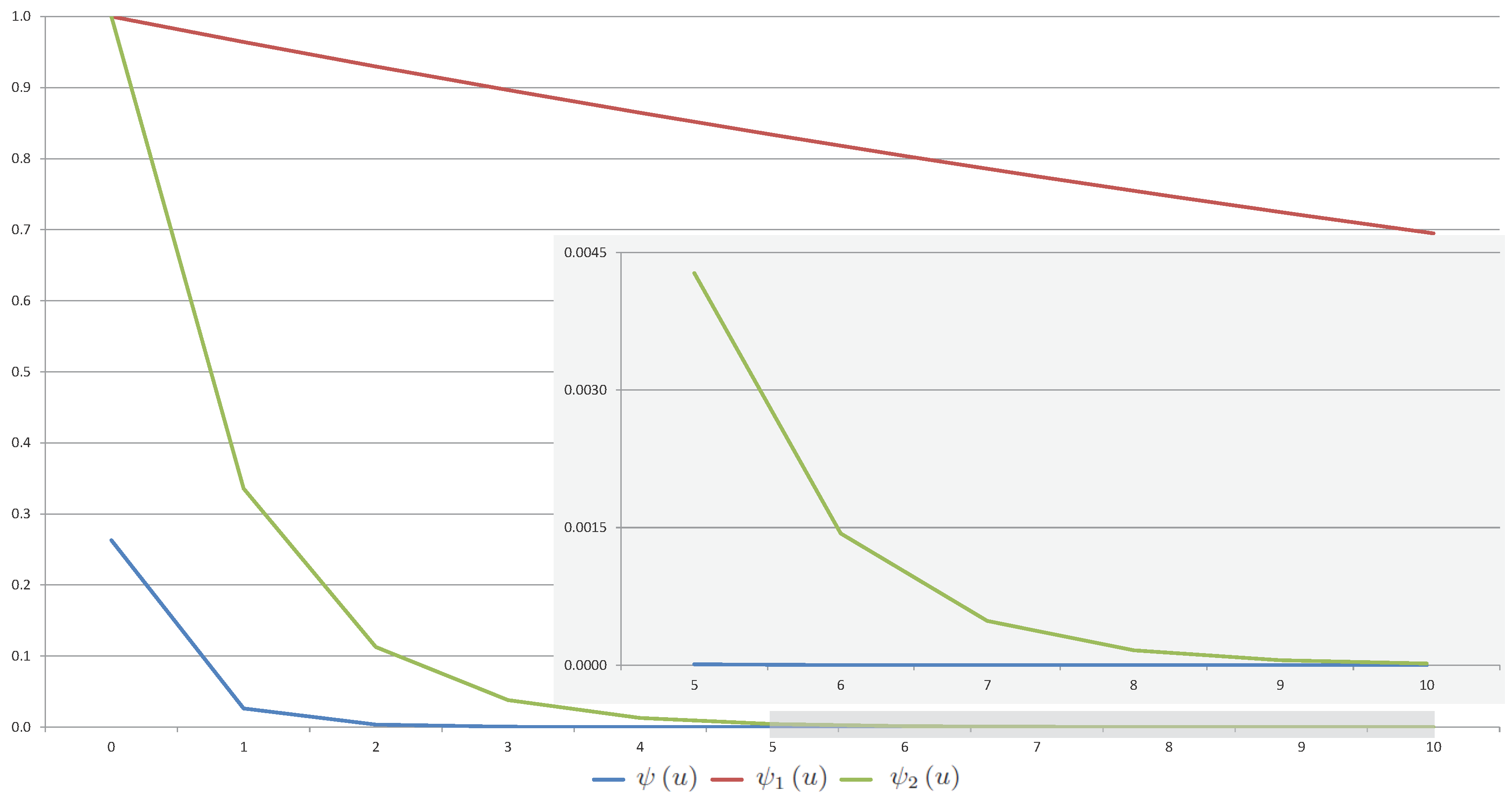
- After the above calculations, for , we can compare approximate values of ruin probability with their conservative estimate and with their sharp estimate . All results are presented in Table 1 and Figure 1. In fact, the conservative exponential upper bound is quite rough, but it is very easy to obtain an expression of this function using Theorem 3. The values of the sharp exponential upper bound are much closer to the simulated values of the ruin probability, however due to Theorem 4, more deeper analysis of the model elements is needed to obtain this bound. Values of , which are obtained by the Monte Carlo method, are sufficiently accurate, but such a procedure takes a lot of time and resources, because we need to generate a lot of process trajectories in order to get these values.
Example 2.
Suppose that the non-homogeneous renewal risk model is generated by a premium rate , a sequence of independent random inter-arrival times and a sequence of independent random claims . The random variable is distributed according to the Gamma law with the shape parameter k and the scale parameter , while the random claim amount is exponentially distributed with parameter , i.e.,
for each . As it is already common, sequences and are supposed to be independent.
The presented model is more complex with respect to the model, which is described in Example 1, because all random variables in sequences and are non-identically distributed. We analyze this example step by step as in the previous one.
- Firstly, we start with the rough estimate of ruin probability, which can be derived using Theorem 3. In the case, we get thatIn addition, we have thatSince random values and are absolutely continuous, so that random value has density, which for all has the following expressionHence, we get thatAccording to the derived estimates, conditions of Theorem 3 hold with such parameters and . Substituting the obtained constants into expression (2), we get that the parameter should be selected from the interval . If , then Theorem 3 implies thatfor all .The derived estimate is extremely conservative. For instance, it follows from the obtained inequality that , if .
- We can use Theorem 4 to obtain the more sharper upper bound for the ruin probability. Conditions of this theorem are satisfied due to the above estimates andIn addition, we have thatfor all .Accordingly, Theorem 4 together with the remark presented after this theorem imply thatfor all .The derived estimate is exponential and almost 30 times more accurate than the previous one. For instance, it follows from the obtained inequality that , if .
- After all these calculations, we again apply the Monte Carlo method in order to get approximate values of ruin probability as in the previous example. We also analyze the same way, while and , and we simulate trajectories of the renewal risk process with N random claims and with N random inter-arrival times for each u. Although this example is sufficiently erratic, on the basis of the received values of ruin probability , we get that , even if the initial surplus is relatively small, i.e., .
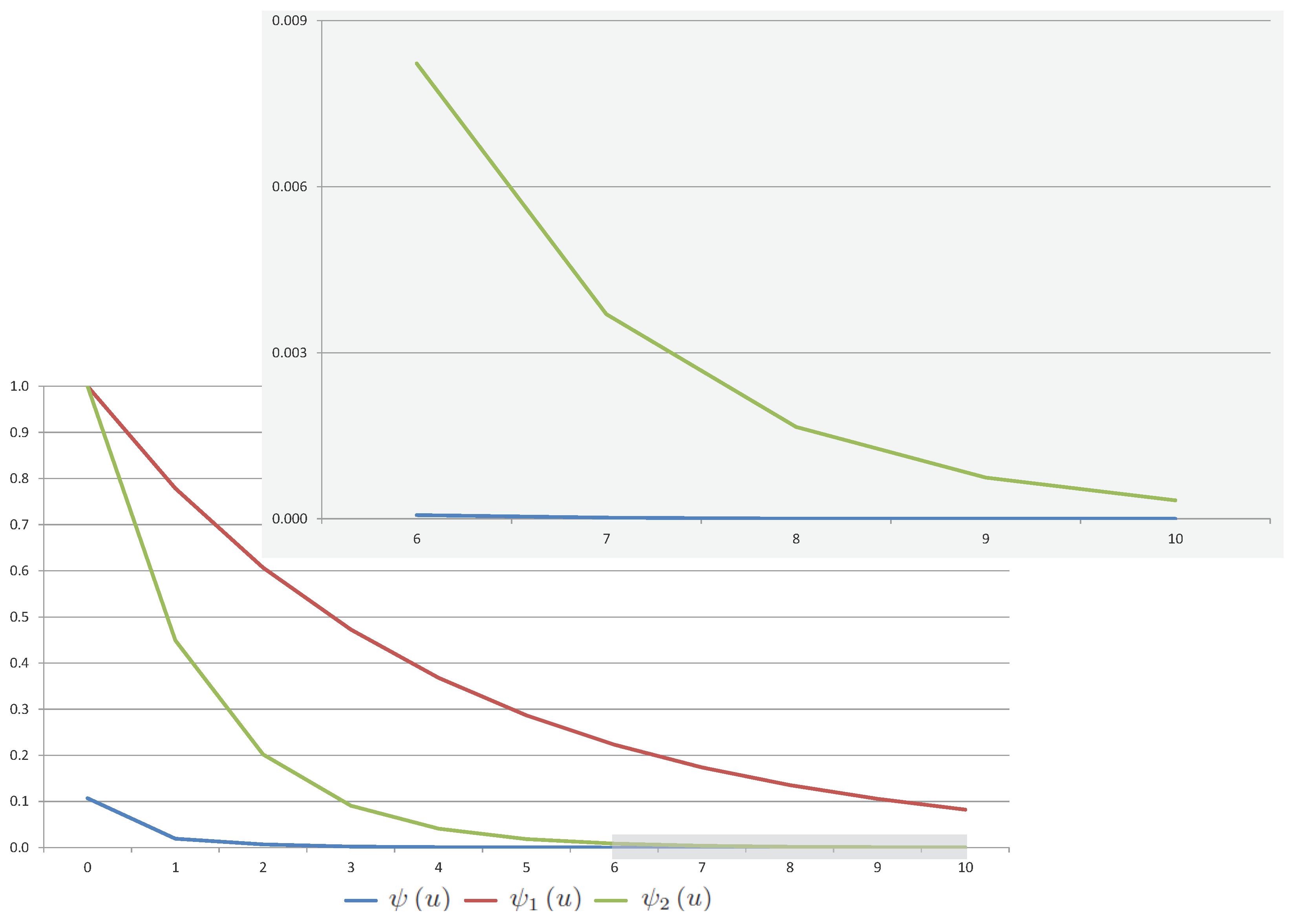
- Ultimately, we can make a comparison of approximate values of ruin probability to their conservative exponential upper bound and to their sharp exponential upper bound for . All results are presented in Table 2 and Figure 2. Actually, the conservative estimate is too rough. The values of sharp estimate are more accurate than . It should be noted that the Monte Carlo method takes even more time in this example than in Example 1, because we need to generate values of two random variables and , which are non-identically distributed for each .
5. Conclusions
Lundberg’s inequality or, in other words, an upper bound for the ultimate ruin probability, plays an important role in the homogeneous models. Although, in recent years, non-homogeneous models are considered in many papers, just a few of them contain exponential estimates of the ruin probability. Therefore, our primary goal is to establish conditions leading to a Lundberg-type inequality for a non-homogeneous renewal risk model, which is comparable to the analogous inequality for the homogeneous case. In this paper, three theorems are proved and two examples demonstrating their applicability are given. Theorem 2 guarantees the existence of some positive constant for an upper bound of the ultimate ruin probability. Theorems 3 and 4 demonstrate how that constant can be calculated. Note that Theorem 3 allows for a fast estimate of ruin probability. However, the large number of constants involved in the process makes it difficult to get an optimal estimate. A sharp exponential estimate can be obtained from Theorem 4. However, in this case, to get an explicit expression of an upper bound is an even more complicated process.
Acknowledgments
The authors are grateful to the anonymous reviewers whose constructive comments have led to serious improvements of the article. The research is supported by a grant No. S-MIP-17-72 from the Research Council of Lithuania.
Author Contributions
Both authors contributed equally to research work.
Conflicts of Interest
The authors declare no conflict of interest.
References
- Albrecher, Hansjörg, and Jef L. Teugels. 2006. Exponential behavior in the presence of dependence in risk theory. Journal of Applied Probability 43: 257–73. [Google Scholar] [CrossRef]
- Andersen, E. Sparre. 1957. On the collective theory of risk in case of contagion between claims. Transactions of the XVth International Congress of Actuaries 2: 219–29. [Google Scholar]
- Andrulytė, Ieva Marija, Emilija Bernackaitė, Dominyka Kievinaitė, and Jonas Šiaulys. 2015. A Lundberg-type inequality for an inhomogeneous renewal risk model. Modern Stochastics: Theory and Applications 2: 173–84. [Google Scholar] [CrossRef]
- Asmussen, Søren, and Hansjörg Albrecher. 2010. Ruin Probabilities. Hackensack: World Scientific. [Google Scholar]
- Bernackaitė, Emilija, and Jonas Šiaulys. 2015. The exponential moment tail of inhomogeneous renewal process. Statistics & Probability Letters 97: 9–15. [Google Scholar]
- Bernackaitė, Emilija, and Jonas Šiaulys. 2017. The finite-time ruin probability for an inhomogeneous renewal risk model. Journal of Industrial and Management Optimization 13: 207–22. [Google Scholar]
- Burnecki, Krzysztof, and Mario Nicoló Giuricich. 2017. Stable weak approximation at work in index-linked catastrophe bond pricing. Risks 5: 64. [Google Scholar] [CrossRef]
- Castañer, Anna, M. Mercè Claramunt, Maude Gathy, Claude Lefèvre, and Maite Mármol. 2013. Ruin problems for a discrete time risk model with non-homogeneous conditions. Scandinavian Actuarial Journal 2013: 83–102. [Google Scholar] [CrossRef]
- Chen, Yiqing, and Kai W. Ng. 2007. The ruin probability of the renewal model with constant interest force and negatively dependent heavy-tailed claims. Insurance: Mathematics and Economics 40: 415–23. [Google Scholar] [CrossRef]
- Constantinescu, Corina, Suhang Dai, Weihong Ni, and Zbigniew Palmowski. 2016. Ruin probabilities with dependence on the number of claims within a fixed time window. Risks 4: 17. [Google Scholar] [CrossRef]
- Cramér, Harald. 1930. On the Mathematical Theory of Risk. Stockholm: Skandia Jubilee Volume. [Google Scholar]
- Cramér, Harald. 1969. Historical review of Filip Lundberg’s works on risk theory. Scandinavian Actuarial Journal 1969: 6–12. [Google Scholar] [CrossRef]
- De Vylder, F. Etienne, and Marc J. Goovaerts. 1988. Recursive calculation of finite-time ruin probabilities. Insurance: Mathematics and Economics 7: 1–7. [Google Scholar] [CrossRef]
- Dickson, David C. M. 2005. Insurance Risk and Ruin. Cambridge: Cambridge University Press. [Google Scholar]
- Embrechts, Paul, Claudia Klüppelberg, and Thomas Mikosch. 1997. Modelling Extremal Events. New York: Springer. [Google Scholar]
- Embrechts, Paul, and Noël Veraverbeke. 1982. Estimates for probability of ruin with special emphasis on the possibility of large claims. Insurance: Mathematics and Economics 1: 55–72. [Google Scholar] [CrossRef]
- Fu, Ke-Ang, and Cheuk Yin Andrew Ng. 2017. Uniform asymptotics for the ruin probabilities of a two-dimensional renewal risk model with dependent claims and risky investments. Statistics & Probability Letters 125: 227–35. [Google Scholar]
- Gerber, Hans U. 1973. Martingales in risk theory. Bulletin Association of Swiss Actuaries 73: 205–16. [Google Scholar]
- Grandell, Jan, and Hanspeter Schmidli. 2011. Ruin probabilities in a diffusion enviroment. Journal of Applied Probability 48A: 39–50. [Google Scholar] [CrossRef]
- Guo, Fenglong, Dingcheng Wang, and Hailiang Yang. 2017. Asymptotic results for ruin probability in a two-dimensional risk model with stochastic investment returns. Journal of Computational and Applied Mathematics 325: 198–221. [Google Scholar] [CrossRef]
- Huang, Xing-Fang, Ting Zhang, Yang Yang, and Tao Jiang. 2017. Ruin probabilities in a dependent discrete-time risk model with gamma-like tailed insurance risks. Risks 5: 14. [Google Scholar] [CrossRef]
- Kievinaitė, Dominyka, and Jonas Šiaulys. 2018. Exponential bounds for the tail probability of the supremum of an inhomogeneous random walk. Modern Stochastics: Theory and Applications. accepted. [Google Scholar]
- Lefèvre, Claude, and Stéphane Loisel. 2008. On finite-time ruin probabilities for classical risk models. Scandinavian Actuarial Journal 2008: 41–60. [Google Scholar] [CrossRef]
- Leipus, Remigijus, and Jonas Šiaulys. 2011. Finite-horizon ruin probability asymptotics in the compound discrete-time risk model. Lithuanian Mathematical Journal 51: 207–19. [Google Scholar] [CrossRef]
- Li, Jinzhu, Qihe Tang, and Rong Wu. 2010. Subexponential tails of discounted aggregate claims in a time-dependent renewal risk model. Advances in Applied Probability 42: 1126–46. [Google Scholar] [CrossRef]
- Li, Zhong, and Kristina P. Sendova. 2015. On a ruin model with both interclaim times and premiums depending on claim sizes. Scandinavian Actuarial Journal 2015: 245–65. [Google Scholar] [CrossRef]
- Liu, Peng, Chunsheng Zhang, and Lanpeng Ji. 2017a. A note on ruin problems in perturbed classical risk models. Statistics & Probability Letters 120: 28–33. [Google Scholar]
- Liu, Rongfei, Dingcheng Wang, and Jiangyan Peng. 2017b. Infinite-time ruin probability of a renewal risk model with exponential Levy process investment and dependent claims and inter-arriwal times. Journal of Industrial and Management Optimization 13: 995–1007. [Google Scholar]
- Liu, Xijun, and Qingwu Gao. 2016. Uniformly asymptotic behavior for the tail probability of discounted aggregate claims in the time-dependent risk model with upper tail assymptotically independent claims. Communications in Statistics—Theory and Methods 45: 5341–54. [Google Scholar] [CrossRef]
- Lundberg, Filip. 1903. Approximerad Framställning av Sannolikehetsfunktionen. Uppsala: Återförsäkring av Kollektivrisker. [Google Scholar]
- Lundberg, Filip. 1932. Some supplementary researches on the collective risk theory. Scandinavian Actuarial Journal 1932: 137–158. [Google Scholar] [CrossRef]
- Mao, Yanzhu, Kaiyong Wang, and Ling Zhu Yue Ren. 2017. Asymptotics for the finite-time ruin probability of a risk model with a general counting process. Japan Journal of Industrial and Applied Mathematics 34: 243–52. [Google Scholar] [CrossRef]
- Menshikov, Mikhail, Serguei Popov, and Andrew Wade. 2016. Non-homogeneous Random Walks. Cambridge: Cambridge University Press. [Google Scholar]
- Mikosch, Thomas. 2009. Non-life Insurance Mathematics. New York: Springer. [Google Scholar]
- Picard, Philippe, and Claude Lefèvre. 1997. The probability of ruin in finite time with discrete claim size distribution. Scandinavian Actuarial Journal 1997: 58–69. [Google Scholar] [CrossRef]
- Rolski, Tomasz, Hanspeter Schmidli, Volker Schmidt, and Jozef Teugels. 1999. Stochastic Processes for Insurance and Finance. Hoboken: John Wiley & Sons Ltd. [Google Scholar]
- Răducan, Anisoara Maria, Raluca Vernic, and Gheorghita Zbaganu. 2015. Recursive calculation of ruin probabilities at or before claim instants for non-iddentically distributed claims. ASTIN Bulletin 45: 421–443. [Google Scholar] [CrossRef]
- Seal, Hilary L. 1969. Stochastic Theory of a Risk Business. New York: Wiley. [Google Scholar]
- Sgibnev, Mikhail. 1997. Submultiplicative moments of the supremum of a random walk with negative drift. Statistics & Probability Letters 32: 377–383. [Google Scholar]
- Shen, Xinmei, Menghao Xu, and Ebenezer Fiifi Emire Atta Mills. 2016. Precise large deviation results for sums of sub-exponential claims in a size-dependent renewal risk model. Statistics & Probability Letters 114: 6–13. [Google Scholar]
- Tang, Qihe. 2004a. Asymptotics for the finite time ruin probability in the renewal model with consistent variation. Stochastic Models 20: 281–97. [Google Scholar] [CrossRef]
- Tang, Qihe. 2004b. The ruin probability of a discrete time risk model under constant interest rate with heavy tails. Scandinavian Actuarial Journal 2004: 229–40. [Google Scholar] [CrossRef]
- Thorin, Olof. 1974. Some comments on the Sparre Andersen model in the risk theory. ASTIN Bulletin 81: 104–25. [Google Scholar] [CrossRef]
- Wang, Kaiyong, Yuebao Wang, and Qingwu Gao. 2013. Uniform asymptotics for the finite-time ruin probability of a dependent risk model with a constant interest rate. Methodology and Computing in Applied Probability 15: 109–24. [Google Scholar] [CrossRef]
- Yang, Yang, and Dimitrios G. Konstantinides. 2015. Asymptotics fot ruin probabilities in a discrete-time risk model with dependent financial and insurance risks. Scandinavian Actuarial Journal 2015: 641–59. [Google Scholar] [CrossRef]
- Yang, Yang, Kaiyong Wang, and Dimitrios G. Konstantinides. 2014. Uniform asymptotics for discounted aggregate claims in dependent risk models. Journal of Applied Probability 51: 669–84. [Google Scholar] [CrossRef]
- Yang, Yang, and Kam C. Yuen. 2016. Finite-time and infinite-time ruin probabilities in a two-dimensional delayed renewal risk model with Sarmanov dependent claims. Journal of Mathematical Analysis and Applications 442: 600–26. [Google Scholar] [CrossRef]
Figure 1.
Ruin probability for model of Example 1.

Figure 2.
Ruin probability for model of Example 2.

Table 1.
Values and estimates of ruin probability for model of Example 1.
| u | |||
|---|---|---|---|
| 0 | 0.1069843 | 1.0000000 | 1.0000000 |
| 1 | 0.0192021 | 0.7866279 | 0.3906278 |
| 2 | 0.0068947 | 0.6187834 | 0.1525901 |
| 3 | 0.0019112 | 0.4867523 | 0.0596059 |
| 4 | 0.0006655 | 0.3828929 | 0.0232837 |
| 5 | 0.0002378 | 0.3011942 | 0.0090953 |
| 6 | 0.0000675 | 0.2369278 | 0.0035529 |
| 7 | 0.0000217 | 0.1863740 | 0.0013878 |
| 8 | 0.0000060 | 0.1466070 | 0.0005421 |
| 9 | 0.0000014 | 0.1153251 | 0.0002118 |
| 10 | 0.0000006 | 0.0907180 | 0.0000827 |
Table 2.
Values and estimates of ruin probability for model of Example 2.
| u | |||
|---|---|---|---|
| 0 | 0.2628618 | 1.0000000 | 1.0000000 |
| 1 | 0.0262527 | 0.9642545 | 0.3359110 |
| 2 | 0.0035110 | 0.9297868 | 0.1128362 |
| 3 | 0.0005077 | 0.8965511 | 0.0379029 |
| 4 | 0.0000739 | 0.8645034 | 0.0127320 |
| 5 | 0.0000102 | 0.8336013 | 0.0042768 |
| 6 | 0.0000015 | 0.8038039 | 0.0014366 |
| 7 | 0.0000001 | 0.7750715 | 0.0004826 |
| 8 | 0.0000000 | 0.7473662 | 0.0001621 |
| 9 | 0.0000000 | 0.7206512 | 0.0000545 |
| 10 | 0.0000000 | 0.6948912 | 0.0000183 |
© 2018 by the authors. Licensee MDPI, Basel, Switzerland. This article is an open access article distributed under the terms and conditions of the Creative Commons Attribution (CC BY) license (http://creativecommons.org/licenses/by/4.0/).
Share and Cite
MDPI and ACS Style
Kizinevič, E.; Šiaulys, J. The Exponential Estimate of the Ultimate Ruin Probability for the Non-Homogeneous Renewal Risk Model. Risks 2018, 6, 20. https://doi.org/10.3390/risks6010020
AMA Style
Kizinevič E, Šiaulys J. The Exponential Estimate of the Ultimate Ruin Probability for the Non-Homogeneous Renewal Risk Model. Risks. 2018; 6(1):20. https://doi.org/10.3390/risks6010020
Chicago/Turabian StyleKizinevič, Edita, and Jonas Šiaulys. 2018. "The Exponential Estimate of the Ultimate Ruin Probability for the Non-Homogeneous Renewal Risk Model" Risks 6, no. 1: 20. https://doi.org/10.3390/risks6010020
Note that from the first issue of 2016, this journal uses article numbers instead of page numbers. See further details here.