A Generalized Measure for the Optimal Portfolio Selection Problem and its Explicit Solution

1
Actuarial Research Center, Department of Statistics, University of Haifa, Mount Carmel, 3498838 Haifa, Israel
2
Department of Economics and Business Management, Ariel University, Ariel 40700, Israel
*
Author to whom correspondence should be addressed.
Risks 2018, 6(1), 19; https://doi.org/10.3390/risks6010019
Submission received: 4 January 2018
/
Revised: 20 February 2018
/
Accepted: 26 February 2018
/
Published: 6 March 2018
Abstract
:In this paper, we offer a novel class of utility functions applied to optimal portfolio selection. This class incorporates as special cases important measures such as the mean-variance, Sharpe ratio, mean-standard deviation and others. We provide an explicit solution to the problem of optimal portfolio selection based on this class. Furthermore, we show that each measure in this class generally reduces to the efficient frontier that coincides or belongs to the classical mean-variance efficient frontier. In addition, a condition is provided for the existence of the a one-to-one correspondence between the parameter of this class of utility functions and the trade-off parameter in the mean-variance utility function. This correspondence essentially provides insight into the choice of this parameter. We illustrate our results by taking a portfolio of stocks from National Association of Securities Dealers Automated Quotation (NASDAQ).
1. Introduction
The portfolio selection problem is of both theoretical and of practical interest (Castellano and Cerqueti 2014; Li and Hoi 2014; Shen et al. 2014; Fletcher 2015; Fulga 2016; Ray and Jenamani 2016). The pioneering work of Markowitz (1952) (see Elton and Gruber. 1987; Steinbach 2001) on optimal portfolio selection (OPS) introduced the classical mean variance (MV) approach
which has been studied extensively in the financial literature (Landsman and Valdez 2003; Li and Hoi 2014; Bera et al. 2015; Graham et al. 2015; Qin 2015; Markowitz 2014). Here is the portfolio return, and are vectors of weights and excess returns, respectively, and where is vector of n ones. , where is the vector of expected returns and where is the covariance matrix of the vector of portfolio excess returns.Let us notice that the mean-variance model is the balanced difference between the expectation of returns, which measures an average asset profit, and the variance of returns, which measures the associated risk. Maximization of is motivated, therefore, by maximization of average asset profit and minimization of asset risk. Let us also notice that in the case when short selling is possible, the mean-variance OPS problem has an analytic explicit-form solution, because it reduces to a classical quadratic programming problem.
Another key approach in the OPS theory is the maximization of the Sharpe ratio (see, for instance, Sharpe 1998), which was introduced in Sharpe (1966), and has the form
where is the risk free rate. Here we have a ratio between expectation of returns and their standard deviation. Again, the maximization of the Sharpe ratio is motivated by maximization of expected profit and minimization of risk. We observe that there is no analytic solution to this maximization problem even for the situation when short selling is permitted.
In this paper, we offer a novel utility measure, which generalizes both the mean-variance, Sharpe measures and many other celebrated risk measures, and represents a much more flexible measure for incorporating and ,
Here and are differentiable functions, where is a monotonic increasing function, i.e., is a positive convex or concave function, and is defined on and is positive on .
We found an analytical explicit-form solution of the optimization of the general functional subject to a system of affine equality constraints, when short selling is permitted. The solution takes the following explicit form
where both and have explicit closed-forms and they do not depend on the functionals and which means that these vectors are the same for different OPS models (e.g., the MV and the Sharpe ratio models), while the parameter depends on the models that are used.
2. Main Results
The generalized measure we introduce is based on the maximization of (3) subject to the linear constraints
where is rectangular matrix of full rank, is some vector and is a vector-column of m zeros. The motivation of such a system of linear constraints arises from models, such as the MV, where the linear constraint ascertains that the sum of the weights of the portfolio is equal to one, with positive and negative values corresponding to long and short positions, respectively. More elaborate systems of constraints associated with optimal portfolio selection can be found in Best and Grauer (1990); Landsman (2008b), and in Landsman and Makov (2016). For example, in the case where and B is of dimension and is equal to
Equation (5) represents the case when the expected return of a sub-portfolio of size j (the first j returns) is equal to and the expected return of a remaining sub-portfolio of size (the remaining returns) is equal to
We show that the solution of the maximization of (3) subject to (5), is taking an explicit form, which coincides with the solution of the mean-variance problem (16), where the trade-off parameter is and is a solution of an algebraic equation to be presented later.
Before we formulate the main theorem, we begin by introducing certain notations and partitions, which will be helpful in the sequel. Consider the natural partitions of vector where and and consider the respective partitions of and , where are vectors of n ones and zeros, respectively. In a similar way, let us partition the matrix
and matrix
where matrices and are of dimensions and respectively. As matrix B is full rank, suppose, without loss of generality, that matrix is non singular.
Furthermore, we define and matrices
and matrix
Notice that as is positive definite, Q is also positive definite (see Landsman 2008a).
We note that function must satisfies the following condition:
(C) The function is strictly convex on for any numbers and r such that
This condition is essentially weaker than a condition of convexity of For example, is concave but condition (C) still holds.
Theorem 1.
Suppose that and If the following equation with respect to
has a positive solution this solution is unique and the problem of maximization
subject to (5) coincides with the solution of the mean-variance optimal problem, where the trade-off parameter λ takes the value
In other words the solution to (11) is given by
Here
and
The proof of the Theorem is given in the Appendix A.
This Theorem essentially generalizes Theorem 1 of Landsman and Makov (2016), where a special case was considered when . Notice that in Landsman and Makov (2016) vector was presented in a less convenient form than that of (A19).
Theorem 1 may have the following economic interpretation: it expresses the competition between the minimum variance portfolio and vector these vectors appear in the classical mean variance portfolio and do not depend on the choice of the utility function and tuning parameter which reflects by investor’s preference. From expression of vector (A19), immediately follows that
Then, for the special case, when , matrix and we have and the vector can be interpreted as a self-financing portfolio in the sense that long-positions are financed by corresponding short positions (see, for instance, Panjer and Boyle (1998), sct. 8.2.1). This case is considered in more details below, in Remark 1.
We now state a property related to the efficient frontier of the class of utility measures generated by (3). First of all we notice that for our utility function (3)
These inequalities are very natural and important. They say that utility function is increased with respect to and decreased with respect to
Corollary 1.
The proof of the Corollary is given in the Appendix A.
Remark 1.
In the special case when matrix and we can conclude that
which conform with Panjer and Boyle (1998, (8.2.7)–(8.2.9)). See also (Steinbach 2001, Theorem 1.4). From (A22) follows that elements of the efficient frontier are
The orthogonality property (A20) for this case was proved by Best and Best and Grauer (1990).
2.1. Optimal Portfolios for Special Cases
The investigated generalized measure, includes, as special cases, key measures employed in risk management.
We now show some special cases of the generalized measure
Special case 2: Generalized Sharpe ratio (GSR). We introduce a generalized Sharpe ratio
which is a special case of (3), for which and and found an analytic solution of the corresponding optimization problem for The economic justification for introducing this utility function can be explained by investor’s wish to allow faster decrease in the utility when the variance increases. In this section, we show that as the investors are more risk-averse they should consider larger value of the power function parameter, so is subjective for each investor. The parameter can be interpreted as a new risk aversion parameter, which was absent in the classical Sharpe ratio. This risk measure is much more flexible than the classical Sharpe ratio for which In Section 2.1.4 we explain this in more details.
Special case 3: Mean Variance (MV). In this case, and and the goal function (3) takes the form
Special case 4: Mean Standard Deviation (MSD). In the case and (3) has the form
This functional arises in risk management and actuarial theory. For instance, the value at risk and the expected shortfall takes the form (17) for returns having elliptical distribution (see, for example, Landsman and Valdez (2003)).
2.1.1. Optimal Portfolio Selection With MV Measure
This case was implicitly considered in the proof of Theorem 1. Recall that for MV and , and the functions and take the forms Therefore, Equation (10) simply reduces to
It is clear that is positive and unique, and the point of maximum is (12) with Clearly, this optimal solution is only meaningful if is specified. Notice that the MV measure can be also computed explicitly from the main Theorem of Landsman and Makov (2016), but, the solution in Landsman and Makov (2016) is much more complex in its form than Theorem 1. This proposed solution well conforms with Panjer and Boyle (1998, (8.2.7)–(8.2.9)).
2.1.2. Optimal Portfolio Selection With MSD
As was discussed in the introduction, for the MSD utility function, and and the main functional reduces to the form
which has a form of a combination of linear functional and a square root of a quadratic functional. The optimal problem with this functional was considered in details in Landsmana (2008a, 2008b). Here we only show how the solution of this problem can be obtained from Theorem 1.
We note that the functions and have the form
and Equation (10), which reduces to
has the positive solution,
iff
Now, substituting into (12), we finally get the maximization solution which conforms with Theorem 1 in Landsman (2008b). Applying Theorem 1 we can say that the optimal portfolio coincides with mean-variance portfolio when the trade off parameter is
Note that although the optimal solution can be derived, in principle, from the mean-variance utility function, the choice of remains a guess, unless calculated ( using the main theorem of this paper.
2.1.3. Optimal Portfolio Selection With Sharpe Ratio
Recall that the Sharpe ratio functional has the form
It is clear that for the solution of the maximization problem it is enough to consider Then and . Consequently functions and simply have the form
Thus Equation (10) reduces to algebraic equation of the first degree and the unique solution is
Now since it is sufficient to determine that iff
the solution of (18) is positive and then we obtain the explicit maximum solution which has the form given in (12).
Hitherto, an optimal portfolio selection for the Sharpe ratio utility function has been unavailable. We establish that the optimal solution is a special case of the mean-variance utility function, where, using (18), can now be calculated to be
2.1.4. Optimal Portfolio With Generalized Sharpe Ratio
The functional of the GSR was introduced previously, as follows:
In this functional, where is a power function. Recall and Now we consider the case where (the case was considered in the previous subsection). Then functions and take the form
and Equation (10) reduces to a quadratic equation with respect to w
where Notice that (20) has the unique positive solution.
and when the maximum solution takes the form of (12).
We now return to the economic interpretation of this functional, comparing it with Sharpe ratio. In fact, returning to the arguments given after Theorem 1 we obtain that
For the speed of decrease of the generalized Sharpe ratio in is higher than that of decrease of the Sharpe ratio
As for the efficient frontier, we conclude from (21) that the efficient frontier corresponding to the generalized and classical Sharpe ratios belongs to the efficient frontier corresponding to the mean-variance model (See proof of Corollary 1), with the following set showing the relation between the MV risk aversion parameter, , and the generalized Sharpe ratio risk aversion parameter, ,
Applying Theorem 1 we can say that the optimal portfolio coincides with mean-variance portfolio when the trade-off parameter is
The following Figure shows the relation between the and As we can see from Figure 1, increased almost proportionally when increases.
Note that acknowledging the fact that the optimal solution corresponds to a solution derived from the mean-variance utility function is not enough since the value of the trade of remains unknown. The result provided here allows us to calculate its value.
3. Numerical Illustrations
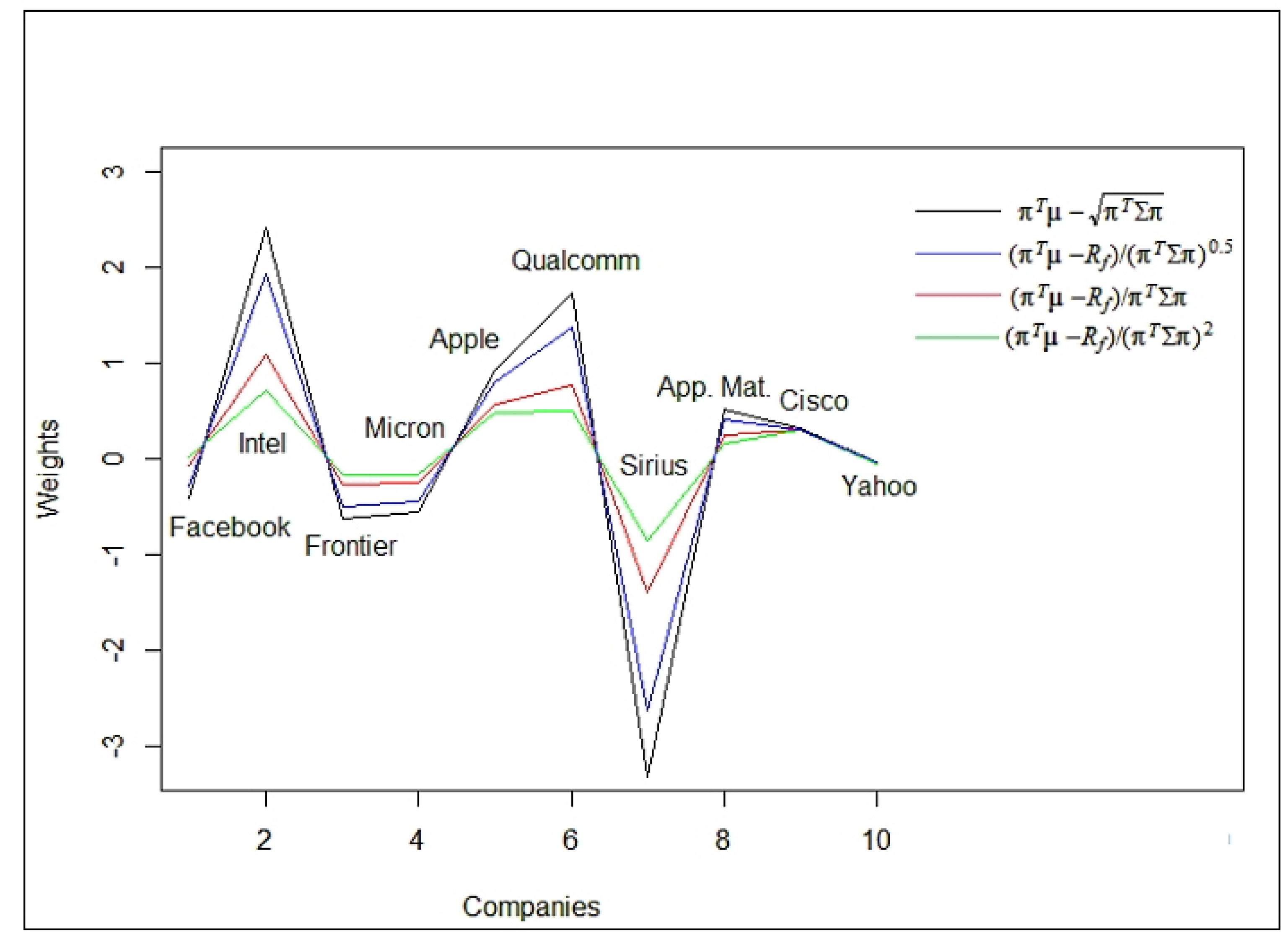
We illustrate the results of the OPS problem for the mean standard deviation utility function and for special cases of the generalized Sharpe ratio
with and free rate for a portfolio of 10 stocks from NASDAQ: Facebook, Intel, Frontier, Micron, Apple, Qualcomm, Sirius, Applied Materials, Cisco and Yahoo, for a three month period of time, from 4 January 15 to 7 January 15—daily returns (For the data, see http://www.nasdaq.com/). Here is the vector of expected returns and is the covariance matrix or returns presented in Table 1 and Table 2, respectively. Furthermore, we assume the traditional linear constraint
Then, using formula (24) we can calculate trade off parameters and then obtain the vectors of solutions, for each model, are given in Table 3.
In the following Figure we present the spectrum of optimal portfolios, given in Table 3.
From Figure 2 it is evident that the amplitude of the weights decreases with increasing values of This well conforms with the graph of presented in Figure 1. As a result it can be observed that the portfolio become more robust when increases. This agrees with the expression of portfolio variance, given in the second formula of (A21), associated with the risk of the portfolio. According to Figure 2, the stocks: Intel, Apple, Qualcomm, App. Mat. and Cisco should be invested in a long position, while the other stocks should be invested in a short position. Furthermore, all of the models are in agreement that the stocks with the largest impact on the portfolio are Intel and Sirius. Table 3, presents the solutions for the different models: MSD, SR and GSR, and together with the graphical illustration (Figure 2) show that all of the mean-variance-based risk measures share the same patterns in terms of higher/lower gains, so the main difference between them is the amplitude.
This numerical illustration shows that investors with a more risk-averse character should consider larger values of than the Sharpe ratio measure. Therefore, the flexibility of the generalized Sharpe ratio is governed by the different values of the subjective parameter corresponding to the level of risk aversion. The generalized Sharpe ratio shows how to implement, naturally, a risk aversion parameter into the framework of the standard Sharpe ratio (2).
4. Conclusions
In this paper, we suggested a novel generalized optimal portfolio selection utility measure which incorporates many popular portfolio selection utility measures as special cases. We further provided an explicit solution to this new utility measure, thus reestablishing existing optimal solutions to portfolio selection and offered closed-form solutions to optimal portfolio selections based on new utility measures which hitherto have not been investigated. We note that while the optimal solution for each of these utility functions can be obtained using the mean-variance utility function, the corresponding is simply unavailable without the methodology presented here. Furthermore, we demonstrated our results using a portfolio consisting ten stocks from NASDAQ in a period of three months and analyzed the results for the mean standard deviation utility function and for the generalized Sharpe ratio.
Acknowledgments
We would like to thank the anonymous referees for their useful comments. This research was supported by the Israel Science Foundation (grant No. 1686/17). The authors also wish to thank the Israel Zimmerman Foundation for the Study of Banking and Finance for financial support.
Author Contributions
The authors contribute equally to this article.
Conflicts of Interest
The authors declare no conflict of interest.
Appendix A. Proofs
Proof of Theorem 1. We first note that since is a convex or concave function, is also a convex or concave function. We further define vector
then, by (5) and (6) it follows that
and straightforwardly
Then the objective function
is a function of variables and the problem reduces to the problem of finding the unconditional maximum
Denoting a vector of derivatives with the following notation
we clearly seek, taking into account (8) and (9), that
Using (8), it is clear that this system of equations can be rewritten in the form
and we denote the solution of (A4) as . In Landsman (2008b) it was shown that as a solution of the quadratic programming problem
Then from (A2) we can represent as a partition
As vector is a point of minimum of quadratic functional , from (A3) it follows immediately that is the solution of the following equation
We will now seek in the form , where is dimensional vector. Then, taking into account (A5), we straightforwardly obtain from (A4),
We represent a matrix as follows:
where is the first row of and consists of the remaining rows of As matrix Q is positive definite, is also positive definite, so there exists a raw r of matrix such that Suppose, without loss of generalization, that Then from (A6) follows the system of equations
where is the first element of vector and is the vector of the last elements of After dividing the last equations of (A8) by its first equation we immediately get that
where
and and take the form (A7). Taking into account (7), (A3) and (A5), we simplify the first equation of (A8) for element as follows
In Landsman (2008a) (eq. 29) it was shown that
which we substitute into (A11) to obtain the one-dimensional equation
From (A13) and from the positivity of and it follows that
should satisfy the following equation
Furthermore, notice that
and taking into account (A5), Equation (A14) is straightforwardly reduced to Equation (10).
Now, since the ratio functional
is the ratio of a convex or concave function and a convex function, our problem is in the field of fractional programming as described in Schaible and Ibaraki (1983). Therefore, since in the theory of fractional programming is known that a local maximum is global and unique, so does our solution of the maximization problem. Recall that is a unique positive solution of Equation (A14). Taking into account (A2), we finally conclude from (A16) that the maximizing vector of weights has the form
where the vector has the following partition
Now let us return to the original maximization problem (11) subject to (5). We have shown that the unique solution of this problem can be written in the form (A17), where neither nor depend on the functional but both depend only on the covariance matrix matrix B and vectors and
Consider the special case of functional when and In this case, using (8) and (9), the functions and simply take the forms
and therefore, Equation (10) reduces to
Note that this optimization problem takes the form
From the solution of the well known quadratic programming problem (see, for example, Luenberger (1984), chp. 14.1, eq. (9)) we can immediately conclude that
Proof of Corollary 1. We show that the random vectors and are orthogonal in the sense that
In fact,
Now let us notice that any specific members of utility (3) would contain the risk parameter, say that reflects to trade-off between expected return and risk, and there is one-to-one map between the set of possible meanings of this parameter, and subset of the positive part of real line, If some utility has no such parameter explicitly we say that contains only one value. For classical mean-variance portfolio and subset If , the corresponding efficient portfolio belongs to that given for classical efficient portfolio.
References
- Bera, Samaresh, Praveen Gupta, and Sudip Misra. 2015. D2S: Dynamic demand scheduling in smart grid using optimal portfolio selection strategy. IEEE Transactions on Smart Grid 6: 1434–42. [Google Scholar] [CrossRef]
- Best, Michael J., and Robert R. Grauer. 1990. The efficient set mathematics when mean-variance problems are subject to general linear constraints. Journal of Economics and Business 42: 105–20. [Google Scholar] [CrossRef]
- Castellano, Rosella, and Roy Cerqueti. 2014. Mean–Variance portfolio selection in presence of infrequently traded stocks. European Journal of Operational Research 234: 442–49. [Google Scholar] [CrossRef]
- Elton, Edwin J., and Martin J. Gruber. 1987. Modern Portfolio Theory and Investment Analysis. New York: Wiley. [Google Scholar]
- Fletcher, Jonathan. 2015. Exploring the benefits of using stock characteristics in optimal portfolio strategies. The European Journal of Finance 23: 1–19. [Google Scholar] [CrossRef] [Green Version]
- Fulga, Cristinca. 2016. Portfolio optimization under loss aversion. European Journal of Operational Research 251: 310–22. [Google Scholar] [CrossRef]
- Graham, John R., Campbell R. Harvey, and Manju Puri. 2015. Capital allocation and delegation of decision-making authority within firms. Journal of Financial Economics 115: 449–70. [Google Scholar] [CrossRef]
- Landsman, Zinoviy, and Emiliano A. Valdez. 2003. Tail conditional expectations for elliptical distributions. North American Actuarial Journal 7: 55–71. [Google Scholar] [CrossRef]
- Landsman, Zinoviy. 2008a. Minimization of the root of a quadratic functional under an affine equality constraint. Journal of Computational and Applied Mathematics 216: 319–27. [Google Scholar] [CrossRef]
- Landsman, Zinoviy. 2008b. Minimization of the root of a quadratic functional under a system of affine equality constraints with application to portfolio management. Journal of Computational and Applied Mathematics 220: 739–48. [Google Scholar] [CrossRef]
- Landsman, Zinoviy, and Udi Makov. 2016. Minimization of a function of a quadratic functional with application to optimal portfolio selection. Journal of Optimization Theory and Application 170: 308–22. [Google Scholar] [CrossRef]
- Li, Bin, and Steven C. H. Hoi. 2014. Online portfolio selection: A survey. ACM Computing Surveys (CSUR) 46: 35. [Google Scholar] [CrossRef]
- Luenberger, David G. 1984. Linear and Nonlinear Programming. Boston: Addison-Wesley. [Google Scholar]
- Markowitz, Harry. 2014. Mean–variance approximations to expected utility. European Journal of Operational Research 234: 346–55. [Google Scholar] [CrossRef]
- Panjer, Harry H., and Phelim. P. Boyle, eds. 1998. Financial economics: With Applications to Investments, Insurance, and Pensions. Schaumburg: Society of Actuaries. [Google Scholar]
- Qin, Zhongfeng. 2015. Mean-variance model for portfolio optimization problem in the simultaneous presence of random and uncertain returns. European Journal of Operational Research 245: 480–88. [Google Scholar] [CrossRef]
- Ray, Pritee, and Mamata Jenamani. 2016. Mean-variance analysis of sourcing decision under disruption risk. European Journal of Operational Research 250: 679–89. [Google Scholar] [CrossRef]
- Schaible, Siegfried, and Toshidide Ibaraki. 1983. Fractional programming. European Journal of Operational Research 12: 325–38. [Google Scholar] [CrossRef]
- Sharpe, William F. 1966. Mutual fund performance. The Journal of Business 39: 119–38. [Google Scholar] [CrossRef]
- Sharpe, William F. 1998. The Sharpe Ratio. Streetwise-The Best of the Journal of Portfolio Management. Princeton: Princeton University Press, pp. 169–85. [Google Scholar]
- Shen, Yang, Xin Zhang, and Tak Kuen Siu. 2014. Mean–variance portfolio selection under a constant elasticity of variance model. Operations Research Letters 42: 337–42. [Google Scholar] [CrossRef]
- Steinbach, Marc C. 2001. Markowitz Revisted: Mean-Variance models in financial portfolio analysis. SIAM Review 43: 31–85. [Google Scholar] [CrossRef]
Figure 1.
The relations between and
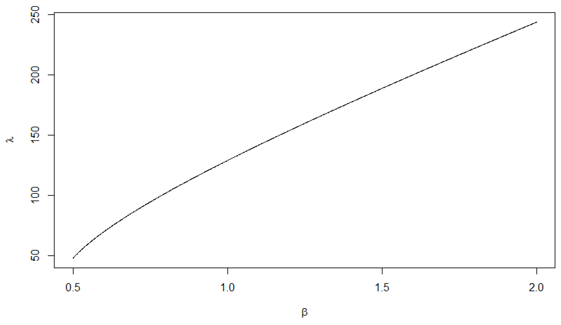
Figure 2.
Optimal portfolios for Mean standard deviation (MSD) and generalized Sharpe ratio, utility functions.
Figure 2.
Optimal portfolios for Mean standard deviation (MSD) and generalized Sharpe ratio, utility functions.

Table 1.
Expected returns.
| Stock | Intel | Frontier | Micron | Apple | |
|---|---|---|---|---|---|
| Mean | 0.000868097 | −0.000608624 | −0.006684089 | −0.006902419 | −6.1631 × 10 |
| Stock | Qualcomm | Sirius | App. Mat. | Cisco | Yahoo |
| Mean | 0.001046047 | 0.000763278 | 0.002049615 | −2.57636 × 10 | 0.001925747 |
Table 2.
Covariance matrix of the returns.
| Intel | Frontier | Micron | Apple | ||
| 0.000175 | 0.000038 | 0.000054 | 0.000063 | −0.000014 | |
| Intel | 0.000038 | 0.000174 | 0.000075 | 0.000213 | −0.000014 |
| Frontier | 0.000054 | 0.000075 | 0.000685 | 0.000031 | −0.000001 |
| Micron | 0.000063 | 0.000213 | 0.000031 | 0.001031 | 0.000048 |
| Apple | −0.000014 | −0.000014 | −0.000001 | 0.000048 | 0.000124 |
| Qualcomm | Sirius | App. Mat. | Cisco | Yahoo | |
| 0.000029 | −0.000015 | −0.000019 | 0.000006 | 0.000010 | |
| Intel | 0.000030 | 0.000086 | 0.000024 | 0.000028 | 0.000047 |
| Frontier | 0.000084 | −0.000014 | 0.000071 | 0.000050 | 0.000095 |
| Micron | 0.000027 | 0.000023 | 0.000050 | −0.000002 | 0.000047 |
| Apple | −0.000002 | 0.000012 | 0.000015 | −0.000010 | 0.000046 |
| Qualcomm | Sirius | App. Mat. | Cisco | Yahoo | |
| Qualcomm | 0.000108 | 0.000054 | 0.000038 | 0.000054 | 0.000075 |
| Sirius XM | 0.000054 | 0.000097 | 0.000049 | 0.000044 | 0.000060 |
| App. Mat. | 0.000038 | 0.000049 | 0.000235 | 0.000046 | 0.000086 |
| Cisco | 0.000054 | 0.000044 | 0.000046 | 0.000084 | 0.000037 |
| Yahoo | 0.000075 | 0.000060 | 0.000086 | 0.000037 | 0.000316 |
Table 3.
The solutions for different models: Mean standard deviation (MSD), Sharpe ratio (SR) and generalized SR.
Table 3.
The solutions for different models: Mean standard deviation (MSD), Sharpe ratio (SR) and generalized SR.
| Utility Function | ||||||
| 61.78 | −0.282 | 1.938 | −0.496 | −0.432 | 0.809 | |
| 47.6 | −0.402 | 2.418 | −0.627 | −0.542 | 0.937 | |
| 128.8 | −0.071 | 1.094 | −0.264 | −0.238 | 0.584 | |
| 243.7 | 0.019 | 0.727 | −0.163 | −0.154 | 0.486 | |
| Utility Function | ||||||
| 1.382 | −2.613 | 0.419 | 0.314 | −0.0391 | ||
| 1.731 | −3.313 | 0.516 | 0.319 | −0.0377 | ||
| 0.766 | −1.382 | 0.247 | 0.305 | −0.041 | ||
| 0.499 | −0.847 | 0.173 | 0.301 | −0.042 |
© 2018 by the authors. Licensee MDPI, Basel, Switzerland. This article is an open access article distributed under the terms and conditions of the Creative Commons Attribution (CC BY) license (http://creativecommons.org/licenses/by/4.0/).
Share and Cite
MDPI and ACS Style
Landsman, Z.; Makov, U.; Shushi, T. A Generalized Measure for the Optimal Portfolio Selection Problem and its Explicit Solution. Risks 2018, 6, 19. https://doi.org/10.3390/risks6010019
AMA Style
Landsman Z, Makov U, Shushi T. A Generalized Measure for the Optimal Portfolio Selection Problem and its Explicit Solution. Risks. 2018; 6(1):19. https://doi.org/10.3390/risks6010019
Chicago/Turabian StyleLandsman, Zinoviy, Udi Makov, and Tomer Shushi. 2018. "A Generalized Measure for the Optimal Portfolio Selection Problem and its Explicit Solution" Risks 6, no. 1: 19. https://doi.org/10.3390/risks6010019
Note that from the first issue of 2016, this journal uses article numbers instead of page numbers. See further details here.