Article

Multivariate Frequency-Severity Regression Models in Insurance

1
School of Business, University of Wisconsin-Madison, 975 University Avenue, Madison, WI 53706, USA
2
Department of Statistics, University of Wisconsin-Madison, 1300 University Avenue, Madison, WI 53706, USA
*
Author to whom correspondence should be addressed.
Submission received: 16 November 2015 / Accepted: 15 February 2016 / Published: 25 February 2016

Abstract

:
In insurance and related industries including healthcare, it is common to have several outcome measures that the analyst wishes to understand using explanatory variables. For example, in automobile insurance, an accident may result in payments for damage to one’s own vehicle, damage to another party’s vehicle, or personal injury. It is also common to be interested in the frequency of accidents in addition to the severity of the claim amounts. This paper synthesizes and extends the literature on multivariate frequency-severity regression modeling with a focus on insurance industry applications. Regression models for understanding the distribution of each outcome continue to be developed yet there now exists a solid body of literature for the marginal outcomes. This paper contributes to this body of literature by focusing on the use of a copula for modeling the dependence among these outcomes; a major advantage of this tool is that it preserves the body of work established for marginal models. We illustrate this approach using data from the Wisconsin Local Government Property Insurance Fund. This fund offers insurance protection for (i) property; (ii) motor vehicle; and (iii) contractors’ equipment claims. In addition to several claim types and frequency-severity components, outcomes can be further categorized by time and space, requiring complex dependency modeling. We find significant dependencies for these data; specifically, we find that dependencies among lines are stronger than the dependencies between the frequency and average severity within each line.

1. Introduction and Motivation

Many insurance data sets feature information about how often claims arise, the frequency, in addition to the claim size, the severity. Observable responses can include:
  • N, the number of claims (events),
  • y k , k = 1 , . . . , N , the amount of each claim (loss), and
  • S = y 1 + + y N , the aggregate claim amount.
By convention, the set { y j } is empty when N = 0 .
Importance of Modeling Frequency. The aggregate claim amount S is the key element for an insurer’s balance sheet, as it represents the amount of money paid on claims. So, why do insurance companies regularly track the frequency of claims as well as the claim amounts? As in an earlier review [1], we can segment these reasons into four categories: (i) features of contracts; (ii) policyholder behavior and risk mitigation; (iii) databases that insurers maintain; and (iv) regulatory requirements.
  • Contractually, it is common for insurers to impose deductibles and policy limits on a per occurrence and on a per contract basis. Knowing only the aggregate claim amount for each policy limits any insights one can get into the impact of these contract features.
  • Covariates that help explain insurance outcomes can differ dramatically between frequency and severity. For example, in healthcare, the decision to utilize healthcare by individuals (the frequency) is related primarily to personal characteristics whereas the cost per user (the severity) may be more related to characteristics of the healthcare provider (such as the physician). Covariates may also be used to represent risk mitigation activities whose impact varies by frequency and severity. For example, in fire insurance, lightning rods help to prevent an accident (frequency) whereas fire extinguishers help to reduce the impact of damage (severity).
  • Many insurers keep data files that suggest developing separate frequency and severity models. For example, insurers maintain a “policyholder” file that is established when a policy is written. A separate file, often known as the “claims” file, records details of the claim against the insurer, including the amount. These separate databases facilitate separate modeling of frequency and severity.
  • Insurance is a closely monitored industry sector. Regulators routinely require the reporting of claims numbers as well as amounts. Moreover, insurers often utilize different administrative systems for handling small, frequently occurring, reimbursable losses, e.g., prescription drugs, versus rare occurrence, high impact events, e.g., inland marine. Every insurance claim means that the insurer incurs additional expenses suggesting that claims frequency is an important determinant of expenses.
Importance of Including Covariates. In this work, we assume that the interest is in the joint modeling of frequency and severity of claims. In actuarial science, there is a long history of studying frequency, severity and the aggregate claim for homogeneous portfolios; that is, identically and independently distributed realizations of random variables. See any introductory actuarial text, such as [2], for an introduction to this rich literature.
In contrast, the focus of this review is to assume that explanatory variables (covariates, predictors) are available to the analyst. Historically, this additional information has been available from a policyholder’s application form, where various characteristics of the policyholder were supplied to the insurer. For example, in motor vehicle insurance, classic rating variables include the age and sex of the driver, type of the vehicle, region in which the vehicle was driven, and so forth. The current industry trend is towards taking advantage of “big data”, with attempts being made to capture additional information about policyholders not available from traditional underwriting sources. An important example is the inclusion of personal credit scores, developed and used in the industry to assess the quality of personal loans, that turn out to also be important predictors of motor vehicle claims experience. Moreover, many insurers are now experimenting with global positioning systems combined with wireless communication to yield real-time policyholder usage data and much more. Through such systems, they gather micro data such as the time of day that the car is driven, sudden changes in acceleration, and so forth. This foray into detailed information is known as “telematics”. See, for example, [3] for further discussion.
Importance of Multivariate Modeling. To summarize reasons for examining insurance outcomes on a multivariate basis, we utilize an earlier review in [4]. In that paper, frequencies were restricted to binary outcomes, corresponding to a claim or no claim, known as “two-part” modeling. In contrast, this paper describes more general frequency modeling, although the motivation for examining multivariate outcomes are similar. Analysts and managers gain useful insights by studying the joint behavior of insurance risks, i.e., a multivariate approach:
  • For some products, insurers must track payments separately by component to meet contractual obligations. For example, in motor vehicle coverage, deductibles and limits depend on the coverage type, e.g., bodily injury, damage to one’s own vehicle, or damage to another party; is natural for the insurer to track claims by coverage type.
  • For other products, there may be no contractual reasons to decompose an obligation by components and yet the insurer does so to help better understand the overall risk. For example, many insurers interested in pricing homeowners insurance are now decomposing the risk by “peril”, or cause of loss. Homeowners is typically sold as an all-risk policy, which covers all causes of loss except those specifically excluded. By decomposing losses into homogenous categories of risk, actuaries seek to get a better understanding of the determinants of each component, resulting in a better overall predictor of losses.
  • It is natural to follow the experience of a policyholder over time, resulting in a vector of observations for each policyholder. This special case of multivariate analysis is known as “panel data”, see, for example, [5].
  • In the same fashion, policy experience can be organized through other hierarchies. For example, it is common to organize experience geographically and analyze spatial relationships.
  • Multivariate models in insurance need not be restricted to only insurance losses. For example, a study of term and whole life insurance ownership is in [6]. As an example in customer retention, both [7,8] advocate for putting the customer at the center of the analysis, meaning that we need to think about the several products that a customer owns simultaneously.
An insurer has a collection of multivariate risks and the interest is managing the distribution of outcomes. Typically, insurers have a collection of tools that can then be used for portfolio management including deductibles, coinsurance, policy limits, renewal underwriting, and reinsurance arrangements. Although pricing of risks can often focus on the mean, with allowances for expenses, profit, and “risk loadings”, understanding capital requirements and firm solvency requires understanding of the portfolio distribution. For this purpose, it is important to treat risks as multivariate in order to get an accurate picture of their dependencies.
Dependence and Contagion. We have seen in the above discussion that dependencies arise naturally when modeling insurance data. As a first approximation, we typically think about risks in a portfolio as being independent from one another and rely upon risk pooling to diversify portfolio risk. However, in some cases, risks share common elements such as an epidemic in a population, a natural disaster such as a hurricane that affects many policyholders simultaneously, or an interest rate environment shared by policies with investment elements. These common (pandemic) elements, often known as “contagion”, induce dependencies that can affect a portfolio’s distribution significantly.
Thus, one approach is to model risks as univariate outcomes but to incorporate dependencies through unobserved “latent” risk factors that are common to risks within a portfolio. This approach is viable in some applications of interest. However, one can also incorporate contagion effects into a more general multivariate approach that we adopt this view in this paper. We will also consider situations where data are available to identify models and so we will be able to use the data to guide our decisions when formulating dependence models.
Modeling dependencies is important for many reasons. These include:
  • Dependencies may impact the statistical significance of parameter estimates.
  • When we examine the distribution of one variable conditional on another, dependencies are important.
  • For prediction, the degree of dependency affects the degree of reliability of our predictions.
  • Insurers want to construct products that do not expose them to extreme variation. They want to understand the distribution of a product that has many identifiable components; to understand the distribution of the overall product, one strategy is to describe the distribution of each product and a relationship among the distributions.
A recent review paper [3] provides additional discussion.
Plan for the Paper. The following is a plan to introduce readers further to the topic. Section 2 gives a brief overview of univariate models, that is, regression models with a single outcome for a response. This section sets the tone and notation for the rest of the paper. Section 3 provides an overview of multivariate modeling, focusing on the “copula” regression approach described here. This section discusses continuous, discrete, and mixed (Tweedie) outcomes. For our regression applications, the focus is mainly on a family of copulas known as “elliptical”, because of their flexibility of modeling pairwise dependence and wide usages in multivariate analysis. Section 3 also summarizes a modeling strategy for the empirical approach of copula regression.
Section 4 reviews other recent work on multivariate frequency-severity model and describes the benefits of diversification, particularly important in an insurance context. To illustrate our ideas and approach, Section 5 and Section 6 provide our analysis using data from the Wisconsin Local Government Property Insurance Fund. Section 7 concludes with a few closing remarks.

2. Univariate Foundations

For notation, define N for the random number of claims, S for the aggregate claim amount, and S ¯ = S / N for the average claim amount (defined to be 0 when N = 0 ). To model these outcomes, we use a collection of covariates x , some of which may be useful for frequency modeling whereas others will be useful for severity modeling. The dependent variables N , S , and S ¯ as well as covariates x vary by the risk i = 1 , , n . For each risk, we also are interested in multivariate outcomes indexed by j = 1 , , p . So, for example, N i = ( N i 1 , , N i p ) represents the vector of p claim outcomes from the ith risk.
This section summarizes modeling approaches for a single outcome ( p = 1 ). A more detailed review can be found in [1].

2.1. Frequency-Severity

For modeling the joint outcome ( N , S ) (or equivalently, ( N , S ¯ ) ), it is customary to first condition on the frequency and then modeling the severity. Suppressing the { i } subscript, we decompose the distribution of the dependent variables as:
f ( N , S ) = f ( N ) × f ( S | N ) joint = frequency × conditional severity,
where f ( N , S ) denotes the joint distribution of ( N , S ) . Through this decomposition, we do not require independence of the frequency and severity components.
There are many ways to model dependence when considering the joint distribution f ( N , S ) in Equation (1). For example, one may use a latent variable that affects both frequency N and loss amounts S, thus inducing a positive association. Copulas are another tool used regularly by actuaries to model non-linear associations and will be described in subsequent Section 4. The conditional probability framework is a natural method of allowing for potential dependencies and provides a good starting platform for empirical work.

2.2. Modeling Frequency Using GLMs

It has become routine for actuarial analysts to model the frequency N i based on covariates x i using generalized linear models, GLMs, cf., [9]. For binary outcomes, logit and probit forms are most commonly used, cf., [10]. For count outcomes, one begins with a Poisson or negative binomial distribution. Moreover, to handle the excessive number of zeros relative to that implied by these distributions, analysts routinely examine zero-inflated models, as described in [11].
A strength of GLMs relative to other non-linear models is that one can express the mean as a simple function of linear combinations of the covariates. In insurance, it is common to use a “logarithmic link” for this function and so express the mean as μ i = E N i = exp ( x i β ) , where β is a vector of parameters associated with the covariates. This function is used because it yields desirable parameter interpretations, seems to fit data reasonably well, and ties well with other approaches traditionally used in actuarial ratemaking applications [12].
It is also common to identify one of the covariates as an “exposure” that is used to calibrate the size of a potential outcome variable. In frequency modeling, the mean is assumed to vary proportionally with E i , for exposure. To incorporate exposures, we specify one of the explanatory variables to be ln E i and restrict the corresponding regression coefficient to be 1; this term is known as an offset. With this convention, we have
ln μ i = ln E i + x i β μ i E i = exp ( x i β ) .
Since there are inflated numbers of 0 s and 1 s in our data, a "zero-one-inflated" model is introduced. As an extension of the zero-inflated method, a zero-one-inflated model employs two generating processes. The first process is governed by a multinomial distribution that generates structural zeros and ones. The second process is governed by a Poisson or negative binomial distribution that generates counts, some of which may be zero or one.
Denote the latent variable in the first process as I i , i = 1 , , n , which follows a multinomial distribution with possible values 0, 1 and 2 with corresponding probabilities π 0 , i , π 1 , i , π 2 , i = 1 - π 0 , i - π 1 , i . Here, N i is frequency.
N i 0 I i = 0 1 I i = 1 P i I i = 2 .
Here, P i may be a Poisson or negative binomial distribution. With this, the probability mass function of N i is
f N , i ( n ) = π 0 , i I { n = 0 } + π 1 , i I { n = 1 } + π 2 , i P i ( n ) .
A logit specification is used to parameterize the probabilities for the latent variable I i . Denote the covariates associated with I i as z i . A logit specification is used to parameterize the probabilities for the latent variable I i . Using level 2 as a reference, the specification is
l o g π j , i π 2 , i = z i γ j , j = 0 , 1 .
Correspondingly,
π j , i = exp ( z i γ j ) 1 + exp ( z i γ j ) + exp ( z i γ j ) , j = 0 , 1 .
π 2 , i = 1 - π 0 , i - π 1 , i
Maximum likelihood estimation is used to fit the parameters.

2.3. Modeling Severity

Modeling Severity Using GLMs. For insurance analysts, one strength of the GLM approach is that the same set of routines can be used for continuous as well as discrete outcomes. For severities, it is common to use a gamma or inverse Gaussian distribution, often with a logarithmic link (primarily for parameter interpretability).
One strength of the linear exponential family that forms the basis of GLMs is that a sample average of outcomes comes from the same distribution as the outcomes. Specifically, suppose that we have m independent variables from the same distribution with location parameter θ and scale parameter ϕ . Then, the sample average comes from the same distributional family with location parameter θ and scale parameter ϕ / m . This result is helpful as insurance analysts regularly face grouped data as well as individual data. For example, [1] provides a demonstration of this basic property.
To illustrate, in the aggregate claims model, if individual losses have a gamma distribution with mean μ i and scale parameter ϕ , then, conditional on observing N i losses, the average aggregate loss S ¯ i has a gamma distribution with mean μ i and scale parameter ϕ / N i .
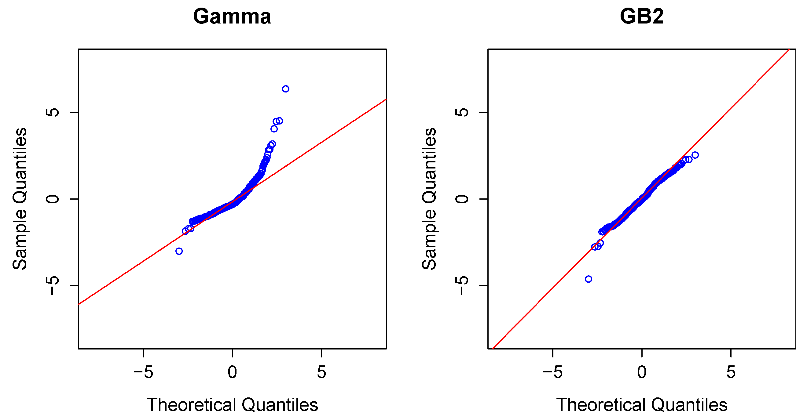
Modeling Severity Using GB2. The GLM is the workhorse for industry analysts interested in analyzing the severity of claims. Naturally, because of the importance of claims severity, a number of alternative approaches have been explored, cf., [13] for an introduction. In this review, we focus on a specific alternative, using a distribution family known as the “generalized beta of the second kind”, or GB2, for short.
A random variable with a GB2 distribution can be written as
e μ G 1 G 2 σ = C 1 e μ F σ = e μ Z 1 - Z σ ,
where the constant C 1 = ( α 1 / α 2 ) σ , G 1 and G 2 are independent gamma random variables with scale parameter 1 and shape parameters α 1 and α 2 , respectively. Further, the random variable F has an F-distribution with degrees of freedom 2 α 1 and 2 α 2 , and the random variable Z has a beta distribution with parameters α 1 and α 2 .
Thus, the GB2 family has four parameters ( α 1 , α 2 , μ and σ), where μ is the location parameter. Including limiting distributions, the GB2 encompasses the “generalized gamma” (by allowing α 2 ) and hence the exponential, Weibull, and so forth. It also encompasses the “Burr Type 12” (by allowing α 1 = 1 ), as well as other families of interest, including the Pareto distributions. The GB2 is a flexible distribution that accommodates positive or negative skewness, as well as heavy tails. See, for example, [2] for an introduction to these distributions.
For incorporating covariates, it is straightforward to show that the regression function is of the form
E y | x = C 2 exp μ x = C 2 e x β ,
where the constant C 2 can be calculated with other (non-location) model parameters. Under the most commonly used way of parametrization for the GB2, where μ is associated with covariates, if - α 1 < σ < α 2 , then we have
C 2 = B ( α 1 + σ , α 2 - σ ) B ( α 1 , α 2 )
where B ( α 1 , α 2 ) = Γ ( α 1 ) Γ ( α 2 ) / Γ ( α 1 + α 2 ) .
Thus, one can interpret the regression coefficients in terms of a proportional change. That is, ln E ( y ) / x k = β k . In principle, one could allow for any distribution parameter to be a function of the covariates. However, following this principle would lead to a large number of parameters; this typically yields computational difficulties as well as problems of interpretations, [14]. In this paper, μ is used to incorporate covariates. An alternative parametrization, as described in Appendix A.1, is introduced as an extension of the GLM framework.

2.4. Tweedie Model

Frequency-severity modeling is widely used in insurance applications. However, for simplicity, it is also common to use only the aggregate loss S as a dependent variable in a regression. Because the distribution of S typically contains a positive mass at zero representing no claims, and a continuous component for positive values representing the amount of a claim, a widely used mixture is the Tweedie (1984) distribution. The Tweedie distribution is defined as a Poisson sum of gamma random variables. Specifically, suppose that N has a Poisson distribution with mean λ, representing the number of claims. Let y j be an i.i.d. sequence, independent of N, with each y j having a gamma distribution with parameters α and β, representing the amount of a claim. Note, β is standard notation for this parameter used in loss-model textbooks, and the reader should understand it is different from the bold-faced β, as the latter is a symbol we will use for the coefficients corresponding to explanatory variables. Then, S = y 1 + + y N is a Poisson sum of gammas.
To understand the mixture aspect of the Tweedie distribution, first note that it is straightforward to compute the probability of zero claims as Pr ( S = 0 ) = Pr ( N = 0 ) = e - λ . The distribution function can be computed using conditional expectations,
Pr ( S y ) = e - λ + n = 1 Pr ( N = n ) Pr ( S n y ) , y 0 .
Because the sum of i.i.d. gammas is a gamma, S n = y 1 + + y n (not S) has a gamma distribution with parameters n α and β. For y > 0 , the density of the Tweedie distribution is
f S ( y ) = n = 1 e - λ λ n n ! β n α Γ ( n α ) y n α - 1 e - y β .
From this, straight-forward calculations show that the Tweedie distribution is a member of the linear exponential family. Now, define a new set of parameters μ , ϕ , P through the relations
λ = μ 2 - P ϕ ( 2 - P ) , α = 2 - P P - 1 and 1 β = ϕ ( P - 1 ) μ P - 1 .
Easy calculations show that
E S = μ and Var S = ϕ μ P ,
where 1 < P < 2 . The Tweedie distribution can also be viewed as a choice that is intermediate between the Poisson and the gamma distributions.
In the basic form of the Tweedie regression model, the scale (or dispersion) parameter ϕ is constant. However, if one begins with the frequency-severity structure, calculations show that ϕ depends on the risk characteristics (i, cf., [1]). Because of this and the varying dispersion (heteroscedasticity) displayed by many data sets, researchers have devised ways of accommodating and/or estimating this structure. The most common way is the so-called “double GLM” procedure proposed in [15] that models the dispersion as a known function of a linear combination of covariates (as for the mean, hence the name “double GLM”).

3. Multivariate Models and Methods

3.1. Copula Regression

Copulas have been applied with GLMs in the biomedical literature since the mid-1990s ([16,17,18]). In the actuarial literature, the t-copula and the Gaussian copula with GLMs as marginal distributions were used to develop credibility predictions in [19]. In more general cases, [20] provides a detailed introduction of copula regression that focuses on the Gaussian copula and [21] surveys copula regression applications.
Introducing Copulas. Specifically, a copula is a multivariate distribution function with uniform marginals. Let U 1 , , U p be p uniform random variables on ( 0 , 1 ) . Their joint distribution function
C ( u 1 , , u p ) = Pr ( U 1 u 1 , , U p u p )
is a copula.
Of course, we seek to use copulas in applications that are based on more than just uniformly distributed data. Thus, consider arbitrary marginal distribution functions F 1 ( y 1 ) , , F p ( y p ) . Then, we can define a multivariate distribution function using the copula such that
F ( y 1 , , y p ) = C ( F 1 ( y 1 ) , , F p ( y p ) ) .
If outcomes are continuous, then we can differentiate the distribution functions and write the density function as
f ( y 1 , , y p ) = c ( F 1 ( y 1 ) , , F p ( y p ) ) j = 1 p f j ( y j ) ,
where f j is the density of the marginal distribution F j and c is the copula density function.
It is easy to check from the construction in Equation (3) that F ( · ) is a multivariate distribution function. Sklar established the converse in [22]. He showed that any multivariate distribution function F ( · ) can be written in the form of Equation (3), that is, using a copula representation. Sklar also showed that, if the marginal distributions are continuous, then there is a unique copula representation. See, for example, the introductory book to copulas [23,24] for an introduction to copulas from an insurance perspective and [25] for a comprehensive modern treatment.
Regression with Copulas. In a regression context, we assume that there are covariates x associated with outcomes y = ( y 1 , , y p ) . In a parametric context, we can incorporate covariates by allowing them to be functions of the distributional parameters.
Specifically, we assume that there are n independent risks and p outcomes for each risk i, i = 1 , , n . For this section, consider an outcome y i = ( y i 1 , , y i p ) and K × 1 vector of covariates x i , where K is the number of covariates. The marginal distribution of y i j is a function of x i j , β j and θ j . Here, x i j is a K j × 1 vector of explanatory variables for risk i and outcome type j, a subset of x i , and β j is a K j × 1 vector of marginal parameters to be estimated. The systematic component x i j β j determines the location parameter. The vector θ j summarizes additional parameters of the marginal distribution that determine the scale and shape. Let F i j = F ( y i j ; x i j , β j , θ j ) denote the marginal distribution function.
This describes a classical approach to regression modeling, treating explanatory variances/ covariates as non-stochastic (“fixed”) variables. An alternative is to think of the covariates themselves as random and perform statistical inference conditional on them. Some advantages of this alternative approach are that one can model the time-changing behavior of covariates, as in [26], or investigate non-parametric alternatives, as in [27]. These represent excellent future steps in copula regression modeling that are not addressed further in this article.

3.2. Multivariate Severity

For continuous severity outcomes, we may consider the density function f i j = f ( y i j ; x i j , β j , θ j ) associated with the distribution function F i j and c the copula density function with parameter vector α. With this, using Equation (4), the log-likelihood function of the ith risk is written as
l i ( β , θ , α ) = j = 1 p ln f i j + c ( F i 1 , , F i p ; α ) ,
where β = ( β 1 , , β p ) and θ = ( θ 1 , , θ p ) are collections of parameters over the p outcomes. This is a fully parametric set-up; the usual maximum likelihood techniques enjoy certain optimality properties and are the preferred estimation method.
If we consider only a single outcome, say y i 1 , then the associated log-likelihood is ln f i 1 . Thus, the set of outcomes y 11 , , y n 1 allows for the usual “root-n” consistent estimator of β 1 , and similarly for the other outcomes y i j , j = 2 , p . By considering each outcome in isolation of the others, we can get desirable estimators of the regression coefficients β j , j = 1 , , p . These provide excellent starting values to calculate the fully efficient maximum likelihood estimators using the log-likelihood from Equation (5). Joe coined the phrase “inference for margins”, sometimes known by the acronym IFM in [28], to describe this approach to estimation.
In the same way, one can consider any pair of outcomes, ( y i j , y i k ) for j k . This permits consistent estimation of the marginal regression parameters as well as the association parameters between the jth and kth outcomes. As with the IFM, this technique provides excellent starting values of a fully efficient maximum likelihood estimation recursion. Moreover, they provide the basis for an alternative estimation method known as “composite likelihood”, cf., [29] or [30], for a description in a copula regression context.

3.3. Multivariate Frequency

If outcomes are discrete, then one can take differences of the distribution function in Equation (3) to write the probability mass function as
f ( y 1 , , y p ) = j 1 = 1 2 j p = 1 2 - 1 j 1 + + j p C ( u 1 , j 1 , , u p , j p ) .
Here, u j , 1 = F j ( y j - ) and u j , 2 = F j ( y j ) are the left- and right-hand limits of F j at y j , respectively. For example, when p = 2 , we have
f ( y 1 , y 2 ) = C ( F 1 ( y 1 ) , F 2 ( y 2 ) ) - C ( F 1 ( y 1 - ) , F 2 ( y 2 ) ) - C ( F 1 ( y 1 ) , F 2 ( y 2 - ) ) + C ( F 1 ( y 1 - ) , F 2 ( y 2 - ) ) .
It is straightforward in principle to estimate parameters using Equation (6) and standard maximum likelihood theory.
In practice, two caveats should be mentioned. The first is that the result of [22] only guarantees that the copula is unique over the range of the outcomes, a point emphasized with several interesting examples in [31]. In a regression context, this non-identifiability is less likely to be a concern, as noted in [25,29,30,32]. Moreover, the latter reference emphasizes that the Gaussian copula with binary data has been used for decades by researchers as this is just another form for the commonly used multivariate probit.
The second issue is computational. As can be seen in Equation (6), likelihood inference involves the computation of multidimensional rectangle probabilities. The review article [30] describes several variations of maximum likelihood that can be useful as the dimension p increases, see also [33]. As in [34], the composite likelihood method is used for computation. For large values of p, the pair (also known as “vine”) copula approach described in [35] for discrete outcomes seems to be a promising approach.

3.4. Multivariate Tweedie

As emphasized in [25] (p. 226), in copula regression it is possible to have outcomes that are combinations of continuous, discrete, and mixture distributions. One case of special interest in insurance modeling is the multivariate Tweedie, where each marginal distribution is a Tweedie and the margins are joined by a copula. Specifically, Shi considers different types of insurance coverages with Tweedie margins in [36] .
To illustrate the general principles, consider the bivariate case (p = 2). Suppressing the i index and covariate notation, the joint distribution is
f ( y 1 , y 2 ) = C ( F 1 ( 0 ) , F 2 ( 0 ) ) y 1 = 0 , y 2 = 0 f ( y 1 ) 1 C ( F 1 ( y 1 ) , F 2 ( 0 ) ) y 1 > 0 , y 2 = 0 f ( y 2 ) 2 C ( F 1 ( 0 ) , F 2 ( y 2 ) ) y 1 = 0 , y 2 > 0 f ( y 1 ) f ( y 2 ) c ( F 1 ( y 1 ) , F 2 ( y 2 ) ) y 1 > 0 , y 2 > 0 ,
where j C denotes the partial derivative of copula with respect to jth component.
See [36] for additional details of this estimation where he also described a double GLM approach to accommodate varying dispersion parameters.

3.5. Association Structures and Elliptical Copulas

First consider an outline of the evolution of multivariate regression modeling.
  • The multivariate normal (Gaussian) distribution has provided a foundation for multivariate data analysis, including regression. By permitting a flexible structure for the mean, one can readily incorporate complex mean structures including high order polynomials, categorical variables, interactions, semi-parametric additive structures, and so forth. Moreover, the variance structure readily permits incorporating time series patterns in panel data, variance components in longitudinal data, spatial patterns, and so forth. One way to get a feel for the breadth of variance structures readily accommodated is to examine options in standard statistical software packages such as PROC Mixed in [37] (for example, the TYPE switch in the RANDOM statement permits the choice of over 40 variance patterns).
  • In many applications, appropriately modeling the mean and second moment structure (variances and covariances) suffices. However, for other applications, it is important to recognize the underlying outcome distribution and this is where copulas come into play. As we have seen, copulas are available for any distribution function and thus readily accommodate binary, count, and long-tail distributions that cannot be adequately approximated with a normal distribution. Moreover, marginal distributions need not be the same, e.g., the first outcome may be a count Poisson distribution and the second may be a long-tail gamma.
  • Pair copulas (cf., [25]) may well represent the next step in the evolution of regression modeling. A copula imposes the same dependence structure on all p outcomes whereas a pair copula has the flexibility to allow the dependence structure itself to vary in a disciplined way. This is done by focusing on the relationship between pairs of outcomes and examining conditional structures to form the dependence of the entire vector of outcomes. This approach is useful for high dimensional outcomes (where p is large), an important developing area of statistics. This represents an excellent future step in copula regression modeling that is not addressed further in this article.
As described in [25], there is a host of copulas available depending on the interests of the analyst and the scientific purpose of the investigation. Considerations for the choice of a copula may include computational convenience, interpretability of coefficients, a latent structure for interpretability, and a wide range of dependence, allowing both positive and negative associations.
For our applications of regression modeling, we typically begin with the elliptical copula family. This family is based on the family of elliptical distributions that includes the multivariate normal and t-distributions, see more in [38].
This family has most of the desirable traits that one would seek in a copula family. From our perspective, the most important feature is that it permits the same family association matrices found in the multivariate Gaussian distribution. This not only allows the analyst to investigate a wide degree of association patterns, but also allows estimation to be accomplished in a familiar way using the same structure as in the Gaussian family, e.g., [37].
For example, if the ith risk evolves over time, we might use a familiar time series model to represent associations, e.g.,
Σ A R 1 ( ρ ) = 1 ρ ρ 2 ρ 3 ρ 1 ρ ρ 2 ρ 2 ρ 1 ρ ρ 3 ρ 2 ρ 1
such as an autoregressive of order 1 (AR1). See [19] for an actuarial application.
For a more complex example, suppose that y i = ( y i 1 , y i 2 , y i 3 ) represents three types of expenses for the ith company observed over 4 time periods. Then, we might use the following dependence structure
Σ = Σ A R 1 ( ρ 1 ) σ 12 Σ 12 σ 13 Σ 13 σ 12 Σ 12 Σ A R 1 ( ρ 2 ) σ 23 Σ 23 σ 13 Σ 13 σ 23 Σ 23 Σ A R 1 ( ρ 3 ) ,
as in [39]. This is a commonly used specification in models of several time series in econometrics where σ j k represents a cross-sectional association between y i j and y i k and Σ j k represents cross-associations with time lags.

3.6. Assessing Dependence

Dependence can be assessed at all stages of the model fitting process:
  • Copula identification begins after marginal models have been fit. Then, use the “Cox-Snell” residuals from these models to check for association. Create simple correlation statistics (Spearman, polychoric) as well as plots ( p p and tail dependence plots) to look for dependence structures and identify a parametric copula.
  • After a model identification, estimate the model and examine how well the model fits. Examine the residuals to search for additional patterns using, for example, correlation statistics and t-plot (for elliptical copulas). Examine the statistical significance of fitted association parameters to seek a simpler fit that captures the important tendencies of the data.
  • Compare the fitted model to alternatives. Use overall goodness of fit statistics for comparisons, including AIC and BIC, as well as cross-validation techniques. For nested models, compare via the likelihood ratio test and use Vuong’s procedure for comparing non-nested alternative specifications.
  • Compare the models based on a held-out sample. Use statistical measures and economically meaningful alternatives such as the Gini statistic.
In the first and second step of this process, a variety of hypothesis tests and graphical methods can be employed to identify the specific type of copula (e.g., Archmedian, elliptical, extreme value, and so forth) that corresponds to the given data. Researchers have developed a graphical tool called the Kendall plot, or the K-plot for short, to detect dependence. See [40]. To determine whether a joint distribution corresponds to an Archimedean copula or a specific extreme-value copula, goodness-of-fit tests developed by [41,42,43,44] can be helpful. The reader may also reference [25] for a comprehensive coverage of the various assessment methods for dependence.

3.7. Frequency-Severity Modeling Strategy

Multivariate frequency-severity modeling strategies are a subset of the usual regression and copula identification and inference strategies. In absence of a compelling theory to suggest the appropriate covariates and predictors (which is generally the case for insurance applications), the modeling strategy consists of model identification, estimation, and inference. Typically, this is done in a recursive fashion where one sets aside a random portion of the data for identification and estimation (the “training” sample), and one proceeds to validate and conduct inference on another portion (the “test” sample). See, for example, [45] for a description of this and many procedures for variable selection, mainly in a cross-sectional regression context.
You can think about the identification and estimation procedures as three components in a copula regression model:
  • Fit the mean structure. Historically, this is the most important aspect. One can apply robust standard error procedures to get consistent and approximately normally distributed coefficients, assuming a correct mean structure.
  • Fit the variance structure with a selected distribution. In GLMs, the choice of the distribution dictates the variance structure that can be over-ruled with a separately specified variance, e.g., a “double GLM.”
  • Fit the dependence structure with a choice of copula.
For frequency-severity modeling, there are two mean and variance structures to work with, one for the frequency and one for the severity.

3.7.1. Identification and Estimation

Although the estimation of parametric copulas is fairly established, the literature on identification of copulas is still in the early stage of development. As described in Section 3.2, maximum likelihood is the usual choice with an inference for margins and/or composite likelihood approach for starting values of the iterations. A description of composite likelihood in the context of copula modeling can be found in [25]. As noted here, composite likelihood may be particularly useful for multivariate discrete data when univariate margins have common parameters (p. 233, [25]). Another variation of maximum likelihood in copula regression is the “maximization by parts” method, as described in [20] and utilized in [46]. In the context of copula regressions, the idea behind this is to split the likelihood into two pieces, an easier part corresponding to the marginals and a more difficult part corresponding to the copula. The estimation routine takes advantage of these differing levels of difficulty in the calculations.
Identification of copula models used in regression typically starts with residuals from marginal fits. For severities, the idea is to estimate a parametric fit to the marginal distribution, such as normal or gamma regression. Then, one applies the distribution function (that depends on covariates) to the observation. Using notation, we can write this as F i ( y i ) = ϵ ^ i . This is known as the “probability integral transformation.” If the model is correctly specified, then the ϵ ^ i has a uniform (0,1) distribution. This is an idea that dates back to works by Cox and Snell in [47] and so these are often known as “Cox-Snell” residuals. For copula identification, it is recommended in [25] to take an inverse normal distribution transform (i.e., Φ - 1 ( ϵ ^ i ) , for a standard normal distribution function Φ) to produce “normal scores.”
Because of the discreteness with frequencies, these residuals are not uniformly distributed even if the model is correctly specified. In this case, one can “jitter” the residuals. Specifically, define a modified distribution function F i ( y , λ ) = Pr ( Y i < y ) + λ Pr ( Y i = y ) and let V be a uniform random number that is independent of Y i . Then, we can define the jittered residual to be F i ( y i , V ) = ϵ ˜ i . If the model is correctly specified, then jittered residuals have a uniform (0,1) distribution, cf., [48].
Compared to classical residuals, residuals from probability integral transforms have less ability to guide model development—we can only tell if the marginal models are approximately correct. The main advantage of this residual is that it is applicable to all (parametric) distributions. If you are working with a distribution that supports other definitions of residuals, then these are likely to be more useful because they may tell you how to improve your model specification, not whether or not it is approximately correct. If the marginal model fit is adequate, then we can think of the residuals as approximate realizations from a uniform distribution and use standard techniques from copula theory to identify a copula. We refer to [25] for a summary of this literature.

3.7.2. Model Validation

After identification and estimation, it is customary to compare a number of alternative models based on the training and on the test samples. For the training sample, the “in-sample” comparisons are typically based on the significance of the coefficients, overall goodness of fit measures (including information criteria such as A I C and B I C ), cross-validation, as well as likelihood ratio comparisons for nested models.
For comparisons among non-nested parametric models, it is now common in the literature to cite a statistic due to Vuong [49]. For this statistic, one calculates the contribution to the logarithmic likelihood such as in Equation (5) for two models, say, l i ( 1 ) and l i ( 2 ) . One prefers Model (1) compared to Model (2) if the average difference, D ¯ = m - 1 i = 1 m D i , is positive, where D i = l i ( 1 ) - l i ( 2 ) and m is the size of the validation sample. To assess the significance of this difference, one can apply approximate normality with approximate standard errors given as S D D / m where S D D 2 = ( m - 1 ) - 1 i = 1 m ( D i - D ¯ ) 2 . In a copula context, see (p. 257, [25]) for a detailed description of this procedure, where sample size adjustments similar to those used in A I C and B I C are also introduced.
Comparison among models using test data, or “out-of-sample” comparisons are also important in insurance because many of these models are used for predictive purposes such as setting rates for new customers. Out-of-sample measures compare held-out observations to those predicted by the model. Traditionally, absolute values and squared differences have been used to summarize differences between these two. However, for many insurance data sets, there are large masses at zero, meaning that these traditional metrics are less helpful. To address this problem, a newer measure is developed in [50] that they call the “Gini index.” In this context, the Gini index is twice the average covariance between the predicted outcome and the rank of the predictor. In order to compare models, Theorem 5 of [50] provides standard errors for the difference of two Gini indices.

4. Frequency Severity Dependency Models

In traditional models of insurance data, the claim frequency is assumed to be independent of claim severity. We emphasize in Appendix A.4 that the average severity may depend on frequency, even when this classical assumption holds.
One way of modeling the dependence is through the conditioning argument developed in Section 2.1. An advantage of this approach is that the frequency can be used as a covariate to model the average severity. See [51] for a healthcare application of this approach. For another application, a Bayesian approach for modeling claim frequency and size was proposed in [52], with both covariates as well as spatial random effects taken into account. The frequency was incorporated into the severity model as covariate. In addition, they checked both individual and average claim modeling and found the results were similar in their application.
As an alternative approach, copulas are widely used for frequency severity dependence modeling. In [46], Czado et al. fit Gaussian copula on Poisson frequency and gamma severity and used an optimization by parts method from [53] to do the estimation. They derived the conditional distribution of frequency given severity. In [54], the distribution of policy loss is derived without the independence assumption between frequency and severity. They also showed that the ignoring of dependence can lead to underestimation of loss. A Vuong test was adopted to select the copula.
To see how the copula approach works, recall that S ¯ represents average severity of claims and N denotes frequency. Using a copula, we can express the likelihood as
f S ¯ , N ( s , n ) = f S ¯ , N ( s , n | N > 0 ) P ( N > 0 ) for n > 0 P ( N = 0 ) for n = s = 0
Denote
D 1 ( u , v ) = u C ( u , v ) = P ( V v | U = u ) .
With this,
f S ¯ , N ( s , n | N > 0 ) = s P ( S ¯ s , N n | N > 0 ) = s C ( F S ¯ ( s ) , F N ( n | N > 0 ) ) = f S ¯ ( s ) D 1 ( F S ¯ ( s ) , F N ( n | N > 0 ) ) .
This yields the following expression for the likelihood
f S ¯ , N ( s , n ) = f S ¯ ( s ) P ( N > 0 ) ( D 1 ( F S ¯ ( s ) , F N ( n | N > 0 ) ) - D 1 ( F S ¯ ( s ) , F N ( n - 1 | N > 0 ) ) ) for s > 0 , n 1 P ( N = 0 ) for s = 0 , N = 0 .
For another approach, Shi et al. also built a dependence model between frequency and severity in [55]. They used an extra indicator variable for occurrence of claim to deal with the zero-inflated part, and built a dependence model between frequency and severity conditional on positive claim. The two approaches described previously were compared; one approach using frequency as a covariate for the severity model, and the other using copulas. They used a zero-truncated negative binomial for positive frequency and the GG model for severity. In [56], a mixed copula regression based on GGS copula (see [25] for an explanation of this copula) was applied on a medical expenditure panel survey (MEPS) dataset. In this way, the negative tail dependence between frequency and average severity can be captured.
Brechmann et al. applied the idea of the dependence between frequency and severity to the modeling of losses from operational risks in [57]. For each risk class, they considered the dependence between aggregate loss and the presence of loss. Another application of this methodology in operational risk aggregation can be found in [58]. Li et al. focused on two dependence models; one for the dependence of frequencies across different business lines, and another for the aggregate losses. They applied the method on Chinese banking data and found significant difference between these two methods.

5. LGPIF Case Study

We demonstrate the multivariate frequency severity modeling approach using a data set from the Wisconsin Local Government Property Insurance Fund (LGPIF). The LGPIF was established to provide property insurance for local government entities that include counties, cities, towns, villages, school districts, fire departments, and other miscellaneous entities, and is administered by the Wisconsin Office of the Insurance Commissioner. Properties covered under this fund include government buildings, vehicles, and equipment. For example, a county entity may need coverage for its snow plowing trucks, in addition to its building and contents [59]. These data provide a good example of a typical multi-line insurance company encountered in practice. More details about the project may be found at the Local Government Property Insurance Fund project website [60].

5.1. Data / Problem Description

The data consist of six coverage groups; building and content (BC), contractor’s equipment (IM), comprehensive new (PN), comprehensive old (PO), collision new (CN), collision old (CO) coverage. The data are longitudinal, and Table 1 and Table 2 provide summary statistics for the frequencies and severities of claims within the in-sample years 2006 to 2010, and the validation sample 2011.
Table 3 describes each coverage group. Automobile coverage is subdivided into four subcategories, which correspond to combinations for collision versus comprehensive and for new versus old cars.
From Table 3, there are collision and comprehensive coverages, each for new and old vehicles of the entity. Hence, an entity can potentially have collision coverage for new vehicles (CN), collision coverage for old vehicles (CO), comprehensive coverage for new vehicles (PN), and comprehensive coverage for old vehicles (PO). Hence, in our analysis, we consider these sub-coverages as individual lines of businesses, and work with six separate lines, including building and contents (BC), and contractor’s equipment (IM) as separate lines also.
Preliminary dependence measures for discrete claim frequencies and continuous average severities can be obtained using polychoric and polyserial correlations. These dependence measures both assume latent normal variables, whose values fall within the cut-points of the discrete variables. The polychoric correlation is the inferred latent correlation between two ordered categorical variables; the polyserial correlation is the inferred latent correlation between a continuous variable and an ordered categorical variable, cf. [25].
Table 4 shows the polychoric correlation among the frequencies of the six coverage groups. Note that these dependencies in Table 4 are measured before controlling for the effects of explanatory variables on the frequencies. As Table 4 shows, there is evidence of correlation across different lines, however these cross-sectional dependencies may be due to correlations in the exposure amounts or, in other words, the sizes of the entities.
The dependence between frequencies and average claim severities is often of interest to modelers. In Appendix A.4 we show that average severity may depend on frequency, even when the classical assumption, independence of frequency and individual severities, holds. Our data are consistent with this result. The diagonal entries of Table 5 show the polyserial correlations between the frequency and severity of each coverage group.
According to Table 5, the observed correlation between frequency and severity is small. For the CN line, a positive correlation can be observed although very small (0.032, while the other correlations between frequency and severity are negative). Again, these numbers only provide a rough idea of the dependency. Table 6 shows the Spearman correlation between the average severities, for those observations with at least one positive claim. The correlation among the severities of new and old car comprehensive coverage is high.
In summary, these summary statistics show that there are potentially interesting dependencies among the response variables.

Explanatory Variables

Table 7 shows the number of observations available in the data set, for years 2006–2010.
Explanatory variables used are summarized in Table 8. The marginal analyses for each line are performed on the subset for which the coverage amounts shown in Table 7 are positive.

5.2. Marginal Model Fitting—Zero/One Frequency, GB2 Severity

For each coverage type, a frequency-severity model is fit marginally.

5.2.1. BC (Building and Contents) Frequency Modeling

In the frequency part, we fit several commonly employed count models: Poisson, negative binomial (NB), zero-inflated Poisson (zeroinfPoisson), zero-inflated negative binomial (zeroinflNB). Our data not only exhibit a large mass at 0, as with many other insurance claims data, but also an inflated number of 1 s. For BC, there are 997 policies with 1 claim. This can be compared to the expected number under zero-inflated Poisson, 754, and under the zero-inflated negative binomial, 791. (See Table 9 for details). These zero-inflated models underestimate the point mass at 1 due to the shrinkage to 0. Thus, alternative “zero-one-inflated” models are introduced in Section 2.2.
Table 9 shows the expected count for each frequency value under different models and the empirical values from the data. A Poisson distribution underestimates the zero proportions while zero-inflated and negative binomial models underestimate the proportion of 1 s. The zero-one inflated models do provide the best fits for simultaneously estimating the probability of a zero and a one.
Chi-square goodness of fit statistics can be used to compare different models. Table 10 shows the result. It is calculated depending on Table 9. The zero-one-inflated negative binomial is significantly better than other methods.

5.2.2. BC (Building and Contents) Severity Modeling

In the average severity part, the most commonly used distribution, gamma, is fit and compared with the GB2 model. To do the goodness of fit test, the quantiles of normal Cox-Snell residuals are compared with normal quantiles.
Figure 1 shows the residual plot of severity fitted with gamma and GB2. Clearly, the gamma does not fit well especially in the tail part.

5.2.3. Building and Contents Model Summary

Table 11 shows the coefficients for the fitted marginal models. Here, coefficients of GB2, NB and the zero-one-inflated parts are provided.

5.2.4. Marginal Models for Other Lines

Appendix A.2 provides the model selection and marginal model results for lines other than building and contents.

5.3. Copula Identification and Fitting

Dependence is fit at two levels. The first is between frequency and average severity within each line. The second is among different lines.

5.3.1. Frequency Severity Dependence

Vuong’s test, as described in Section 3.7.2, is used for copula selection. Specifically, we consider two models M ( 1 ) and M ( 2 ) , in our example, M ( 1 ) is Gaussian copula while M ( 2 ) is t copula. Let Δ 12 be the difference in divergence from models M ( 1 ) and M ( 2 ) . When the true density is g, this can be written as
Δ 12 = n - 1 i E g [ l o g f ( 2 ) ( Y i ; x i , θ ( 2 ) ) ] - E g [ l o g f ( 1 ) ( Y i ; x i , θ ( 1 ) ) ] .
A large sample 95 % confidence interval for Δ 12 , D ¯ ± 1 . 96 × n - 1 / 2 S D D , is provided in Table 12. Table 12 shows the comparison of Gaussian copula against t copula with commonly used degrees of freedom for frequency and severity dependence in BC line. An interval completely below 0 indicates that copula 1 is significantly better than copula 2. Thus, the Gaussian copula is preferred.
Maximum likelihood estimation with the full multivariate likelihood, which estimates parameters in marginal and copula models simultaneously, is fit here. Table 13 shows parameters of BC line with the full likelihood method. Here the marginal dispersion parameters are fixed from marginal models. By comparing Table 11 and Table 13, it can be seen that the coefficients are close. As pointed out in [25], inference functions for margins, with the results in Table 11, is efficient and can provide a good starting point for the full likelihood method, as in Table 13.
For other lines, the results of the full likelihood method are summarized in Table 14. As described in Appendix A.2, the other lines use a negative binomial model for claim frequencies, not the 0–1 inflated model introduced in Section 2.2. For the CO line severity, 1 σ is fitted for the purpose of computation. Model selection and marginal model results can be found in Appendix A.2.
Table 13 shows significantly strong negative association between frequency and average severity for the building and contents (BC) line. In contrast, the results are mixed for other lines. Table 14 shows no significant relationships for the CO and IM lines, mild negative relationships for the PN and PO lines, and a strong positive relationship for the CN line. For the BC and CN lines, these results are consistent with the polyserial correlations in Table 5, calculated without covariates.

5.3.2. Dependence between Different Lines

The second level of dependence lies between different lines. In this section, the dependence model for frequencies, severities and aggregate loss with Tweedie margins, as in Section 3.4, are fit. Here, we use marginal results from the inference functions for margins method. In principle, full likelihood can be used. As mentioned previously in this section, in our case, the results of inference functions for margins are close to full likelihood estimation.
Table 15 and Table 16 show the dependence parameters of copula models for frequencies and severities, respectively. A Gaussian copula is applied and the composite likelihood method is used for computation. Comparing Table 4 and Table 15, it can be seen that frequency dependence parameters decrease substantially. This is due to controlling for the effects of explanatory variables. In contrast, comparing Table 6 and Table 16, there appears to be little change in the dependence parameters. This may be due to the smaller impact that explanatory variables have on the severity modeling when compared to frequency modeling.
Table 17 shows the result of dependence parameters for different lines with Tweedie margins. The coefficients of marginal models are in Appendix A.3.

6. Out-of-Sample Validation

For out-of-sample validation, the coefficient estimates from the marginals and the dependence parameters are used to obtain the predicted claims with the held-out 2011 data. We compare the independent case, dependent frequency-severity model, and the dependent pure premium approach.

6.1. Spearman Correlation

The out of sample validation is performed on the 2011 held-out data, where there are 1098 observations. The claim scores for the pure premium approach are obtained using the conditional mean of the Tweedie distribution for each policyholder. For the frequency-severity approach, the conditional mean for the zero-one-inflated negative binomial distribution is multiplied to the first moment of the GB2 severity distribution for the policyholder. Claim scores for the dependent pure premium approach and the dependent frequency-severity approach are computed using a Monte Carlo simulation of the normal copula.
We first consider the nonparametric Spearman correlation between model predictions and the held-out claims. Four models are considered: the frequency-severity and pure premium (Tweedie) model, assuming independence among lines, and assuming a Gaussian copula among lines. As can be seen from Table 18, the predicted claims are about the same whether dependence is considered or not. The interesting question is how much improvement the zero-one-inflated negative binomial model, and the long-tail distribution (GB2) marginals bring. We observe that the long-tail nature of the severity distribution sometimes results in a large predicted claim. We found that prediction of the mean, using the first moment, can be numerically sensitive. Figure 2 shows a plot of the predicted claims against the out-of-sample claims, for the independent pure premium approach. Figure 3 shows the dependent frequency-severity approach.

6.2. Gini Index

To further validate our results, we use the Gini index to measure the satisfaction of the fund manager with each score. The Gini index is calculated using relativities computed with the actual premium collected by the LGPIF in 2011 as the denominator, with the scores predicted by each model as numerator. This means we are looking for improvements over the original premium scores used by the LGPIF. We expect the Gini index to be higher with the frequency-severity approach, as the fit for the upper tail is better. Figure 4 compares the independent Tweedie approach, and the dependent frequency-severity approach. For the dependent frequency-severity approach, a random 6-dimensional vector is sampled from the normal copula, and the quantiles are converted to frequencies and severities.
For the BC line scores calculated using the Tweedie model, we obtain −1.74% Gini index, meaning this model does not improve the existing premium scores used by the fund. Note that in [59], where the interest is more in the regularization problem, a constant premium is used as denominator for assessing the relativity. Here, the denominator used is the original premiums, which means in order for the index to be positive, there must be an improvement over the original premiums. The dependent frequency-severity scores with B = 50,000, normal copula, and zero-one-inflated NB and GB2 margins results in a Gini index of 22.77%, meaning a clear improvement from the original premium scores. As a side note, the Spearman correlations are: original BC premiums 42.59%, Tweedie model 40.97%, and Frequency-severity model 43.52%, with the out-of-sample claims. Also the reader may observe from Table 18 that the improvement is mostly due to the better marginal model fit, instead of the dependence modeling.

7. Concluding Remarks

This study shows standard procedures for dependence modeling for a multiple lines insurance company. We have demonstrated that sophisticated marginal models may improve claim score calculations, and further demonstrated how multivariate claim distributions may be estimated using copulas. Our study also verifies that dependence modeling has little influence on the claim scores, but rather is a potentially useful tool for assessing risk measures of liabilities when losses are dependent on one another. A potentially interesting study would be to analyze the difference in risk measures associated with the correlation in liabilities carried by a multiple lines insurer, with and without dependence modeling. We leave this study for future work.
An interesting question is how to predict claims that are large relative to the rest of the distribution. For example, when simulating the GB2 distribution, we regularly generated large predicted values (that our software converted into “infinite values”). This suggests that more sophisticated consideration of the upper limits (possibly due to policy limits of the LGPIF) may be necessary to model the claim severities using long-tail distributions.

Acknowledgments

This work was partially funded by a Society of Actuaries CAE Grant. The first author acknowledges support from the University of Wisconsin-Madison’s Hickman-Larson Chair in Actuarial Science. The authors are grateful to two reviewers for insightful comments leading to an improved article.

Author Contributions

All authors contributed substantially to this work.

Conflicts of Interest

The authors declare no conflict of interest.

A. Appendix

A.1. Alternative Way of Choosing Location Parameters for GB2

An alternative way to choose the location parameter in GB2 is through log linear model in [61].
The density of G B 2 ( σ , μ , α 1 , α 2 ) is
f ( y ; μ , σ , α 1 , α 2 ) = [ exp ( z ) ] α 1 y σ B ( α 1 , α 2 ) [ 1 + exp ( z ) ] α 1 + α 2
where z = ln ( y ) - μ σ .
As pointed out in [62], if
Y G B 2 ( σ , μ , α 1 , α 2 ) ,
log ( Y ) = μ + σ ( log α 1 - log α 2 ) + σ log F ( 2 α 1 , 2 α 2 ) .
This is actually the log linear model used with errors following the log-F distribution. Thus μ + σ ( log α 1 - log α 2 ) can be used as the location parameter associated with covariates.
As a special case of GB2, the location parameter of GG can be derived based on GB2. The density of G G ( a , b , α 1 ) is
G G ( y ; a , b , α 1 ) = a Γ ( α 1 ) y ( y / b ) a α 1 e - ( y / b ) a .
Reparametrizing the G B 2 ( a , b , α 1 , α 2 ) ) with a = 1 σ , b = exp ( μ ) , we have
G G ( a , b , α 1 ) = lim α 2 G B 2 ( a , b α 2 1 / a , α 1 , α 2 ) .
The location parameter for G G ( a , b , α 1 ) should be log ( b ) + σ log ( α 2 ) + σ ( log ( α 1 ) - log ( α 2 ) ) = log ( b ) + σ log ( α 1 ) . This is consistent with the results in [63].
When a = 1 , the GG distribution becomes the gamma distribution with shape parameter α 1 and scale parameter b. log ( b ) + log ( α 1 ) is the location parameter, which is the log-mean of the gamma distribution, and is hence consistent with the GLM framework.

A.2. Other Lines

A.2.1. IM (Contractor’s Equipment)

The property fund uses IM as a symbol to denote contractor’s equipment, and we follow this notation. Figure A1 shows the residual plot of severity fitted with gamma and GB2 in the IM line. Based on the plot, the GB2 is chosen.
Figure A1. QQ Plot for Residuals of Gamma and GB2 Distribution for contractor’s equipment (IM)
Risks 04 00004 g005
Table A1 shows the expected count for each frequency value under different models and empirical values from the data. The proportion of 1 s for the IM line is not high, and hence most models were able to capture this.
Table A1. Comparison between Empirical Values and Expected Values for IM line.
EmpicalZeroinflPoissonZeroonePoissonPoissonNBZeroinflNBZerooneNB
04386 4381 . 660 4383 . 572 4351 . 363 4383 . 527 4384 . 718 4384 . 736
1182 189 . 282 184 . 517 233 . 111 191 . 214 188 . 278 188 . 252
240 35 . 986 37 . 159 29 . 992 31 . 187 32 . 558 32 . 560
36 10 . 383 11 . 428 5 . 794 9 . 313 9 . 716 9 . 719
44 3 . 237 3 . 662 1 . 311 3 . 555 3 . 668 3 . 669
52 1 . 009 1 . 155 0 . 324 1 . 548 1 . 564 1 . 565
62 0 . 311 0 . 357 0 . 081 0 . 740 0 . 724 0 . 724
≥70 0 . 132 0 . 151 0 . 024 0 . 889 0 . 763 0 . 764
0 proportion 0 . 949 0 . 948 0 . 948 0 . 941 0 . 948 0 . 949 0 . 949
1 proportion 0 . 039 0 . 041 0 . 040 0 . 050 0 . 041 0 . 041 0 . 041
Table A2. Goodness of Fit Statistics for IM Line.
ZeroinflPoissonZeroonePoissonPoissonNBZeroinflNBZerooneNB
13.04611.20474.7887.3356.4976.493
Table A2 shows goodness of fit tests result. It was calculated using the results in Table A1. The parsimonious model, negative binomial, is preferred.

A.2.2. PN (Comprehensive New)

The property fund uses P for comprehensive, and N to denote new vehicles. Hence PN would mean comprehensive coverage for new vehicles. Figure A2 shows the residual plot of severity, fitted with gamma and GB2 for PN. Based on the plot, the GB2 is chosen for the PN line.
Figure A2. QQ Plot for Residuals of Gamma and GB2 Distribution for comprehensive new (PN).
Risks 04 00004 g006
Table A3 shows the expected count for each frequency value under different models, and the empirical values from the data.
Table A3. Comparison between Empirical Values and Expected Values for PN Line.
EmpicalZeroinflPoissonZeroonePoissonPoissonNBZeroinflNBZerooneNB
01323 1318 . 274 1310 . 359 1260 . 404 1324 . 292 1327 . 832 1323 . 999
1154 116 . 320 161 . 105 153 . 445 148 . 051 141 . 023 149 . 927
250 53 . 333 28 . 759 78 . 837 52 . 433 53 . 831 50 . 552
333 49 . 295 30 . 636 62 . 798 32 . 670 33 . 472 32 . 031
419 41 . 465 32 . 238 41 . 674 22 . 728 23 . 348 22 . 648
516 28 . 661 28 . 095 22 . 970 16 . 145 16 . 650 16 . 341
613 16 . 614 20 . 560 10 . 853 11 . 546 11 . 920 11 . 827
77 8 . 282 12 . 953 4 . 510 8 . 291 8 . 537 8 . 557
84 3 . 623 7 . 169 1 . 683 5 . 972 6 . 111 6 . 185
94 1 . 413 3 . 540 0 . 573 4 . 314 4 . 371 4 . 466
103 0 . 497 1 . 579 0 . 180 3 . 124 3 . 124 3 . 221
111 0 . 159 0 . 643 0 . 053 2 . 267 2 . 232 2 . 320
122 0 . 047 0 . 241 0 . 015 1 . 649 1 . 593 1 . 670
134 0 . 013 0 . 084 0 . 004 1 . 202 1 . 137 1 . 201
142 0 . 003 0 . 027 0 . 001 0 . 878 0 . 811 0 . 863
151 0 . 001 0 . 008 0 0 . 643 0 . 578 0 . 620
1610 0 . 002 0 0 . 471 0 . 412 0 . 445
≥1710 0 . 001 0 0 . 788 0 . 651 0 . 712
0 proportion 0 . 808 0 . 805 0 . 800 0 . 769 0 . 809 0 . 811 0 . 809
1 proportion 0 . 094 0 . 071 0 . 098 0 . 094 0 . 090 0 . 086 0 . 092
Table A4 shows goodness of fit tests result. It was calculated using the results in Table A3. The simpler model, negative binomial, is preferred.
Table A4. Goodness of Fit Statistics for PN Line.
ZeroinflPoissonZeroonePoissonPoissonNBZeroinflNBZerooneNB
31,776.5072113.08593,179.19911.60914.53711.853

A.2.3. PO (Comprehensive Old)

The property fund uses symbol O to denote old, hence PO would be comprehensive coverage for old vehicles. Figure A3 shows the residual plot of severity fitted with gamma and GB2, for the PO line.
Figure A3. QQ Plot for Residuals of Gamma and GB2 Distribution for comprehensive old (PO).
Risks 04 00004 g007
Table A5 shows the expected count for each frequency value under different models and empirical values from the data.
Table A5. Comparison between Empirical Values and Expected Values for PO Line.
EmpicalZeroinflPoissonZeroonePoissonPoissonNBZeroinflNBZerooneNB
01875 1873 . 859 1867 . 234 1811 . 952 1879 . 908 1880 . 884 1879 . 944
1155 121 . 646 153 . 552 180 . 597 142 . 801 139 . 962 144 . 827
242 54 . 712 34 . 118 76 . 153 45 . 728 45 . 669 43 . 381
326 38 . 944 28 . 731 40 . 240 24 . 579 24 . 945 23 . 977
412 24 . 618 21 . 921 18 . 234 15 . 068 15 . 469 15 . 010
58 13 . 332 14 . 536 7 . 152 9 . 671 10 . 002 9 . 780
67 6 . 366 8 . 598 2 . 512 6 . 361 6 . 609 6 . 509
74 2 . 757 4 . 662 0 . 814 4 . 256 4 . 434 4 . 397
82 1 . 109 2 . 380 0 . 248 2 . 886 3 . 010 3 . 006
92 0 . 421 1 . 173 0 . 072 1 . 979 2 . 065 2 . 076
101 0 . 153 0 . 570 0 . 020 1 . 371 1 . 429 1 . 447
111 0 . 054 0 . 276 0 . 005 0 . 958 0 . 998 1 . 017
≥123 0 . 026 0 . 250 0 . 002 2 . 339 2 . 426 2 . 521
0 proportion 0 . 877 0 . 876 0 . 873 0 . 847 0 . 879 0 . 880 0 . 879
1 proportion 0 . 072 0 . 057 0 . 072 0 . 084 0 . 067 0 . 065 0 . 068
Table A6 shows goodness of fit tests result. It was calculated using the results in Table A5. Negative binomial model is selected, based on the test results.
Table A6. Goodness of Fit Statistics for PO Line.
ZeroinflPoissonZeroonePoissonPoissonNBZeroinflNBZerooneNB
387.67143.1275365.7582.9953.8242.512

A.2.4. CN (Collision New)

Figure A4 shows the residual plot of severity fitted with gamma and GB2 for the CN line.
Figure A4. QQ Plot for Residuals of Gamma and GB2 Distribution for collision new (CN).
Risks 04 00004 g008
Table A7 shows the expected count for each frequency value under different models, and the empirical values from the data.
Table A7. Comparison between Empirical Values and Expected Values for CN Line.
EmpicalZeroinflPoissonZeroonePoissonPoissonNBZeroinflNBZerooneNB
01159 1157 . 476 1153 . 549 1090 . 320 1168 . 332 1169 . 317 1163 . 521
1228 201 . 586 229 . 228 274 . 394 210 . 934 209 . 282 226 . 545
274 79 . 485 56 . 894 95 . 634 69 . 231 69 . 270 60 . 183
326 43 . 915 36 . 167 40 . 251 33 . 137 33 . 325 30 . 364
416 24 . 613 23 . 909 17 . 118 18 . 478 18 . 644 17 . 630
59 12 . 536 14 . 538 6 . 987 10 . 951 11 . 066 10 . 846
63 5 . 718 7 . 937 2 . 723 6 . 677 6 . 749 6 . 866
73 2 . 352 3 . 904 1 . 018 4 . 137 4 . 178 4 . 422
84 0 . 881 1 . 745 0 . 366 2 . 589 2 . 612 2 . 881
91 0 . 303 0 . 716 0 . 127 1 . 633 1 . 645 1 . 895
100 0 . 097 0 . 272 0 . 042 1 . 036 1 . 043 1 . 255
113 0 . 029 0 . 096 0 . 014 0 . 661 0 . 664 0 . 837
120 0 . 008 0 . 032 0 . 004 0 . 424 0 . 425 0 . 561
131 0 . 002 0 . 010 0 . 001 0 . 273 0 . 273 0 . 378
141 0 . 001 0 . 003 0 0 . 176 0 . 176 0 . 256
1510 0 . 001 0 0 . 114 0 . 114 0 . 174
≥160000 0 . 176 0 . 175 0 . 296
0 proportion 0 . 758 0 . 757 0 . 754 0 . 713 0 . 764 0 . 765 0 . 761
1 proportion 0 . 149 0 . 132 0 . 150 0 . 179 0 . 138 0 . 137 0 . 148
Table A8 shows the goodness of fit tests result. It was calculated using the values in Table A7. The parsimonious model, negative binomial, is selected.
Table A8. Goodness of Fit Statistics for CN Line.
ZeroinflPoissonZeroonePoissonPoissonNBZeroinflNBZerooneNB
10,932.0351791.86815,221.05629.91130.37822.574

A.2.5. CO (Collision, Old)

Figure A5 shows the residual plot of severity fitted with Gamma and GB2 for the CO line. GB2 is preferred. Note, here 1 σ instead of σ is fitted for computational stability.
Figure A5. QQ Plot for Residuals of Gamma and GB2 Distribution for collision old (CO).
Risks 04 00004 g009
Table A9 shows the expected count for each frequency value under different models, and the empirical values from the data.
Table A9. Comparison between Empirical Values and Expected Values for CO Line.
EmpicalZeroinflPoissonZeroonePoissonPoissonNBZeroinflNBZerooneNB
01651 1649 . 151 1647 . 342 1600 . 173 1654 . 590 1656 . 293 1653 . 325
1224 197 . 854 220 . 281 262 . 576 218 . 632 212 . 240 220 . 052
263 85 . 200 63 . 848 84 . 408 66 . 972 70 . 829 67 . 211
334 42 . 854 37 . 325 37 . 334 30 . 322 32 . 286 31 . 127
422 21 . 236 21 . 693 16 . 911 16 . 287 16 . 989 16 . 606
55 9 . 765 11 . 729 7 . 164 9 . 512 9 . 603 9 . 511
62 4 . 137 5 . 815 2 . 811 5 . 824 5 . 650 5 . 671
75 1 . 647 2 . 658 1 . 040 3 . 673 3 . 408 3 . 468
83 0 . 645 1 . 144 0 . 373 2 . 365 2 . 091 2 . 158
93 0 . 265 0 . 488 0 . 133 1 . 547 1 . 301 1 . 361
≥101 0 . 230 0 . 516 0 . 076 2 . 495 1 . 883 2 . 024
0 proportion 0 . 820 0 . 819 0 . 818 0 . 795 0 . 822 0 . 823 0 . 822
1 proportion 0 . 111 0 . 098 0 . 109 0 . 130 0 . 109 0 . 105 0 . 109
Table A10 shows the goodness of fit tests result. It was calculated using the results in Table A9. The parsimonious model, negative binomial, is selected.
Table A10. Goodness of Fit Statistics for CO Line.
ZeroinflPoissonZeroonePoissonPoissonNBZeroinflNBZerooneNB
60.69125.206121.98710.38711.44010.370

A.3. Tweedie Margins

Table A11 shows marginal coefficients for each line.
Table A11. Marginal Coefficients of Tweedie Model.
Variable NameBCIMPN
EstimateStandard Error EstimateStandard Error EstimateStandard Error
(Intercept)5.8550.969***8.4041.081***6.2840.437***
lnCoverage0.7580.155***1.0220.134***0.3950.107***
lnDeduct0.1470.148 −0.2770.154.
NoClaimCredit−0.2720.371 −0.3300.244 −0.5700.296.
EntityType: City0.2640.574 0.2230.406 0.9300.497.
EntityType: County0.2040.719 0.6710.501 2.5500.462***
EntityType: Misc−0.3800.729 −1.9451.098.−0.0100.942
EntityType: School0.0720.521 −0.3400.520 0.0360.474
EntityType: Town0.9400.658 −0.4870.476 0.1850.586
ϕ 165.814 849.530 376.190
P1.669 1.461 1.418
Variable NamePOCNCO
Estimate ErrorStandard Estimate ErrorStandard Estimate ErrorStandard
(Intercept)5.8680.489***8.2630.294***7.8890.340***
lnCoverage0.8600.119***0.4740.098***0.8410.117***
lnDeduct
NoClaimCredit0.1550.319 −0.3690.253 −1.0250.331**
EntityType: City0.7470.612 0.1690.347 −0.7230.540
EntityType: County1.4140.577*1.1120.325***0.8630.434*
EntityType: Misc0.0330.925 −0.5960.744 −0.5790.939
EntityType: School0.9890.544.−0.6310.316*0.4770.399
EntityType: Town−2.4821.123*−1.5370.499**−0.6280.564
ϕ 322.662 336.297 302.556
P1.508 1.467 1.527
Notes: ϕ : dispersion parameter, P: power parameter, 1 < P < 2 . Signif. codes: 0 ‘***’ 0.001‘**’ 0.01 ‘*’ 0.05 ‘.’ 0.1
Figure A6 shows the cdf plot of jittered aggregate losses, as described in Section 3.7. For most lines, the plots do not show a uniform trend. This tells us that the Tweedie model may not be ideal for such cases.
Figure A6. Jittering Plot of Tweedie.
Risks 04 00004 g010

A.4. Dependence of Frequency and Severity

To motivate this problem, let us think about a classical “aggregate loss” model insurance. In this model, we have a count random variable N representing the number of claims of a policyholder. The positive claim amounts are denoted as Y 1 , Y 2 , which are independent and identically distributed. During a specified time interval, the policyholder incurs N claims Y 1 , , Y N , that sum to
S = j = 1 N Y j ,
known as the aggregate loss. In the classical model, the claims frequency distribution N is assumed independent of the amount distribution Y.

A.4.1. Moments

The random variable S is said to have a “compound distribution.” Its moments are readably computable in terms of the frequency and severity moments. Using the law of iterated expectations, we have
E S = E ( E ( S | N ) ) = E ( μ Y N ) = μ Y μ N
and
E S 2 = E E ( S 2 | N ) = E N E ( Y 2 ) + N ( N - 1 ) μ Y 2 = μ N ( σ Y 2 + μ Y 2 ) + ( σ N 2 + μ N 2 - μ N ) μ Y 2 = μ N σ Y 2 + ( σ N 2 + μ N 2 ) μ Y 2
so
Var S = μ N σ Y 2 + σ N 2 μ Y 2 = P o i s s o n μ N E ( Y 2 ) .

A.4.2. Average Severity

These are calculations basic to the actuarial curriculum. Less common is an expression for the average severity, defined as S ¯ = S / N . Note that when N = 0 , we define S ¯ = 0 . Also, use the notation p n = Pr ( N = n ) . Again, using the rule of iterated expectations, we have
E S ¯ = 0 × p 0 + n = 1 E 1 n i = 1 n Y i | N = n p n = n = 1 μ x p n = μ x ( 1 - p 0 )
and
E S ¯ 2 = 0 2 × p 0 + n = 1 1 n 2 n E Y 2 + n ( n - 1 ) μ Y 2 p n = n = 1 μ Y 2 + E Y 2 - μ Y 2 n p n = μ Y 2 ( 1 - p 0 ) + σ Y 2 n = 1 p n n .
Thus,
Var S ¯ = p 0 ( 1 - p 0 ) μ Y 2 + σ Y 2 n = 1 p n n .
For zero truncated distributions with p 0 = 0 , we have E S ¯ = μ Y and Var S ¯ = σ Y 2 E 1 N .

A.4.3. Correlation and Dependence

The random variables S and N are clearly related. To demonstrate this, we have
Cov ( S , N ) = E E ( S N | N ) - E ( S ) E ( N ) = E μ Y N 2 - μ Y μ N 2 = μ Y σ N 2 + μ N 2 - μ Y μ N 2 = μ Y σ N 2 0 .
However, the case for the average severity and frequency is not so clear.
Cov ( S ¯ , N ) = E ( S ) - E ( S ¯ ) E ( N ) = μ Y μ N - ( 1 - p 0 ) μ Y μ N = p 0 μ Y μ N .
Thus, S ¯ and N are uncorrelated when p 0 = 0 .
Are S ¯ and N independent when p 0 = 0 ? Basic calculations show that this is not the case. To this end, define the n-fold convolution of the Y random variables, F * n ( x ) = Pr ( Y 1 + + Y n x ) . With this notation, we have
Pr ( S ¯ s | N = n ) = Pr ( Y 1 + + Y n s n | N = n ) = F * n ( s n )
and
Pr ( S ¯ s ) = n = 0 Pr ( S ¯ s | N = n ) p n = n = 0 F * n ( s n ) p n F * n ( s n ) = Pr ( S ¯ s | N = n ) .
So, S ¯ and N provide a nice example of two random variables that are uncorrelated but not independent.

References

  1. E.W. Frees. “Frequency and severity models.” In Predictive Modeling Applications in Actuarial Science. Edited by E.W. Frees, G. Meyers and R.A. Derrig. Cambridge, UK: Cambridge University Press, 2014. [Google Scholar]
  2. S.A. Klugman, H.H. Panjer, and G.E. Willmot. Loss Models: From Data to Decisions. Noboken, New Jersey: John Wiley & Sons, 2012, Volume 715. [Google Scholar]
  3. E.W. Frees. “Analytics of insurance markets.” Annu. Rev. Finac. Econ. 7 (2015). Available online: http://www.annualreviews.org/loi/financial (accessed on 20 February 2016). [Google Scholar] [CrossRef]
  4. E.W. Frees, X. Jin, and X. Lin. “Actuarial applications of multivariate two-part regression models.” Ann. Actuar. Sci. 7 (2013): 258–287. [Google Scholar] [CrossRef]
  5. E.W. Frees. Longitudinal and Panel Data: Analysis and Applications in the Social Sciences. New York, NY, USA: Cambridge University Press, 2004. [Google Scholar]
  6. E.W. Frees, and Y. Sun. “Household life insurance demand: A multivariate two-part model.” N. Am. Actuar. J. 14 (2010): 338–354. [Google Scholar] [CrossRef]
  7. P.L. Brockett, L.L. Golden, M. Guillén, J.P. Nielsen, J. Parner, and A.M. Pérez-Marín. “Survival analysis of a household portfolio of insurance policies: How much time do you have to stop total customer defection? ” J. Risk Insur. 75 (2008): 713–737. [Google Scholar] [CrossRef]
  8. M. Guillén, J.P. Nielsen, and A.M. Pérez-Marín. “The need to monitor customer loyalty and business risk in the European insurance industry.” Geneva Pap. Risk Insur.-Issues Pract. 33 (2008): 207–218. [Google Scholar] [CrossRef]
  9. P. De Jong, and G.Z. Heller. Generalized Linear Models for Insurance Data. Cambridge, UK: Cambridge University Press, 2008. [Google Scholar]
  10. M. Guillén. “Regression with categorical dependent variables.” In Predictive Modeling Applications in Actuarial Science. Edited by E.W. Frees, G. Meyers and R.A. Derrig. Cambridge, UK: Cambridge University Press, 2014. [Google Scholar]
  11. J.P. Boucher. “Regression with count dependent variables.” In Predictive Modeling Applications in Actuarial Science. Edited by E.W. Frees, G. Meyers and R.A. Derrig. Cambridge, UK: Cambridge University Press, 2014. [Google Scholar]
  12. S.J. Mildenhall. “A systematic relationship between minimum bias and generalized linear models.” Proc. Casualty Actuar. Soc. 86 (1999): 393–487. [Google Scholar]
  13. P. Shi. “Fat-tailed regression models.” In Predictive Modeling Applications in Actuarial Science. Edited by E.W. Frees, G. Meyers and R.A. Derrig. Cambridge, UK: Cambridge University Press, 2014. [Google Scholar]
  14. J. Sun, E.W. Frees, and M.A. Rosenberg. “Heavy-tailed longitudinal data modeling using copulas.” Insur. Math. Econ. 42 (2008): 817–830. [Google Scholar] [CrossRef]
  15. G.K. Smyth. “Generalized linear models with varying dispersion.” J. R. Stat. Soc. Ser. B 51 (1989): 47–60. [Google Scholar]
  16. S.G. Meester, and J. Mackay. “A parametric model for cluster correlated categorical data.” Biometrics 50 (1994): 954–963. [Google Scholar] [CrossRef] [PubMed]
  17. P. Lambert. “Modelling irregularly sampled profiles of non-negative dog triglyceride responses under different distributional assumptions.” Stat. Med. 15 (1996): 1695–1708. [Google Scholar] [CrossRef]
  18. X.K.P. Song. “Multivariate dispersion models generated from Gaussian copula.” Scand. J. Stat. 27 (2000): 305–320. [Google Scholar] [CrossRef]
  19. E.W. Frees, and P. Wang. “Credibility using copulas.” N. Am. Actuar. J. 9 (2005): 31–48. [Google Scholar] [CrossRef]
  20. X.K. Song. Correlated Data Analysis: Modeling, Analytics, and Applications. New York, NY, USA: Springer Science & Business Media, 2007. [Google Scholar]
  21. N. Kolev, and D. Paiva. “Copula-based regression models: A survey.” J. Stat. Plan. Inference 139 (2009): 3847–3856. [Google Scholar] [CrossRef]
  22. M. Sklar. Fonctions de Répartition À N Dimensions et Leurs Marges. Paris, France: Université Paris 8, 1959. [Google Scholar]
  23. R.B. Nelsen. An Introduction to Copulas. New York, NY, USA: Springer Science & Business Media, 1999, Volume 139. [Google Scholar]
  24. E.W. Frees, and E.A. Valdez. “Understanding relationships using copulas.” N. Am. Actuar. J. 2 (1998): 1–25. [Google Scholar] [CrossRef]
  25. H. Joe. Dependence Modelling with Copulas. Boca Raton, FL, USA: CRC Press, 2014. [Google Scholar]
  26. A.J. Patton. “Modelling asymmetric exchange rate dependence*.” Int. Econ. Rev. 47 (2006): 527–556. [Google Scholar] [CrossRef]
  27. E.F. Acar, R.V. Craiu, and F. Yao. “Dependence calibration in conditional copulas: A nonparametric approach.” Biometrics 67 (2011): 445–453. [Google Scholar] [CrossRef] [PubMed]
  28. H. Joe. Multivariate Models and Multivariate Dependence Concepts. Boca Raton, FL, USA: CRC Press, 1997. [Google Scholar]
  29. P.X.K. Song, M. Li, and P. Zhang. “Vector generalized linear models: A Gaussian copula approach.” In Copulae in Mathematical and Quantitative Finance. New York, NY, USA: Springer, 2013, pp. 251–276. [Google Scholar]
  30. A.K. Nikoloulopoulos. “Copula-based models for multivariate discrete response data.” In Copulae in Mathematical and Quantitative Finance. New York, NY, USA: Springer, 2013, pp. 231–249. [Google Scholar]
  31. C. Genest, and J. Nešlehová. “A primer on copulas for count data.” Astin Bull. 37 (2007): 475–515. [Google Scholar] [CrossRef]
  32. A.K. Nikoloulopoulos, and D. Karlis. “Regression in a copula model for bivariate count data.” J. Appl. Stat. 37 (2010): 1555–1568. [Google Scholar] [CrossRef]
  33. A.K. Nikoloulopoulos. “On the estimation of normal copula discrete regression models using the continuous extension and simulated likelihood.” J. Stat. Plan. Inference 143 (2013): 1923–1937. [Google Scholar] [CrossRef] [Green Version]
  34. C. Genest, A.K. Nikoloulopoulos, L.P. Rivest, and M. Fortin. “Predicting dependent binary outcomes through logistic regressions and meta-elliptical copulas.” Braz. J. Probab. Stat. 27 (2013): 265–284. [Google Scholar] [CrossRef]
  35. A. Panagiotelis, C. Czado, and H. Joe. “Pair copula constructions for multivariate discrete data.” J. Am. Stat. Assoc. 107 (2012): 1063–1072. [Google Scholar] [CrossRef]
  36. P. Shi. “Insurance ratemaking using a copula-based multivariate Tweedie model.” Scand. Actuar. J. 2016 (2016): 198–215. [Google Scholar] [CrossRef]
  37. “SAS (Statistical Analysis System) Institute Incorporated.” In SAS/STAT 9.2 User’s Guide, Second Edition. SAS Institute Inc., 2010, Available online: http://support.sas.com/documentation/cdl/en/statug/63033/HTML/default/viewer.htm#titlepage.htm (accessed on 30 September 2015).
  38. E.W. Frees, and P. Wang. “Copula credibility for aggregate loss models.” Insur. Math. Econ. 38 (2006): 360–373. [Google Scholar] [CrossRef]
  39. P. Shi. “Multivariate longitudinal modeling of insurance company expenses.” Insur. Math. Econ. 51 (2012): 204–215. [Google Scholar] [CrossRef]
  40. C. Genest, and J.C. Boies. “Detecting dependence with kendall plots.” J. Am. Stat. Assoc. 57 (2003): 275–284. [Google Scholar] [CrossRef]
  41. C. Genest, and L.P. Rivest. “Statistical inference procedures for bivariate archimedean copulas.” J. Am. Stat. Assoc. 88 (1993): 1034–1043. [Google Scholar] [CrossRef]
  42. I. Kojadinovic, J. Segers, and J. Yan. “Large-sample tests of extreme value dependence for multivariate copulas.” Can. J. Stat. 39 (2011): 703–720. [Google Scholar] [CrossRef]
  43. C. Genest, I. Kojadinovic, J. Neslehova, and J. Yan. “A goodness-of-fit test for bivariate extreme value copulas.” Bernoulli 17 (2011): 253–275. [Google Scholar] [CrossRef]
  44. Z. Bahraoui, C. Bolance, and A.M. Perez-Marin. “Testing extreme value copulas to estimate the quantile.” SORT 38 (2014): 89–102. [Google Scholar]
  45. T. Hastie, R. Tibshirani, and J. Friedman. The Elements of Statistical Learning: Data Mining, Inference, and Prediction, 2nd ed. New York, NY, USA: Springer Science & Business Media, 2009. [Google Scholar]
  46. C. Czado, R. Kastenmeier, E.C. Brechmann, and A. Min. “A mixed copula model for insurance claims and claim sizes.” Scand. Actuar. J. 2012 (2012): 278–305. [Google Scholar] [CrossRef]
  47. D.R. Cox, and E.J. Snell. “A general definition of residuals.” J. R. Stat. Soc. Ser. B 30 (1968): 248–275. [Google Scholar]
  48. L. Rüschendorf. “On the distributional transform, Sklar’s theorem, and the empirical copula process.” J. Stat. Plan. Inference 139 (2009): 3921–3927. [Google Scholar] [CrossRef]
  49. Q.H. Vuong. “Likelihood ratio tests for model selection and non-nested hypotheses.” Econom. J. Econom. Soc. 57 (1989): 307–333. [Google Scholar] [CrossRef]
  50. E.W. Frees, G. Meyers, and A.D. Cummings. “Summarizing insurance scores using a Gini index.” J. Am. Stat. Assoc. 106 (2011). [Google Scholar] [CrossRef]
  51. E.W. Frees, J. Gao, and M.A. Rosenberg. “Predicting the frequency and amount of health care expenditures.” N. Am. Actuar. J. 15 (2011): 377–392. [Google Scholar] [CrossRef]
  52. S. Gschlößl, and C. Czado. “Spatial modelling of claim frequency and claim size in non-life insurance.” Scand. Actuar. J. 2007 (2007): 202–225. [Google Scholar] [CrossRef] [Green Version]
  53. P.X.K. Song, Y. Fan, and J.D. Kalbfleisch. “Maximization by parts in likelihood inference.” J. Am. Stat. Assoc. 100 (2005): 1145–1158. [Google Scholar] [CrossRef]
  54. N. Krämer, E.C. Brechmann, D. Silvestrini, and C. Czado. “Total loss estimation using copula-based regression models.” Insur. Math. Econ. 53 (2013): 829–839. [Google Scholar] [CrossRef]
  55. P. Shi, X. Feng, and A. Ivantsova. “Dependent frequency-severity modeling of insurance claims.” Insur. Math. Econ. 64 (2015): 417–428. [Google Scholar] [CrossRef]
  56. L. Hua. “Tail negative dependence and its applications for aggregate loss modeling.” Insur. Math. Econ. 61 (2015): 135–145. [Google Scholar] [CrossRef]
  57. E. Brechmann, C. Czado, and S. Paterlini. “Flexible dependence modeling of operational risk losses and its impact on total capital requirements.” J. Bank. Financ. 40 (2014): 271–285. [Google Scholar] [CrossRef]
  58. J. Li, X. Zhu, J. Chen, L. Gao, J. Feng, D. Wu, and X. Sun. “Operational risk aggregation across business lines based on frequency dependence and loss dependence.” Math. Probl. Eng. 2014 (2014). Available online: http://www.hindawi.com/journals/mpe/2014/404208/ (accessed on 20 February 2016). [Google Scholar] [CrossRef]
  59. E.W. Frees, and G. Lee. “Rating endorsements using generalized linear models.” Variance. 2015. Available online: http://www.variancejournal.org/issues/ (accessed on 20 February 2016).
  60. “Local Government Property Insurance Fund.” Board of Regents of the University of Wisconsin System. 2011. Available online: https://sites.google.com/a/wisc.edu/local-government-property-insurance-fund (accessed on 20 February 2016).
  61. R.L. Prentice. “Discrimination among some parametric models.” Biometrika 62 (1975): 607–614. [Google Scholar] [CrossRef]
  62. X. Yang. “Multivariate Long-Tailed Regression with New Copulas.” Ph.D. Thesis, University of Wisconsin-Madison, Madison, WI, USA, 2011. [Google Scholar]
  63. R.L. Prentice. “A log gamma model and its maximum likelihood estimation.” Biometrika 61 (1974): 539–544. [Google Scholar] [CrossRef]
Figure 1. QQ Plot for Residuals of Gamma and GB2 Distribution for BC.
Risks 04 00004 g001
Figure 2. Out-of-Sample Validation for Independent Tweedie. (In these plots, the conditional mean for each policyholder is plotted against the claims.)
Risks 04 00004 g002
Figure 3. Out-of-Sample Validation for Dependent Frequency-Severity. (In these plots, the claim scores for each line is simulated from the frequency-severity model with dependence, using a Monte Carlo approach with B = 50,000 samples from the normal copula. The model with 01-NB and GB2 marginals show clear improvement for the BC line, in particular for the upper tail prediction. For other lines such as CO, the GB2 marginal results in miss-scaling).
Risks 04 00004 g003
Figure 4. Ordered Lorenz Curves for BC.
Risks 04 00004 g004
Table 1. Data Summary by Coverage, 2006–2010 (Training Sample).
Average FrequencyAverage SeverityAnnual Claims in Each YearAverage Coverage (Million)Number of ClaimsNumber of Observations
BC0.879986817,14337.05049925660
IM0.0566247660.8483184622
PN0.1591974660.1589021638
PO0.1033115040.6145872138
CN0.1273747440.0967201529
CO0.1205389510.3056802013
Table 2. Data Summary by Coverage, 2011 (Validation Sample).
Average FrequencyAverage SeverityAnnual Claims in Each YearAverage Coverage (Million)Number of ClaimsNumber of Observations
BC0.945835220,33442.34810381095
IM0.0763826450.97283904
PN0.2243076340.172246287
PO0.1282203120.690140394
CN0.1252484730.093137268
CO0.0814046560.37589375
Table 3. Description of Coverage Groups
CodeName of CoverageDescription
BCBuilding and ContentsThis coverage provides insurance for buildings and the properties within. In case the policyholder has purchased a rider, claims in this group may reflect additional amounts covered under endorsements.
IMContractor’s EquipmentIM, an abbreviation for “inland marine” is used as the coverage code for equipments coverage, which originally belong to contractors.
CCollisionThis provides coverage for impact of a vehicle with an object, impact of vehicle with an attached vehicle, or overturn of a vehicle.
PComprehensiveDirect and accidental loss or damage to motor vehicle, including breakage of glass, loss caused by missiles, falling objects, fire, theft, explosion, earthquake, windstorm, hail, water, flood, malicious mischief or vandalism, riot or civil common, or colliding with a bird or animal.
NNewThis code is used as an indication that the coverage is for vehicles of current model year, or 1∼2 years prior to the current model year.
OOldThis code is used as an indication that the coverage is for vehicles three or more years prior to the current model year.
Table 4. Polychoric Correlation among Frequencies of Claims.
BCIMPNPOCN
IM0.506
PN0.4650.584
PO0.4900.5900.771
CN0.4920.5410.6790.566
CO0.5590.6010.6420.6680.646
Table 5. Polyserial Correlation between Frequencies and Severities.
BC FrequencyIM FrequencyPN FrequencyPO FrequencyCN FrequencyCO Frequency
BC Severity−0.0330.029−0.063−0.0690.020−0.050
IM Severity−0.033−0.0780.1100.2490.1590.225
PN Severity0.0740.275−0.146−0.2160.1190.143
PO Severity0.1110.171−0.161−0.1190.2580.137
CN Severity−0.112−0.174−0.0030.1350.032−0.175
CO Severity−0.099−0.079−0.055−0.083−0.068−0.032
Table 6. Correlation among Average Severities.
BCIMPNPOCN
IM0.220
PN0.0980.095
PO0.2290.1180.415
CN0.0840.2370.1660.200
CO0.1320.2610.0750.1400.244
Table 7. Number of Observations.
BCIMPNPOCNCO
Coverage > 0566046221638213815292013
Average Severity > 01684236315263370362
Table 8. Summary of Explanatory Variables.
Variable NameDescriptionMean
lnCoverageBCLog of the building and content coverage amount. 37 . 050
lnCoverageIMLog of the contractor’s equipment coverage amount. 0 . 848
lnCoveragePNLog of the comprehensive coverage amount for new vehicles. 0 . 158
lnCoveragePOLog of the comprehensive coverage amount for old vehicles. 0 . 614
lnCoverageCNLog of the collision coverage amount for new vehicles. 0 . 096
lnCoverageCOLog of the collision coverage amount for old vehicles. 0 . 305
NoClaimCreditBCIndicator for no building and content claims in prior year. 0 . 328
NoClaimCreditIMIndicator for no contractor’s equipment claims in prior year. 0 . 421
NoClaimCreditPNIndicator for no comprehensive claims for new cars in prior year. 0 . 110
NoClaimCreditPOIndicator for no comprehensive claims for old cars in prior year. 0 . 170
NoClaimCreditCNIndicator for no collision claims for new cars in prior year. 0 . 090
NoClaimCreditCOIndicator for no collision claims for old cars in prior year. 0 . 140
EntityTypeCity, County, Misc, School, Town (Categorical)
lnDeductBCLog of the BC deductible level, chosen by the entity. 7 . 137
lnDeductIMLog of the IM deductible level, chosen by the entity. 5 . 340
Table 9. Comparison between Empirical Values and Expected Values for the building and contents (BC) Line.
EmpicalZeroinflPoissonZeroonePoissonPoissonNBZeroinflNBZerooneNB
03976 4038 . 125 3975 . 403 3709 . 985 4075 . 368 4093 . 699 3996 . 906
1997 754 . 384 1024 . 219 1012 . 267 809 . 077 791 . 424 1003 . 169
2333 355 . 925 276 . 082 417 . 334 313 . 359 314 . 618 280 . 600
3136 187 . 897 146 . 962 202 . 288 155 . 741 157 . 282 136 . 758
476 106 . 780 82 . 052 106 . 874 88 . 866 89 . 615 75 . 822
531 63 . 841 48 . 426 60 . 160 55 . 484 55 . 697 46 . 021
619 39 . 850 30 . 212 36 . 540 36 . 919 36 . 845 29 . 854
719 26 . 082 19 . 850 24 . 261 25 . 765 25 . 553 20 . 379
816 18 . 025 13 . 670 17 . 440 18 . 663 18 . 395 14 . 482
95 13 . 165 9 . 808 13 . 222 13 . 932 13 . 652 10 . 632
107 10 . 087 7 . 269 10 . 305 10 . 664 10 . 393 8 . 016
112 8 . 007 5 . 505 8 . 124 8 . 336 8 . 084 6 . 180
124 6 . 505 4 . 219 6 . 427 6 . 636 6 . 406 4 . 855
135 5 . 357 3 . 248 5 . 086 5 . 367 5 . 159 3 . 875
145 4 . 441 2 . 502 4 . 024 4 . 401 4 . 214 3 . 136
152 3 . 690 1 . 925 3 . 182 3 . 653 3 . 485 2 . 569
164 3 . 062 1 . 479 2 . 519 3 . 066 2 . 914 2 . 127
173 2 . 530 1 . 134 1 . 999 2 . 598 2 . 460 1 . 777
181 2 . 077 0 . 867 1 . 597 2 . 221 2 . 095 1 . 498
19 19 10 . 168 5 . 167 16 . 366 19 . 876 18 . 004 11 . 343
0 proportion 0 . 702 0 . 713 0 . 702 0 . 655 0 . 720 0 . 723 0 . 706
1 proportion 0 . 176 0 . 133 0 . 181 0 . 179 0 . 143 0 . 140 0 . 177
Table 10. Goodness of Fit Statistics for BC Line.
ZeroinfPoissonZeroonePoissonPoissonNBZeroinflNBZerooneNB
154.57377.064105.20188.08698.40034.515
Table 11. Coefficients of Marginal Models for BC Line.
Variable NameCoef.Standard
Error
GB2(Intercept)5.6200.199***
lnCoverageBC0.1360.029***
NoClaimCreditBC0.1430.076.
lnDeductBC0.3210.034***
EntityType: City−0.1210.090
EntityType: County−.0590.112
EntityType: Misc0.0520.142
EntityType: School0.1820.092*
EntityType: Town−0.2060.141
σ0.3430.070
α 1 0.4860.119
α 2 0.3490.083
NB(Intercept)−0.7980.198***
lnCoverageBC0.8530.033***
NoClaimCreditBC−0.4000.132**
lnDeductBC−0.2320.035***
EntityType: City−0.0740.090
EntityType: County0.0150.117
EntityType: Misc−0.5130.188**
EntityType: School−1.0560.094***
EntityType: Town−0.0160.160
log(size)0.3700.115
Zero(Intercept)−6.9280.840***
CoverageBC−0.4080.135**
lnDeductBC0.8800.108***
NoClaimCreditBC0.9540.459*
One(Intercept)−5.4660.965***
CoverageBC0.1420.117
lnDeductBC0.3230.137*
NoClaimCreditBC0.6690.447
Signif. codes: 0 ‘***’ 0.001 ‘**’ 0.01 ‘*’ 0.05 ‘.’ 0.1.
Table 12. Vuong Test of Copulas for BC Frequency and Severity Dependence.
Copula 1Copula 2 95 % Interval
Gaussiant(df = 3)−0.0307−0.0122
Gaussiant(df = 4)−0.0202−0.0065
Gaussiant(df = 5)−0.0147−0.0038
Gaussiant(df = 6)−0.0114−0.0023
Table 13. Coefficients of Total Likelihood for BC Line.
Variable NameCoef.Standard
Error
GB2(Intercept)5.6290.195***
lnCoverageBC0.1440.029***
NoClaimCreditBC0.2220.076**
lnDeductBC0.3200.031***
EntityType: City−0.1480.090.
EntityType: County−0.0430.111
EntityType: Misc0.1580.143
EntityType: School0.2250.092*
EntityType: Town−0.2180.141
σ0.3430.070
α 1 0.4860.119
α 2 0.3490.083
NB(Intercept)−0.7890.083***
lnCoverageBC1.0030.001***
NoClaimCreditBC−0.2970.172.
lnDeductBC−0.2300.001***
EntityType: City−0.0680.097
EntityType: County−0.4890.109***
EntityType: Misc−0.4680.202*
EntityType: School−0.6450.083***
EntityType: Town0.2670.166
log(Size)0.3700.115
Zero(Intercept)−6.2460.364***
lnCoverageBC−0.3380.047***
lnDeductBC0.9100.050***
NoClaimCreditBC0.8880.355*
One(Intercept)−5.3610.022***
lnCoverageBC0.3450.013***
lnDeductBC0.3350.010***
NoClaimCreditBC0.5560.431
ρDependence−0.1320.033***
Signif. codes: 0 ‘***’ 0.001 ‘**’ 0.01 ‘*’ 0.05 ‘.’ 0.1.
Table 14. Coefficients of Total Likelihood for Other Lines.
IMPNPOCNCO
Coef.Std. Error Coef.Std. Error Coef.Std. Error Coef.Std. Error Coef.Std. Error
GB2(Intercept)8.1530.823***7.9180.046***7.5540.092***6.7730.059***9.3340.000***
lnCoverage0.3040.065***0.0780.045.0.0810.057 0.1370.039***0.1610.000***
NoClaimCredit0.1900.202 0.0210.209 0.6950.194***0.1400.144 −0.2960.001***
lnDeduct0.0280.125
σ0.9550.365 0.0470.043 0.1000.130 0.8630.513 40.19331.080
α 1 1.1710.630 0.0540.050 0.1020.137 4.9326.441 0.0380.030
α 2 1.3370.856 0.0760.068 0.1080.145 1.2791.131 0.0250.019
NB(Intercept)−1.3310.594*−2.1600.284***−2.6640.297***−0.4670.158**−1.7460.187***
Coverage0.7960.077***0.2390.065***0.4900.067***0.4870.054***0.7820.056***
NoClaimCredit−0.3710.141**−0.5880.194**−0.6120.177***−0.6680.157***−0.3240.139*
lnDeduct−0.1400.085.
EntityType: City−0.3060.235 0.5740.330.0.4110.376 0.4330.186*0.6800.232**
EntityType: County0.1390.274 3.0830.294***2.4770.329***1.1310.172***1.2840.211***
EntityType: Misc−2.1951.024*−0.0600.642 −0.5080.709 −0.3230.456 0.4860.442
EntityType: School−0.0320.292 0.3890.297 0.9260.327**−0.1920.185 1.3500.208***
EntityType: Town−0.4050.277 −0.5790.481 −1.0220.650 −1.5290.385***−0.4500.355
size0.724 1.004 0.766 1.420 1.302
ρDependence−0.1090.097 −0.1540.064*−0.1660.073*0.1710.064**0.0090.045
Signif. codes: 0 ‘***’ 0.001 ‘**’ 0.01 ‘*’ 0.05 ‘.’ 0.1.
Table 15. Dependence Parameters for Frequency.
BCIMPNPOCN
IM 0 . 190
PN 0 . 141 0 . 162
PO 0 . 054 0 . 206 0 . 379
CN 0 . 101 0 . 149 0 . 271 0 . 081
CO 0 . 116 0 . 213 0 . 151 0 . 231 0 . 297
Table 16. Dependence Parameters for Severity.
BCIMPNPOCN
IM 0 . 145
PN 0 . 134 0 . 051
PO 0 . 298 0 . 099 0 . 498
CN 0 . 062 0 . 110 0 . 156 0 . 168
CO 0 . 106 0 . 215 0 . 083 0 . 080 0 . 210
Table 17. Dependence Parameters for Tweedies.
BCIMPNPOCN
IM 0 . 210
PN 0 . 279 0 . 367
PO 0 . 358 0 . 412 0 . 559
CN0.2650.2660.5530.328
CO 0 . 417 0 . 359 0 . 496 0 . 562 0 . 573
Table 18. Out-of-Sample Correlation.
BCIMPNPOCNCOTotal
Independent Tweedie0.4100.3040.6020.4610.5120.4820.500
Dependent Tweedie (Monte Carlo)0.4120.3050.6010.4620.5110.4810.501
Independent Frequency-Severity0.4400.3080.5900.4750.5250.4690.498
Dependent Frequency-Severity (Monte Carlo)0.4350.3080.5900.4770.5250.4850.521

