Multiscale Analysis of the Predictability of Stock Returns

Abstract

Due to the strong complexity of financial markets, economics does not have a unified theory of price formation in financial markets. The most common assumption is the Efficient-Market Hypothesis, which has been attacked by a number of researchers, using different tools. There were varying degrees to which these tools complied with the formal definitions of efficiency and predictability. In our earlier work, we analysed the predictability of stock returns at two time scales using the entropy rate, which can be directly linked to the mathematical definition of predictability. Nonetheless, none of the above-mentioned studies allow any general understanding of how the financial markets work, beyond disproving the Efficient-Market Hypothesis. In our previous study, we proposed the Maximum Entropy Production Principle, which uses the entropy rate to create a general principle underlying the price formation processes. Both of these studies show that the predictability of price changes is higher at the transaction level intraday scale than the scale of daily returns, but ignore all scales in between. In this study we extend these ideas using the multiscale entropy analysis framework to enhance our understanding of the predictability of price formation processes at various time scales.

1. Introduction

Prices constitute a key indicator of the state of economic systems and, as such, inquiries into behavior of prices are an important part of economics and financial studies. It is commonly assumed that prices change randomly (Efficient-Market Hypothesis) [1], but for complex adaptive systems we may suspect this randomness not to be perfect. Even though assessing predictability in social sciences is not trivial due to human involvement [2], a large body of research resulted in dwindling support for the Efficient-Market Hypothesis (EMH) [3,4]. Some alternatives to the EMH have been proposed, including the Fractal-Market Hypothesis [5], the Heterogenous-Market Hypothesis [6], and the Adaptive-Market Hypothesis [7]. Notwithstanding these alternatives, the assumption of randomness of prices has also led to investigations into whether the stochastic processes underlying the price formation for different financial instruments are independent, most notably using hierarchical clustering and network theory [8,9,10].

In our earlier work, we have investigated the efficiency of the financial markets by creating a framework for assessing the predictability of price changes based on information theoretic measure of entropy rate [11], which can be directly linked to the mathematical definition of predictability [12]. Further, we have proposed the Maximum Entropy Production Principle that may help explain the price formation processes [13], as ones which tend to move in the direction maximising entropy rate at any given time. This can be understood intuitively as the markets quickly dissipating the potential for profits at all times. Backtesting this framework, we have obtained predictions significantly better than could be obtained by random chance. These predictions are highly correlated with the predictability of a price formation process, which is not the case for other well-known methods of predicting prices. Thus this study adds to the efforts to bridge the gap between profitability and predictability, which have yielded poor results so far [14,15,16].

We have applied the above-mentioned studies to financial data at two scales: end of day prices and high-frequency transaction-level prices. Our results indicate that price formation processes are more predictable at a high-frequency level. However, we do not know how this predictability changes with varying time scales, which is the subject of this paper. Some papers have partially explored this question, but their methodology leaves something to be desired [17,18,19]. Aghamohammadi et al. show complexity at different sampling rates, which are not equivalent to different scales as understood in this study, and we find this approach less interesting, as it ignores a lot of market activity. Further, they use permutation entropy, which is not a good approach to use with financial data as it cannot account for long range dependencies [17]. Zapart shows that more regularities are to be found on smaller scales (which is consistent with our results), but he uses Approximate Entropy, which cannot be directly linked to predictability [19]. Finally, Rodriguez et al. show differences at scales ranging from a week to a year, while we are interested in intraday scales [18].

This paper can be thought of as an application of the multiscale entropy analysis framework to testing the efficiency of financial markets [20,21]. Traditionally, entropy measures quantify the regularity (complexity) of the studied time series only at a single scale. The problem with such an approach is that there is no straightforward correspondence between predictability and complexity. Complexity is not associated with either completely predictable signals—which have minimum entropy, since they can always be described in a simple way; or with completely unpredictable signals—which have maximum entropy, as they can also be described in a very compact manner. While there is no consensus about the definition of complexity, some authors believe that complexity is associated with structural richness incorporating correlations over multiple spatio-temporal scales. We will therefore analyse the financial markets with predictability measures introduced in our previous work, but this time studying them over multiple spatio-temporal scales, hoping to enhance the understanding of the principles guiding the price formation processes.

The paper is organised as follows. In Section 2 we present the methods used in this study, which is the information-theoretic framework for assessing predictability, the Maximum Entropy Production Principle, and the multiscale entropy analysis framework. In Section 3 we apply the methodology to real data describing high frequency stock returns from the stock market in Warsaw. In Section 4 we discuss obtained results. In Section 5 we conclude the study and propose further research.

2. Methods

Predictability is defined in mathematics as the uncertainty of the next state of the system given the knowledge of its history. Thanks to the Shannon–McMillan–Breiman theorem, we may estimate the predictability of a price formation process from its long realisation [22]. In particular, we may find the entropy rate and treat it as an estimator of predictability. The entropy rate [23,24], as the growth of Shannon’s entropy with regard to the growth of the studied word length, can be thought of as an estimator of entropy production within the price formation process. We use this intuition to explain the practical framework for the Maximum Entropy Production Principle for stock returns.

The entropy rate is a term based on Shannon’s entropy, which measures the amount of uncertainty in a random variable. Shannon’s entropy of a random variable X is defined as

$$H\left(X\right)=-\sum _{i}p\left(x_i\right){log}_{2}p\left(x_i\right)$$

(1)

summed over all possible outcomes $\left\{x_i\right\}$ with their respective probabilities of $p\left(x_i\right)$ [12].

The entropy rate generalises the notion of entropy to sequences of dependent random variables, and is a good measure of redundancy within the studied sequences. For a stationary stochastic process $\mathcal{X}=\left\{X_i\right\}$, the entropy rate is defined either as

$$H\left(\mathcal{X}\right)=\underset{n\to \infty }{lim}\frac{1}{n}H(X_1,X_2,\cdots ,X_n)$$

(2)

or as

$$H\left(\mathcal{X}\right)=\underset{n\to \infty }{lim}H\left(X_n\right|X_1,X_2,\cdots ,X_{n-1}),$$

(3)

where Equation (2) holds for all stochastic processes, and Equation (3) requires stationarity. Entropy rate can be interpreted as a measure of the uncertainty in a quantity at time n having observed the complete history up to that point, which directly corresponds to the definition of predictability above. Entropy rate can also be viewed as the maximum rate of information creation that can be processed as price changes for studied financial instruments [11] and, as such, as an estimator of entropy production within the studied price formation processes for the purposes of the principle of maximum entropy production.

Entropy estimation can be based either on maximum likelihood estimators or estimators based on data compression algorithms [25]. Only the latter can account for long range dependencies in practical applications. These are most notably based on Lempel–Ziv [26,27,28] and Context Tree Weighting [29,30] algorithms. Both are precise even, when operating on limited samples [31,32], and are thus well equipped to deal with financial data. In this study we use an estimator based on the Lempel–Ziv algorithm.

The Lempel–Ziv algorithm is based on Kolmogorov’s complexity [22]. The Lempel–Ziv algorithm measures linear complexity of the sequence of symbols [28]. In practice, the algorithm counts the number of patterns in the studied time series, scanning it from left to right. On the basis of the Lempel–Ziv algorithm one can also construct estimators of Shannon’s entropy rate. In this study we follow earlier research [11,16] in using the estimator created by Kontoyiannis in 1998 [33]. It is widely used in [16,30] and has good statistical properties [33,34].

The Lempel–Ziv estimator of Shannon’s entropy rate is defined as

$$\widehat{H}=\frac{n{log}_{2}n}{{\sum }_i{\Lambda }_i},$$

(4)

where n is the length of the studied time series and ${\Lambda }_i$ denotes the length of the shortest substring starting from time i which has not yet been observed prior to time i (between times 1 and $i-1$). It has been shown that for stationary ergodic processes, $\widehat{H}\left(X\right)$ converges to the entropy rate $H\left(X\right)$ with the probability of 1 as n approaches infinity [33].

We analyse time series containing logarithmic returns (as prices are not stationary). Let the most recent price of the studied financial instrument occurring on time t during the studied period be denoted as $p\left(t\right)$. Additionally, let τ be the time horizon or price sampling frequency (it can be defined as a specific time interval, but in our case τ is a number of recorded transactions, so that for $\tau =2$ the time series describe logarithmic changes occurring between each two consecutive transactions recorded for a given security). Then, for each stock the logarithmic returns are sampled

$${\rho }_t^{\tau }=ln\left(p\left(t\right)\right)-ln\left(p(t-\tau )\right).$$

(5)

Such time series can describe logarithmic returns of the studied financial instruments at any time horizon. For the purposes of the information-theoretic analysis we need to discretize these (real-valued) time series. We perform this by binning the values into Ω distinct states (quantiles). The discretized logarithmic returns take values from an alphabet with cardinality Ω

$$r_t\in \{1,\cdots ,\Omega \}.$$

(6)

In our previous analyses, we chose $\Omega =4$, and showed that other values give reasonably similar results [11]. The four states represent four quartiles, and each of these states is assigned the same number of data points. This means that the model has no unnecessary parameters, which could affect the results and conclusions reached while using the data [11,16,35]. Choosing $\Omega =2$ means that the resulting time series do not reflect information about volatility, and thus are not rich enough for entropy measures. In our earlier studies we showed that choosing any reasonable $\Omega >4$ does not drastically change the results. In this study we will mainly concentrate on results for $\Omega =4$, but we will also show results obtained for $\Omega =8$ (with a brief comment about results obtained with $\Omega =2$).

Finally, we introduce the Maximum Entropy Production Principle for financial markets. If we study particular time series describing logarithmic returns in a window of length ($\{r_{t-\mu },\cdots ,r_t\}$) we can, under the principle of maximum entropy production, say that the next price ($r_{t+1}$) will be assigned the state that maximises Shannon’s entropy rate, that is $H\left(\{r_{t-\mu },\cdots ,r_{t+1}\}\right)$. This approach does not predict the price exactly, but to the accuracy as specified in the discretization step, which is differentiating among Ω different levels. In other words, , $\in \{1,\cdots ,\Omega \}$. Formally, the principle of maximum entropy production for stock returns can be described as

$$\Psi =P(r_{t+1}=\alpha |{\forall }_{\beta \ne \alpha }\widehat{H}\left(\{r_{t-\mu },\cdots ,r_t,\alpha \}\right)>\widehat{H}\left(\{r_{t-\mu },\cdots ,r_t,\beta \}\right))=1.$$

(7)

Given no constraints, this approach should give full accuracy, represented by 1 in the equation above. But as financial markets are highly complex adaptive systems with a large number of constraints, in practice, we can only see whether the future (out of sample, predicted) state that maximises entropy production is significantly overrepresented in the historical data for various financial markets. Thus the principle of maximum entropy production for stock returns in practice could be described as:

$$\Psi >>\frac{1}{\Omega }$$

(8)

In other words, assuming discretization into four states, we want to study financial data with various values of parameter and find whether the percentage of times we can guess the next log return by maximising entropy rate given the history of length significantly exceeds $0.25$, which we would get by guessing it randomly. We test this in practice by estimating Ψ as the percentage of correct guesses when applying this procedure to historical data, and moving through the time series with moving window of length . These are further averaged over all studied stocks, for the purpose of presentation in this paper. Ψ is an indirect measure of the predictability of the price formation processes, but also a hint into the nature of these processes.

We note that for the purposes of estimating Ψ we discretize the whole studied time series regardless of the particular window being analysed at a given time. That is, the window moves along already discretized time series. This choice could, in principle, be problematic. Nonetheless, in our earlier study we have shown that this setup is not detrimental to the results, see [13] for details. Also, since our earlier study showed the results to be invariant with respect to window length , in this study we perform all calculations assuming $=50$.

Finally, we describe the methodology behind the multiscale entropy analysis (MSE). The multiscale entropy analysis method incorporates two procedures:

1.

A coarse-graining process is applied to the time series. For a given time series, multiple coarse-grained time series are constructed by averaging the data points within non-overlapping windows of increasing length, τ. Each element of the coarse-grained time series ${\rho }_t^{\tau }$ is calculated according to the equation [20,21]

$${\rho }_t^{\tau }=\sum _{i=(t-1)\tau +1}^{t\tau }{\rho }_i^1$$

(9)

where ${\rho }_i^1$ represents the log returns at maximum frequency, and τ represents the scale factor and $1\le t\le N/\tau$. The length of each coarse-grained time series is $N/\tau$. For scale 1, the coarse-grained time series is simply the original time series. Note that the authors of multiscale entropy analysis divide the sum by τ, but since we discretize these, the $\frac{1}{\tau }$ factor is irrelevant, hence it was ignored here.

2.

The entropy measure (in this case Shannon’s entropy rate and Ψ describing the principle of maximum entropy production) is calculated for each coarse-grained time series, then plotted as a function of the scale factor.

3. Results

In this study we used datasets from the Warsaw Stock Exchange. Our previous studies show that the results for New York’s market will be similar with regard to our methods [11]. The database is large enough for the results not to be accidental, as it covers all securities listed on the market for over 15 years. We concentrate on the transaction level price history from Warsaw’s market (each data point is connected with a single transaction on the market), which can then be coarse grained (with parameter $\tau >1$) to give time series with lower frequencies. This data has been downloaded from the DM BOŚ database (http://bossa.pl/notowania/metastock/) and was up to date as of 5 July 2013. The data is transformed so that the data points are the log ratios between consecutive end-of-period prices, and those data points are discretized into Ω distinct states. Those high frequency price changes cover 707 securities listed on the Warsaw Stock Exchange (all of which had over 2500 price changes recorded). The length of the time series for the studied 707 stocks range from 2500 to over 1,600,000, with an average of almost 38,000 for the original scale. For all scales different from the original, these lengths are divided by τ. The varying lengths do not influence the results, as neither the entropy rate nor Ψ depend on the length of the underlying time series.

For the intraday time series, we have ignored data points where there was no price change. Most of the data points show no price change and calculating entropy in that manner would be pointless. Thus, in effect we estimate the predictability of the next price change. However, we note that we have performed calculations on one-minute returns from the New York Stock Exchange (NYSE), where we had no need to remove any data points, and obtained similar results to those presented below. As such, we do not find that removing transactions with no price change to be detrimental to the analysis. We transform time series describing prices on the transaction level to time series describing log returns at various time scales between 1 and 20 (that is changes occurring between 1, 2, ..., 20 successive transactions), and remove the points where price has not changed. These time series are discretized into quantiles and, on the basis of these discretized time series, we estimate the entropy rate and Ψ for each studied stock, each studied scale, and for all studied numbers of quantiles (707×20×2). Below, we present distributions of the two estimated values across the stocks for the given value of τ, and a given number of quantiles used Ω. The points denote the average entropy rate Ψ for a given τ across studied stocks. The line is presented solely to enhance visibility. Values between τ are not calculated. The error bars show ± one standard deviation among the 707 stocks.

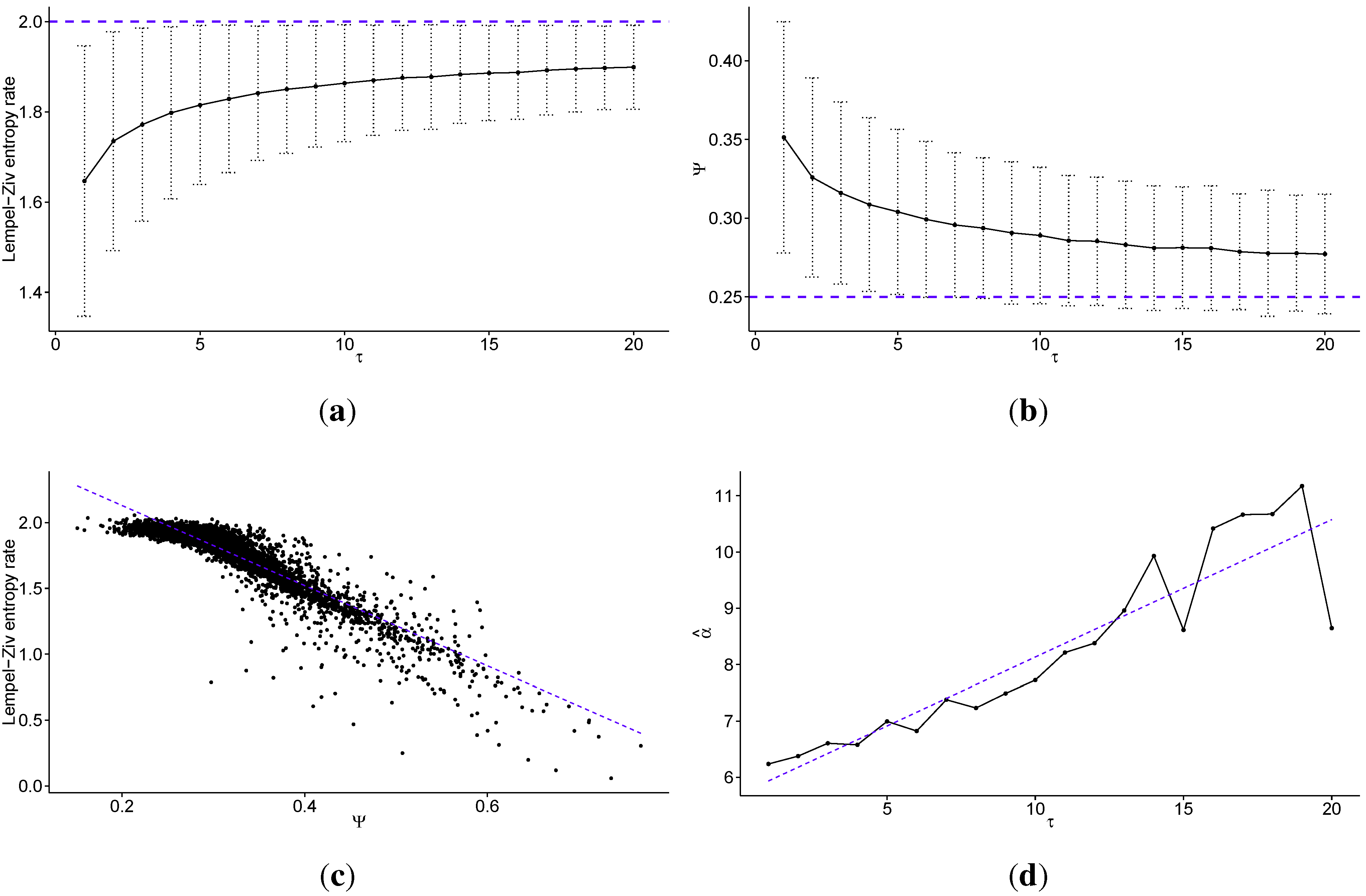
In Figure 1 we present the multiscale entropy analysis results for transaction level logarithmic price change history of 707 stocks from the Warsaw Stock Exchange sampled every τ price changes, discretized into four quantiles ($\Omega =4$). In Figure 1a, we present the Lempel–Ziv entropy rate (average for all studied stocks) as a function of scale τ (the dotted line denotes maximum for fully efficient/unpredictable market; error bars show ± one standard deviation). The Lempel–Ziv entropy, assuming $\Omega =4$, takes values between 0—for fully predictable processes, and 2—for fully random processes (efficient markets). It is important to note that the error bars do not represent estimation errors, but rather the dispersion of the measure on the market (among studied stocks) in terms of standard deviation. Further, the line between the points is strictly to enhance visibility; it is not fitted, but merely connects the points. The values where τ is not an integer are meaningless. Note that the standard errors decrease with increasing τ, and are equal to $0.3$ for $\tau =1$, $0.24$ for $\tau =2$, $0.18$ for $\tau =5$, $0.13$ for $\tau =10$, and $0.09$ for $\tau =20$. In Figure 1b we present the percentage of times the Maximum Entropy Production Principle correctly guesses the quantile of the next price change (Ψ—average for all studied stocks) as a function of scale τ (the dotted line denotes value that would be obtained with random guessing; error bars show ± one standard deviation). Note that the standard errors decrease with increasing τ, and are equal to $0.07$ for $\tau =1$, $0.06$ for $\tau =2$, $0.05$ for $\tau =5$, $0.04$ for $\tau =10$ and $\tau =20$. In Figure 1c we present the correlation between the Lempel–Ziv entropy rate and Ψ for all studied scales (with linear fit visible as the dotted line), to show how these two measures are related.

Regardless of the used scale parameter, analysts may be interested in the stocks for which the predictability (measured by either method) is the highest. In other words, they pay close attention to the tail of the distribution, or where the interesting stocks are situated within this picture. This is why we fit a power law distribution to the empirically obtained values of Ψ for all studied stocks, for each of the scale parameters τ. We obtained a relatively good fit (on the verge of significance at 5% using Kolmogorov-Smirnov test), and thus we can say the distribution of Ω is characterised by fat tails, even if they do not strictly follow a power law. We are not interested in a perfect fit of a particular distribution, but rather in how steep the slope of these fat tails is with respect to the scale τ. In Figure 1d, we present the scaling parameter of the power law fitted for Ψ as a function of scale τ (with linear fit visible as the dotted line). The distributions themselves, for a few values of scale τ, are presented in Figure 2. For the description of the power law distribution ($p\left(x\right)=\frac{\alpha -1}{x_{min}}{\left(\frac{x}{x_{min}}\right)}^{-\alpha }$) and how to estimate its parameters, please see [36,37]. Fitting and associated tests have been performed using poweRlaw package in R.

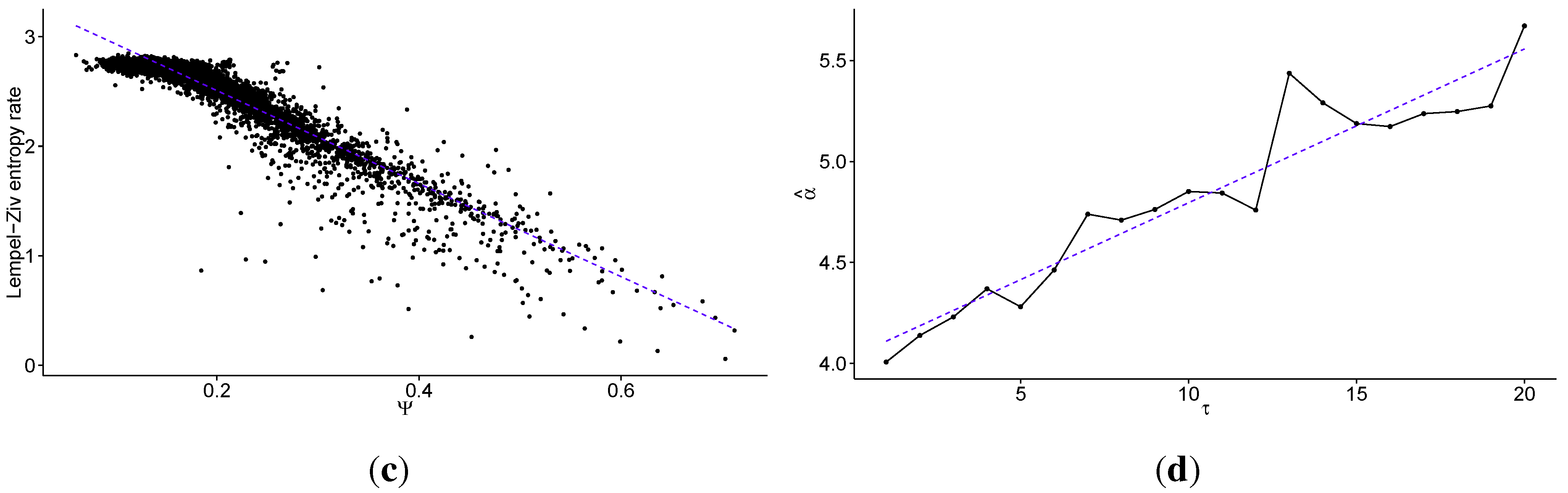
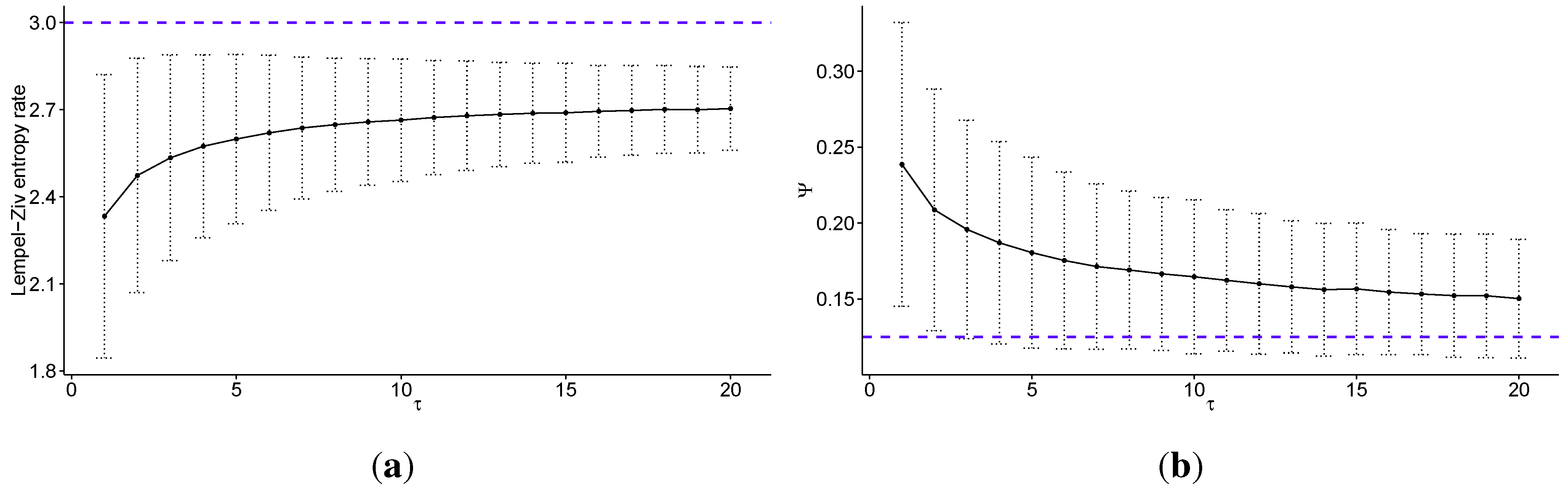
In Figure 3 we present the same results as in Figure 1, but with the data discretized into eight quantiles ($\Omega =8$). Such discretization carries more information about the level of volatility than when using $\Omega =4$, but the distinction between states beecome blurred and are not as clear, especially intuitively. Please note that the Lempel–Ziv entropy rate takes values between 0 and 3 for $\Omega =8$. Note that the standard errors for Lempel-Ziv entropy rates decrease with increasing τ, and are equal to $0.49$ for $\tau =1$, $0.4$ for $\tau =2$, $0.29$ for $\tau =5$, $0.21$ for $\tau =10$, and $0.14$ for $\tau =20$. Standard errors for Ψ also decrease, and are equal to $0.09$ for $\tau =1$, $0.08$ for $\tau =2$, $0.06$ for $\tau =5$, $0.05$ for $\tau =10$, and $0.04$ for $\tau =20$.

Figure 1. Multiscale analysis of transaction level logarithmic price change history for 707 stocks from the Warsaw Stock Exchange sampled every τ price changes, discretized into four quantiles: (a) the average Lempel–Ziv entropy rate among studied stocks as a function of scale τ (the dotted line denotes the maximum for fully efficient/unpredictable market; error bars show ± one standard deviation); (b) the percentage of times the Maximum Entropy Production Principle correctly guesses the quantile of the next price change (Ψ) averaged over all studied stocks as a function of scale τ (the dotted line denotes the value which would be obtained with random guessing; error bars show ± one standard deviation); (c) the correlation between the Lempel–Ziv entropy rate and Ψ for all studied stocks and scales (the dotted line shows a linear fit); (d) the scaling parameter of the power law fitted for Ψ as a function of scale τ (the dotted line shows a linear fit). We observe that the predictability of the stock price changes decreases fast with increasing time scale, both with regard to theoretical measure of Lempel–Ziv entropy and practical test for the Maximum Entropy Production Principle. In fact the Pearson’s correlation coefficient between these two measures is $-0.9256$ for all studied scales. Further, we observe that in general the scaling parameter of the power law fitted to the tails of the distributions of Ψ increases with the time scale τ, that is the predictability decays faster for larger values of τ.

Figure 1. Multiscale analysis of transaction level logarithmic price change history for 707 stocks from the Warsaw Stock Exchange sampled every τ price changes, discretized into four quantiles: (a) the average Lempel–Ziv entropy rate among studied stocks as a function of scale τ (the dotted line denotes the maximum for fully efficient/unpredictable market; error bars show ± one standard deviation); (b) the percentage of times the Maximum Entropy Production Principle correctly guesses the quantile of the next price change (Ψ) averaged over all studied stocks as a function of scale τ (the dotted line denotes the value which would be obtained with random guessing; error bars show ± one standard deviation); (c) the correlation between the Lempel–Ziv entropy rate and Ψ for all studied stocks and scales (the dotted line shows a linear fit); (d) the scaling parameter of the power law fitted for Ψ as a function of scale τ (the dotted line shows a linear fit). We observe that the predictability of the stock price changes decreases fast with increasing time scale, both with regard to theoretical measure of Lempel–Ziv entropy and practical test for the Maximum Entropy Production Principle. In fact the Pearson’s correlation coefficient between these two measures is $-0.9256$ for all studied scales. Further, we observe that in general the scaling parameter of the power law fitted to the tails of the distributions of Ψ increases with the time scale τ, that is the predictability decays faster for larger values of τ.

Figure 2. Power law distributions (on a log-log scale) fitted for the percentage of times the Maximum Entropy Production Principle correctly guesses the quantile of the next price change (Ψ) based on transaction level logarithmic price change history for 707 stocks from Warsaw Stock Exchange sampled every τ price changes, discretized into four quantiles, for different values of τ: (a) $\tau =1$; (b) $\tau =5$; (c) $\tau =10$; (d) $\tau =20$. We observe that in general, the scaling parameter of the power law fitted to the tails of the distributions of Ψ increases with the time scale τ, that is, the predictability decays faster for larger values of τ, which is consistent with our other findings.

Figure 2. Power law distributions (on a log-log scale) fitted for the percentage of times the Maximum Entropy Production Principle correctly guesses the quantile of the next price change (Ψ) based on transaction level logarithmic price change history for 707 stocks from Warsaw Stock Exchange sampled every τ price changes, discretized into four quantiles, for different values of τ: (a) $\tau =1$; (b) $\tau =5$; (c) $\tau =10$; (d) $\tau =20$. We observe that in general, the scaling parameter of the power law fitted to the tails of the distributions of Ψ increases with the time scale τ, that is, the predictability decays faster for larger values of τ, which is consistent with our other findings.

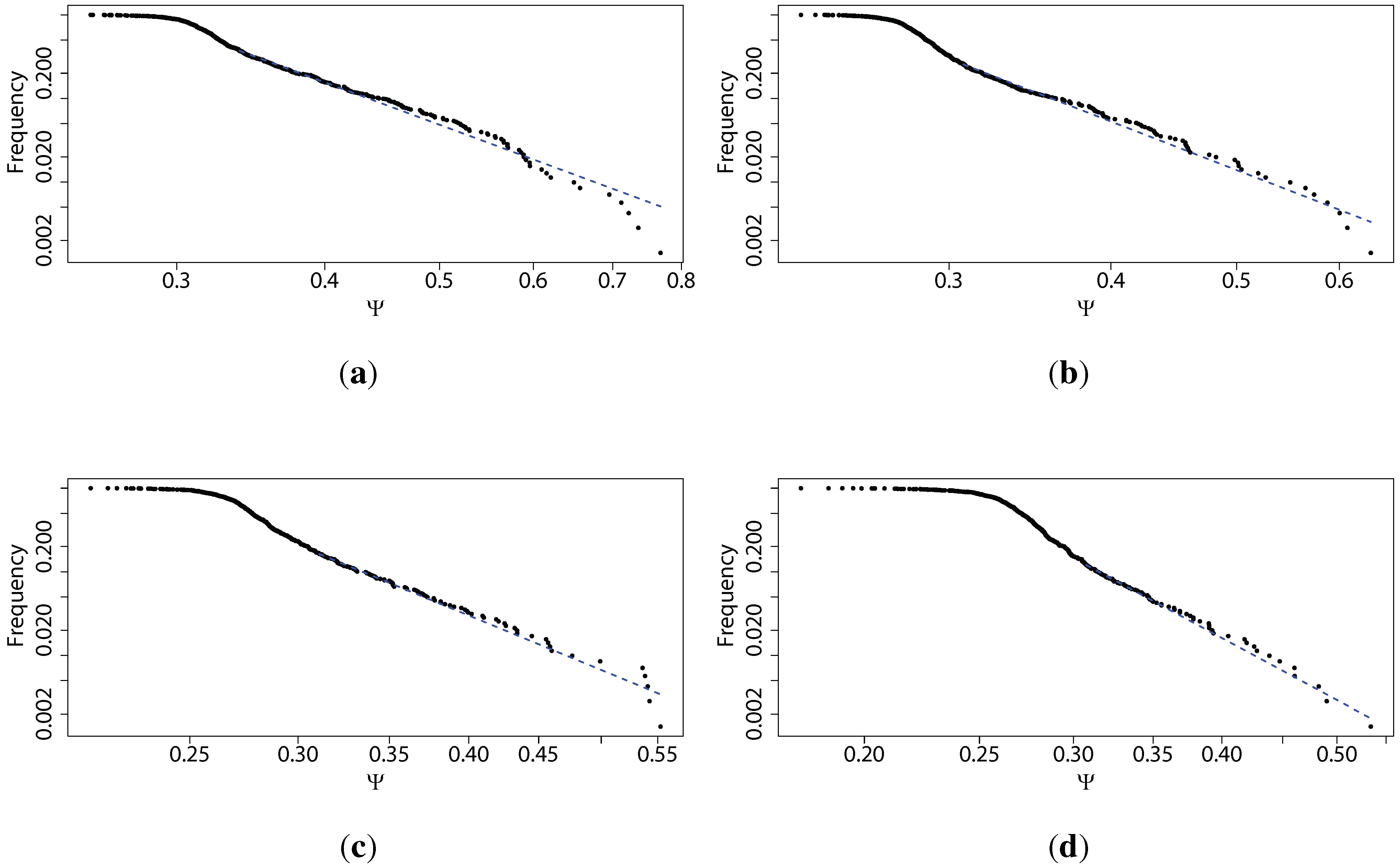
Figure 3. Multiscale analysis of transaction level logarithmic price change history for 707 stocks from Warsaw Stock Exchange sampled every τ price changes, discretized into eight quantiles: (a) the average Lempel–Ziv entropy rate among studied stocks as a function of scale τ (the dotted line denotes maximum for fully efficient/unpredictable market; error bars show ± one standard deviation); (b) the percentage of times the Maximum Entropy Production Principle correctly guesses the quantile of the next price change (Ψ) averaged over all studied stocks as a function of scale τ (the dotted line denotes the value which would be obtained with random guessing; error bars show ± one standard deviation); (c) the correlation between the Lempel–Ziv entropy rate and Ψ for all studied stocks and scales (with linear fit visible as the dotted line); (d) the scaling parameter of the power law fitted for Ψ as a function of scale τ (the dotted line shows a linear fit). We observe that the predictability of the stock price changes decreases fast with increasing time scale, both with regard to theoretical measure of Lempel–Ziv entropy and practical test for the Maximum Entropy Production Principle. In fact the Pearson’s correlation coefficient between these two measures is equal to $-0.9414$ for all studied scales. Further, we observe that in general the scaling parameter of the power law fitted to the tails of the distributions of Ψ increases with the time scale τ, that is the predictability decays faster for larger values of τ.

Figure 3. Multiscale analysis of transaction level logarithmic price change history for 707 stocks from Warsaw Stock Exchange sampled every τ price changes, discretized into eight quantiles: (a) the average Lempel–Ziv entropy rate among studied stocks as a function of scale τ (the dotted line denotes maximum for fully efficient/unpredictable market; error bars show ± one standard deviation); (b) the percentage of times the Maximum Entropy Production Principle correctly guesses the quantile of the next price change (Ψ) averaged over all studied stocks as a function of scale τ (the dotted line denotes the value which would be obtained with random guessing; error bars show ± one standard deviation); (c) the correlation between the Lempel–Ziv entropy rate and Ψ for all studied stocks and scales (with linear fit visible as the dotted line); (d) the scaling parameter of the power law fitted for Ψ as a function of scale τ (the dotted line shows a linear fit). We observe that the predictability of the stock price changes decreases fast with increasing time scale, both with regard to theoretical measure of Lempel–Ziv entropy and practical test for the Maximum Entropy Production Principle. In fact the Pearson’s correlation coefficient between these two measures is equal to $-0.9414$ for all studied scales. Further, we observe that in general the scaling parameter of the power law fitted to the tails of the distributions of Ψ increases with the time scale τ, that is the predictability decays faster for larger values of τ.

4. Discussion

Looking at Figure 1, we observe that the predictability of the stock price changes decreases quickly with increasing time scale, both with regard to theoretical measure of Lempel–Ziv entropy and a practical test for the Maximum Entropy Production Principle. In fact, the Pearson’s correlation coefficient between these two measures is equal to $-0.9256$ for all studied scales. However, we note that it is not a fully linear relationship. For stocks with a high entropy rate, there is little correlation, and this correlation only appears strong for less efficient stocks. This is not a drawback, as we are interested in what happens with these inefficiencies. Further, this correlation is somewhat surprising, given that the Maximum Entropy Production Principle guesses the next price change to be the one that is the closest to efficient market behaviour, and yet it gives the best results for time series characterised by the largest predictability (that is, ones furthest from the market efficiency). Nonetheless, thanks to such a large correlation coefficient, this study adds to the efforts to bridge the gap between profitability and predictability, which have yielded poor results so far (though the principle by no means guarantees profitability, though it constructs a mechanism for market inefficiencies stemming from the market’s stubborn insistence on trying to become efficient at all times). We note that further studies will be required to test whether trading strategies based on this principle can really be profitable, though this study appears to suggest that it may be the case, if only for intraday trading.

For large values of the time scale τ, the predictability of the logarithmic returns on Warsaw’s market is not statistically significantly distinct from the fully efficient case (which would be characterised by an entropy rate of 2, as shown in Figure 1a), and the standard deviation is not reaching 2 mostly due to slight bias. Conversely, the correct guessing rate (Ψ) of Maximum Entropy Production Principle is larger than one obtained by guessing at random, though the difference is not statistically significant for large values of τ, as seen in Figure 1b. Both measures show the same dependence of predictability on the time scale τ, which is that the predictability of log returns decays quickly with increasing time scale. The biggest decay occurs for values of τ smaller than 5, and thus we can say that most of the inefficiencies of the price formation processes on Warsaw’s market occur at time scales below five price changes for a given security. Therefore, one can argue that high-frequency intraday trading should be significantly more profitable than slower trading, assuming the trader can use these inefficiencies of the market to obtain a comparative advantage against his competitors. The fast dissipation of these instantaneous market non-equilibria can be explained quite easily. The longer they persist, the easier it is for market participants to spot them and use them for profit. Thus, there is market pressure for finding them and using them as quickly as possible. Consequently, they are virtually non-existent at large time scales. As we can see in the results, it may take up to a few price changes on a given security before they dissipate, leaving some room for market speculation.

Further, we fit a power law to the tail of the distributions of Ψ, and find a relatively good fit (confirmed by Kolmogorov–Smirnov test results above), thus confirming that these distributions are characterised by fat tails. We note that it is irrelevant whether the distribution is precisely scale free or follows a slightly different distribution (i.e., log-normal). The main point is to show that it is strongly fat tailed. We observe that in general the scaling parameter of the power law fit to the tails of the distributions of Ψ increases with the time scale τ, which is that the predictability decays faster for larger values of τ. Looking at Figure 2, we observe that in general the scaling parameter of the power law fit to the tails of the distributions of Ψ increases with the time scale τ, which is that the predictability decays faster for larger values of τ, consistent with our other findings. These results can be explained by the fact that the whole market cannot be strongly inefficient, as it would be a fragile state. These results also mean that analysts will find fewer predictable securities at large time scales, but the distribution of predictability on all scales is characterised by fat tails, and consequently the analysts can easily spot the most predictable securities and concentrate on them.

Strikingly, the multiscale entropy characteristic of the Warsaw Stock Exchange presented in Figure 1a is a mirror image (opposite) of the multiscale entropy characteristic of white noise (as portrayed in [20]). Thus, we see that the financial time series describing logarithmic stock price changes behave in quite a different manner from white noise, at least in its information-theoretic characteristics. Returning to the Efficient-Market Hypothesis, if we assume that a market is indeed efficient (the weak form of the hypothesis), then the stock price follows a random walk, which is that the time series of log returns a white noise process. Even if this is not a completely precise depiction of the hypothesis, since the complete opposite appears to be the case, it is clear that the market in Warsaw is not efficient in this way. Such striking opposition to the characteristics of white noise also calls into question financial models using Brownian motion, as they are closely related to white noise (white noise is the generalised mean-square derivative of the Brownian motion). In fact, in our earlier studies we have obtained results hinting that agent-based models approximate the information-theoretic characteristics of logarithmic returns on financial markets better than approaches based on Brownian motion or Lévy processes.

Finally, looking at results obtained for data discretized into a different number of quantiles, we can see that the results are generally robust with respect to the choice of the number of quantiles used in the discretization step. There are a few notes to make regarding this observation, however. In the analysis performed for data discretized into two quantiles, we observed more erratic behaviour than expected, since such a procedure loses all information about the volatility of the price changes. Thus, we have not presented these results. In addition to the above, the usage of quartiles hints at another feature of this study. When discretizing returns, we ignored outliers in the analysis. As such, this setup investigates the normal operations of financial markets and ignores Dragon King or Black Swan effects, and is not designed to predict extreme behaviour of the market. Consequently, fat tails of financial returns do not influence the analysis very strongly. However, we find the volatility clustering to strongly influence the above results [38].

5. Conclusions

We have presented a multiscale entropy analysis of predictability measures applied to a database of transaction-level logarithmic stock returns from the Warsaw Stock Exchange. We have estimated Shannon’s entropy rate using the Lempel–Ziv algorithm, and have also used the Maximum Entropy Production Principle as a more constructive framework. Both of those measures are highly correlated, but while the former only refutes the Efficient-Market Hypothesis at very short time scales, the latter also constructs a principle underlying the price formation processes to take its place. This principle at least attempts to move the analysis of predictability in the direction of its relationship with profitability. While further research is needed to answer the question of the profitability of a strategy based on the principle of maximal entropy production, the results presented in this paper suggest that such strategies may be effective for trading with very short time horizons. Our results indicate that price formation processes for stocks on Warsaw’s market are significantly inefficient at very small scales, but these inefficiencies dissipate quickly and are relatively small at time scales over 5 price changes. Further, we have shown that the predictability of stock price changes follows a fat tailed distribution, and thus there exist some predictable price formation processes for some stocks. Strikingly, the multiscale entropy analysis presented in this study shows that price formation processes exhibit a completely opposite information-theoretic characteristic to white noise, calling into question methods in finance based on Brownian motion or Lévy processes. Further studies should confirm these findings on other markets, both in terms of different securities and different stock exchanges, and expand the robustness of the analysis presented in this study.

References

- P.A. Samuelson. “Proof That Properly Anticipated Prices Fluctuate Randomly.” Ind. Manag. Rev. 6 (1965): 41–49. [Google Scholar]
- B. Rosser. “Econophysics and Economic Complexity.” Adv. Complex Syst. 11 (2008): 745–760. [Google Scholar] [CrossRef]
- C.C. Lee, and J. Lee. “Energy prices, multiple structural breaks, and efficient market hypothesis.” Appl. Energy 86 (2009): 466–479. [Google Scholar] [CrossRef]
- G. Yen, and C.F. Lee. “Efficient Market Hypothesis (EMH): Past, Present and Future.” Rev. Pac. Basin Financ. Mark. Policies 11 (2008): 305–329. [Google Scholar] [CrossRef]
- E. Peters. Chaos and Order in the Capital Markets. New York, NY, USA: Wiley, 1991. [Google Scholar]
- U. Muller, M. Dacorogna, R. Dave, O. Pictet, R. Olsen, and J. Ward. Fractals and intrinsic time—A challenge to econometricians, Olsen and Associates, Jacksonville, FL, USA, 1993.
- A. Lo. “The Adaptive Markets Hypothesis: Market Efficiency from an Evolutionary Perspective.” J. Portf. Manag. 30 (2004): 15–29. [Google Scholar] [CrossRef]
- B.B. Mandelbrot. “The Variation of Certain Speculative Prices.” J. Bus. 36 (1963): 394–419. [Google Scholar] [CrossRef]
- L.P. Kadanoff. “From Simulation Model to Public Policy: An Examination of Forrester’s Urban Dynamics.” Simulation 16 (1971): 261–268. [Google Scholar] [CrossRef]
- R.N. Mantegna. “Levy Walks and Enhanced Diffusion in Milan Stock Exchange.” Physica A 179 (1991): 232–242. [Google Scholar] [CrossRef]
- P. Fiedor. “Frequency Effects on Predictability of Stock Returns.” In Proceedings of the IEEE Computational Intelligence for Financial Engineering & Economics 2014; Edited by A. Serguieva, D. Maringer, V. Palade and R.J. Almeida. London, UK: IEEE, 2014, pp. 247–254. [Google Scholar]
- C.E. Shannon. “A Mathematical Theory of Communication.” Bell Syst. Tech. J. 27 (1948): 379–423, 623–656. [Google Scholar] [CrossRef]
- P. Fiedor. “Maximum Entropy Production Principle for Stock Returns.” ArXiV 1408.3728, 2014. [Google Scholar]
- Y. Wu, S.H.K. Tang, X.M. Fan, and N. Groenewold. The Chinese Stock Market: Efficiency, Predictability And Profitability. Cheltenham, UK: Edward Elgar Publishing, 2004. [Google Scholar]
- R. Rothenstein, and K. Pawelzik. “Limited profit in predictable stock markets.” Physica A 348 (2005): 419–427. [Google Scholar] [CrossRef]
- N. Navet, and S.H. Chen. “On Predictability and Profitability: Would GP Induced Trading Rules be Sensitive to the Observed Entropy of Time Series? ” In Natural Computing in Computational Finance. Edited by T. Brabazon and M. O’Neill. Berlin/Heidelberg, Germany: Springer, 2008, Volume 100, Studies in Computational Intelligence. [Google Scholar]
- C. Aghamohammadi, M. Ebrahimian, and H. Tahmooresi. “Permutation approach, high frequency trading and variety of micro patterns in financial time series.” Physica A 413 (2014): 25–30. [Google Scholar] [CrossRef]
- E. Rodriguez, M. Aguilar-Cornejo, R. Femat, and J. Alvarez-Ramirez. “US stock market efficiency over weekly, monthly, quarterly and yearly time scales.” Physica A 413 (2014): 554–564. [Google Scholar] [CrossRef]
- C.A. Zapart. “Econophysics: A challenge to econometricians.” Physica A 419 (2015): 318–327. [Google Scholar] [CrossRef]
- M. Costa, A. Goldberger, and C.K. Peng. “Multiscale entropy analysis of physiologic time series.” Phys. Rev. Lett. 89 (2002): 062102. [Google Scholar] [CrossRef]
- M. Costa, A. Goldberger, and C.K. Peng. “Multiscale entropy analysis of biological signals.” Phys. Rev. E 71 (2005): 021906. [Google Scholar] [CrossRef]
- T. Cover, and J. Thomas. Elements of Information Theory. New York, NY, USA: John Wiley & Sons, 1991. [Google Scholar]
- Y. Sinai. “On the Notion of Entropy of a Dynamical System.” Dokl. Akad. Nauk SSSR 124 (1959): 768–771. [Google Scholar]
- A.N. Kolmogorov. “Entropy per unit time as a metric invariant of automorphism.” Dokl. Akad. Nauk SSSR 124 (1959): 754–755. [Google Scholar]
- Y. Gao, I. Kontoyiannis, and E. Bienenstock. “From the entropy to the statistical structure of spike trains.” In Proceedings of the IEEE International Symposium on Information Theory, Seattle, United States, 6–12 July 2006; pp. 645–649.
- M. Farah, M. Noordewier, S. Savari, L. Shepp, A. Wyner, and J. Ziv. “On the entropy of DNA: Algorithms and measurements based on memory and rapid convergence.” In SODA’95: Proceedings of the Sixth Annual ACM-SIAM Symposium on Discrete Algorithms; Society of Industrial and Applied Mathematics, San Francisco, United States, 22-24 January 1995; pp. 48–57.
- I. Kontoyiannis, P. Algoet, Y. Suhov, and A. Wyner. “Nonparametric entropy estimation for stationary processes and random fields, with applications to English text.” IEEE Trans. Inf. Theory 44 (1998): 1319–1327. [Google Scholar] [CrossRef]
- A. Lempel, and J. Ziv. “A Universal Algorithm for Sequential Data Compression.” IEEE Trans. Inf. Theory 23 (1977): 337–343. [Google Scholar]
- F. Willems, Y. Shtarkov, and T. Tjalkens. “The Context-Tree Weighting Method: Basic Properties.” IEEE Trans. Inf. Theory 41 (1995): 653–664. [Google Scholar] [CrossRef]
- M. Kennel, J. Shlens, H. Abarbanel, and E. Chichilnisky. “Estimating entropy rates with Bayesian confidence intervals.” Neural Comput. 17 (2005): 1531–1576. [Google Scholar] [CrossRef] [PubMed]
- G. Louchard, and W. Szpankowski. “On the average redundancy rate of the Lempel–Ziv code.” IEEE Trans. Inf. Theory 43 (1997): 2–8. [Google Scholar] [CrossRef]
- F. Leonardi. “Some upper bounds for the rate of convergence of penalized likelihood context tree estimators.” Braz. J. Probab. Stat. 24 (2010): 321–336. [Google Scholar] [CrossRef]
- I. Kontoyiannis. “Asymptotically Optimal Lossy Lempel–Ziv Coding.” In IEEE International Symposium on Information Theory. Cambridge, MA, USA: MIT, 1998. [Google Scholar]
- Y. Gao, I. Kontoyiannis, and E. Bienenstock. “Estimating the Entropy of Binary Time Series: Methodology, Some Theory and a Simulation Study.” Entropy 10 (2008): 71–99. [Google Scholar] [CrossRef]
- R. Steuer, L. Molgedey, W. Ebeling, and M. Jimenez-Montaño. “Entropy and Optimal Partition for Data Analysis.” Eur. Phys. J. B 19 (2001): 265–269. [Google Scholar] [CrossRef]
- A. Muniruzzaman. “On measures of location and dispersion and test of hypothesis on a Pareto distribution.” Calc. Stat. Assoc. Bull. 7 (1957): 115–123. [Google Scholar]
- A. Clauset, C. Shalizi, and M. Newman. “Power-law distributions in empirical data.” SIAM Rev. 51 (2009): 661–703. [Google Scholar] [CrossRef]
- P. Fiedor. “Information-theoretic approach to lead-lag effect on financial markets.” Eur. Phys. J. B 87 (2014): 1–9. [Google Scholar] [CrossRef]
© 2015 by the author; licensee MDPI, Basel, Switzerland. This article is an open access article distributed under the terms and conditions of the Creative Commons Attribution license (http://creativecommons.org/licenses/by/4.0/).
Share and Cite
MDPI and ACS Style
Fiedor, P. Multiscale Analysis of the Predictability of Stock Returns. Risks 2015, 3, 219-233. https://doi.org/10.3390/risks3020219
AMA Style
Fiedor P. Multiscale Analysis of the Predictability of Stock Returns. Risks. 2015; 3(2):219-233. https://doi.org/10.3390/risks3020219
Chicago/Turabian StyleFiedor, Paweł. 2015. "Multiscale Analysis of the Predictability of Stock Returns" Risks 3, no. 2: 219-233. https://doi.org/10.3390/risks3020219