When the U.S. Stock Market Becomes Extreme?

Abstract
:1. Introduction
2. Methodology
2.1. Tail Distribution
2.2. Threshold Selection
2.3. Three Extreme Risk Management Measures
3. Data Analysis
3.1. Data Description
3.2. Data Filtering Process

| Z | Z | ||
|---|---|---|---|
| Mean | −0.0032 | Q5 (residual) | 2.9403 |
| (p-value) | (0.401) | ||
| Median | 0.0202 | Q5 (squared residual) | 7.2983 * |
| (p-value) | (0.063) | ||
| Maximum | 7.0191 | Q10 (residual) | 11.504 |
| (p-value) | (0.175) | ||
| Minimum | −13.1417 | Q10 (squared residual) | 11.546 |
| (p-value) | (0.173) | ||
| Std. Dev. | 1.0001 | Q20 (residual) | 20.090 |
| (p-value) | (0.328) | ||
| Skewness | −0.5062 | Q20 (squared residual) | 16.385 |
| (Z-statistic, p-value) | (−16.2613, 2.2×10⁻¹⁶) | (p-value) | (0.566) |
| Kurtosis | 7.8954 | μ | 0.0002 *** |
| (Z-statistic, p-value) | (36.6956, 2.2×10⁻¹⁶) | (Z-statistic) | (4.7722) |
| Jarque–Bera | 16607.86 *** | −0.0812 | |
| (p-value) | (0.0000) | (Z-statistic) | (−1.0679) |
| Engle LM (1) | 6.0183 ** | 0.1853 ** | |
| (p-value) | (0.0142) | (Z-statistic) | (2.4722) |
| Engle LM (2) | 6.3745 ** | ω | 9.37e-07 *** |
| (p-value) | (0.0413) | (Z-statistic) | (15.5038) |
| Engle LM (5) | 7.2949 * | α | 0.0306 *** |
| (p-value) | (0.1996) | (Z-statistic) | (13.0564) |
| Engle LM (10) | 11.4924 | γ | 0.0884 *** |
| (p-value) | (0.3205) | (Z-statistic) | (28.0765) |
| q1% | −2.5373 | β | 0.9154 *** |
| (Z-statistic) | (415.2990) | ||
| q5% | −1.6240 | Log-likelihood | 54439.85 |
| q95% | 1.5658 | Akaike criterion | −6.8220 |
| q99% | 2.3426 | Number | 15950 |

3.3. Descriptive Statistics
3.4. Quantile Regression
4. Empirical Findings
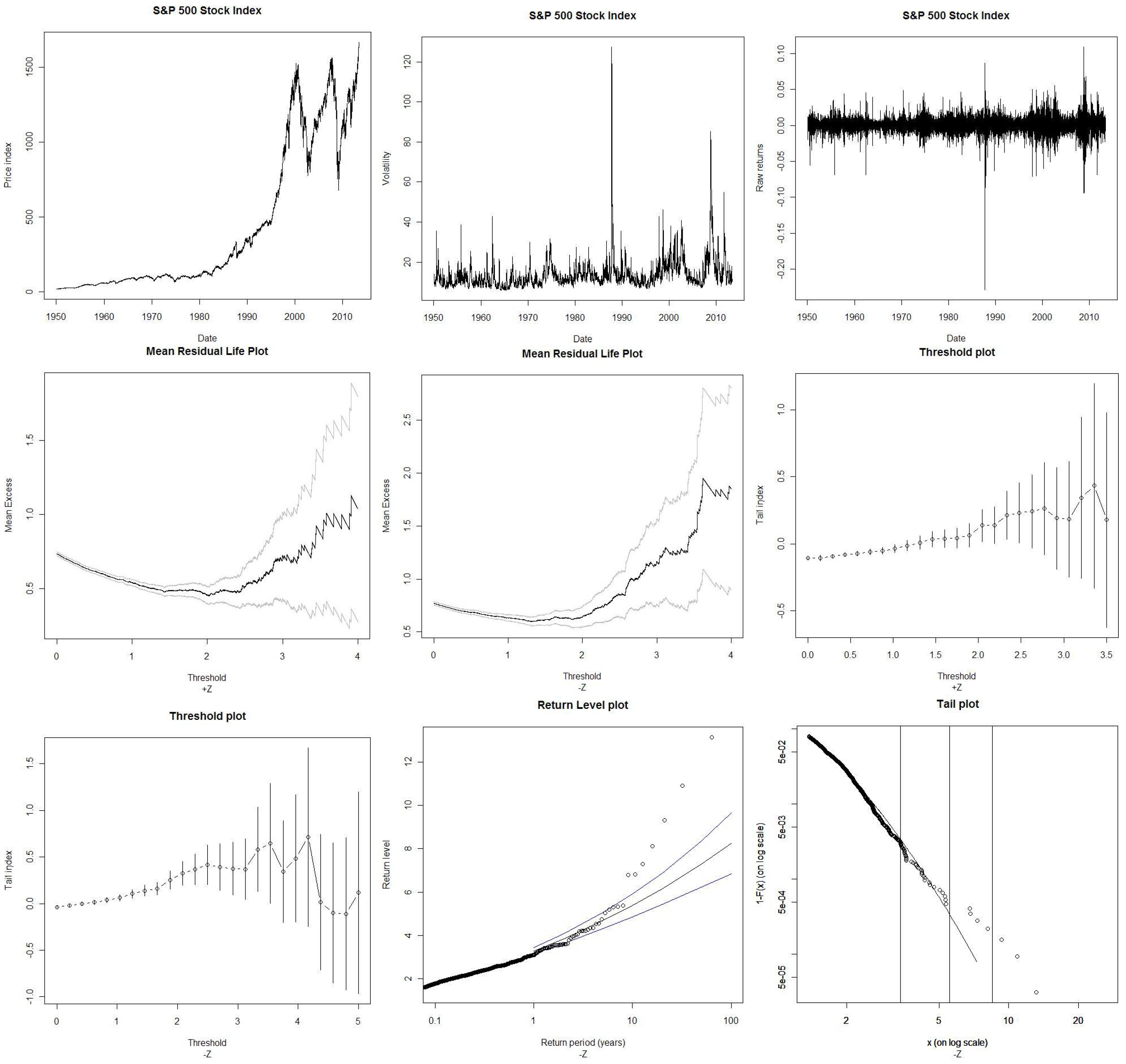
4.1. Threshold Selection Results
| Mean residual life plot | +1.20 | −1.40 |
| Threshold plot | [+0.09; +1.50] | [−0.80; −1.80] |
| Optimal selection | +0.9388 | −1.3735 |
4.2. Tail Characteristics
| ξ | −0.0411 *** | 0.1359 *** |
| (s.e) | (0.0143) | (0.0274) |
| β | 0.5671 *** | 0.5168 *** |
| (s.e) | (0.0140) | (0.0201) |
| Threshold | +0.9388 | −1.3735 |
| Nb. Exceedances | 2443 | 1278 |
| Percentile | 0.8468 | 0.9198 |
| Neg. Lik. | 957.047 | 608.1859 |
4.3. The Extreme Downside Risk
| Probability | VaR-GPD | ES-GPD | VaR-normal | ES-normal |
|---|---|---|---|---|
| 0.9900 | −2.6166 | −3.4104 | −2.3263 | −2.6652 |
| 0.9950 | −3.1151 | −3.9873 | −2.5758 | −2.8919 |
| 0.9990 | −4.4709 | −5.5564 | −3.0902 | −3.3670 |
| 0.9995 | −5.1526 | −6.3454 | −3.2905 | −3.5543 |
| 0.9999 | −7.0068 | −8.4912 | −3.7190 | −3.9584 |
| Period | Lower bound | Upper bound | Lower bound | Upper bound | ||
|---|---|---|---|---|---|---|
| 1 | 2.8586 | 2.7746 | 2.9425 | −3.2857 | −3.1384 | −3.4330 |
| 2 | 3.1921 | 3.0833 | 3.3008 | −3.8502 | −3.6283 | −4.0720 |
| 5 | 3.6186 | 3.4683 | 3.7689 | −4.6829 | −4.3138 | −5.0519 |
| 10 | 3.9307 | 3.7426 | 4.1188 | −5.3854 | −4.8609 | −5.9098 |
| 20 | 4.2340 | 4.0031 | 4.4649 | −6.1572 | −5.4325 | −6.8819 |
| 50 | 4.6219 | 4.3271 | 4.9166 | −7.2958 | −6.2255 | −8.3661 |
| 100 | 4.9057 | 4.5577 | 5.2537 | −8.2564 | −6.8526 | −9.6601 |
4.4. EVT with Raw Returns
4.5. Robustness Check
5. Conclusions
Conflicts of Interest
References
- J. Danielsson, and C.G. de Vries. “Tail index quantile estimation with very high frequency data.” J. Empir. Financ. 4 (1997): 241–257. [Google Scholar] [CrossRef]
- J. Danielsson, L. de Haan, L. Peng, and C.G. de Vries. “Using a bootstrap method to choose the sample fraction in tail index estimation.” J. Multivar. Anal. 76 (2001): 226–248. [Google Scholar] [CrossRef]
- J. Danielsson, and Y. Morimoto. “Forecasting extreme financial risk: A critical analysis of practical methods for the Japanese market.” Monet. Econ. Stud. 12 (2000): 25–48. [Google Scholar]
- R. Gencay, F. Selcuk, and A. Ulugulyagci. “High volatility, thick tails and extreme value theory in value-at-risk estimation.” Math. Econ. 33 (2003): 337–356. [Google Scholar] [CrossRef]
- G. Gettinby, C.D. Sinclair, D.M. Power, and R.A. Brown. “An analysis of the distribution of extremes in indices of share returns in the US, UK and Japan from 1963 to 2000.” Int. J. Financ. Econ. 11 (2006): 97–113. [Google Scholar] [CrossRef]
- M. Gilli, and E. Kellezi. Extreme Value Theory for Tail-Related Risk Measure. Working Paper; Geneva, Switzerland: University of Geneva, 2000. [Google Scholar]
- E. Jondeau, and M. Rockinger. “Testing for differences in the tails of stock market returns.” J. Empir. Financ. 10 (2003): 559–581. [Google Scholar] [CrossRef]
- B. LeBaron, and R. Samanta. Extreme Value Theory and Fat Tails in Equity Markets. Working Paper; Waltham, MA, USA: Brandeis University, 2004. [Google Scholar]
- F. Longin. “The asymptotic distribution of extreme stock market returns.” J. Bus. 69 (1996): 383–408. [Google Scholar] [CrossRef]
- F. Longin. “Stock market crashes: Some quantitative results based on extreme value theory.” Deriv. Use Trading Regul. 7 (2001): 197–205. [Google Scholar]
- A.J. McNeil, and T. Saladin. “Developing scenarios for future extreme losses using the POT model.” In Extremes and Integrated Risk Management. London, UK: RISK Books, 1998. [Google Scholar]
- A.J. McNeil. Extreme Value Theory for Risk Managers. Working Paper; Zürich, Switzerland: University of Zurich, 1999. [Google Scholar]
- A.J. McNeil, and R. Frey. “Estimation of tail-related risk measures for heteroskedastic financial time series: An extreme value approach.” J. Empir. Financ. 7 (2000): 271–300. [Google Scholar] [CrossRef]
- K. Tolikas, and R.A. Brown. The Distribution of the Extreme Daily Returns in the Athens Stock Exchange. Working Paper; Dundee, UK: University of Dundee, 2005. [Google Scholar]
- J. Beirlant, Y. Goegebeur, J. Segers, and J. Teugels. Statistics of Extremes: Theory and Applications. Chichester, UK: Wiley, 2004. [Google Scholar]
- P. Embrechts, C. Klüppelberg, and T. Mikosch. Modelling Extremal Events for Insurance and Finance. New York, NY, USA: Springer, 1997. [Google Scholar]
- R. Koenker, and G. Bassett. “Regression quantiles.” Econometrica 46 (1978): 33–50. [Google Scholar] [CrossRef]
- R. Koenker, and K. Hallock. “Quantile Regression.” J. Econ. Perspect. 15 (2001): 143–156. [Google Scholar] [CrossRef]
- A. Balkema, and L. de Haan. “Residual life time at great age.” Ann. Probab. 2 (1974): 792–804. [Google Scholar] [CrossRef]
- J.I. Pickands. “Statistical inference using extreme value order statistics.” Ann. Stat. 3 (1975): 119–131. [Google Scholar]
- S.G. Coles. An Introduction to Statistical Modelling of Extreme Values. London, UK: Springer-Verlag, 2001. [Google Scholar]
- E.J. Gumbel. Statistics of Extremes. New-York, NY, USA: Columbia University Press, 1958. [Google Scholar]
- R. Baillie. “The Asymptotic Mean Square Error of multistep prediction from the regression model with autoregressive errors.” J. Am. Stat. Assoc. 74 (1979): 175–184. [Google Scholar] [CrossRef]
- B.M. Hill. “A simple general approach to inference about the tail of a distribution.” Ann. Stat. 3 (1975): 1163–1174. [Google Scholar] [CrossRef]
- C. Acerbi. “Spectral measures of risk: A coherent representation of subjective risk aversion.” J. Bank. Financ. 26 (2002): 1505–1518. [Google Scholar] [CrossRef]
- K. Inui, and M. Kijima. “On the significance of expected shortfall as a coherent risk measure.” J. Bank. Financ. 29 (2005): 853–864. [Google Scholar] [CrossRef]
- K. Kuester, S. Mittik, and M.S. Paolella. “Value-at-risk prediction: A comparison of alternative strategies.” J. Financ. Econ. 4 (2005): 53–89. [Google Scholar] [CrossRef]
- F.C. Martins, and F. Yao. “Estimation of value-at-risk and expected shortfall based on nonlinear models of return dynamics and extreme value theory.” Stud. Nonlinear Dyn. Econ. 10 (2006): 107–149. [Google Scholar] [CrossRef]
- A. Ozun, A. Cifter, and S. Yilmazer. Filtered Extreme Value Theory for Value-at-Risk Estimation. Working Paper; Kadikoy/Istanbul, Turkey: Marmara University, 2007. [Google Scholar]
- Y. Bao, T.-H. Lee, and B. Saltoglu. “Evaluating predictive performance of value-at-risk models in emerging markets: A reality check.” J. Forecast. 25 (2006): 101–128. [Google Scholar] [CrossRef]
- Y. Yamai, and T. Yoshiba. “Value-at-risk versus expected shortfall: A practical perspective.” J. Bank. Financ. 29 (2005): 997–1015. [Google Scholar] [CrossRef]
- P. Artzner, F. Delbaen, J. Eber, and D. Heath. “Coherent measure of risk.” Math. Financ. 9 (1999): 203–228. [Google Scholar] [CrossRef]
- E.J. Gumbel. “The return period of flood flows.” Ann. Math. Stat. 12 (1941): 163–190. [Google Scholar] [CrossRef]
- X. D’Haultfœuille, and P. Givord. La Regression de Quantile en Pratique. Working Paper; Paris, France: Insee, 2010. [Google Scholar]
- G. Bekaert, and G. Wu. “Asymmetric volatility and risk in equity markets.” Rev. Financ. Stud. 13 (2000): 1–42. [Google Scholar] [CrossRef]
- F. Black. “Studies in stock price volatility changes, American Statistical Association.” In Proceedings of the Business and Economic Statistics Section, Boston, MA, USA, 23–26 August, 1976; pp. 177–181.
- J.Y. Campbell, and L. Hentchel. “No news is good news: An asymmetric model of changing volatility in stock returns.” J. Financ. Econ. 31 (1992): 281–318. [Google Scholar] [CrossRef]
- A. Christie. “The stochastic behavior of common stock variances—Value, leverage, and interest rate effects.” J. Financ. Econ. Theory 10 (1982): 407–432. [Google Scholar] [CrossRef]
- 3Note that for the sake of prudence, the return periods of 84 and 27 years correspond to their respective return level absolute upper bound
© 2014 by the author; licensee MDPI, Basel, Switzerland. This article is an open access article distributed under the terms and conditions of the Creative Commons Attribution license (http://creativecommons.org/licenses/by/3.0/).
Share and Cite
Aboura, S. When the U.S. Stock Market Becomes Extreme? Risks 2014, 2, 211-225. https://doi.org/10.3390/risks2020211
Aboura S. When the U.S. Stock Market Becomes Extreme? Risks. 2014; 2(2):211-225. https://doi.org/10.3390/risks2020211
Chicago/Turabian StyleAboura, Sofiane. 2014. "When the U.S. Stock Market Becomes Extreme?" Risks 2, no. 2: 211-225. https://doi.org/10.3390/risks2020211