A Risk Model with an Observer in a Markov Environment

Abstract

We consider a spectrally-negative Markov additive process as a model of a risk process in a random environment. Following recent interest in alternative ruin concepts, we assume that ruin occurs when an independent Poissonian observer sees the process as negative, where the observation rate may depend on the state of the environment. Using an approximation argument and spectral theory, we establish an explicit formula for the resulting survival probabilities in this general setting. We also discuss an efficient evaluation of the involved quantities and provide a numerical illustration.

1. Introduction

In classical risk theory, the ruin of an insurance portfolio is defined as the event that the surplus process becomes negative. In practice, it may be more reasonable to assume that the surplus value is not checked continuously, but at certain times only. If these times are not fixed deterministically, but are assumed to be epochs of a certain independent renewal process, then one often still has sufficient analytical structure to obtain explicit expressions for ruin probabilities and related quantities; see [1,2] for corresponding studies in the framework of the Cramér–Lundberg risk model and Erlang inter-observation times. An alternative ruin concept is studied in [3], where negative surplus does not necessarily lead to bankruptcy, but bankruptcy is declared at the first instance of an inhomogeneous Poisson process with a rate depending on the surplus value, whenever it is negative. When this rate is constant, this bankruptcy concept corresponds to the one in [1,2] for exponential inter-observation times. Yet another related concept is the one of Parisian ruin, where ruin is only reported if the surplus process stays negative for a certain amount of time (see, e.g., [4,5]). If this time is assumed to be an independent exponential random variable instead of a deterministic value, one recovers the former models with exponential inter-observation times and a constant bankruptcy rate function, respectively. Recently, simple expressions for the corresponding ruin probability have been derived when the surplus process follows a spectrally-negative Lévy process, see [6].

In this paper, we extend the above model and allow the surplus process to be a spectrally-negative Markov additive process. The dynamics of such a process change according to an external environment process, modeled by a Markov chain, and changes of the latter may also cause a jump in the surplus process. We assume that the value of the surplus process is only observed at epochs of a Poisson process, and ruin occurs when at any such observation time, the surplus process is negative. We also allow the rate of observations to depend on the current state of the environment (one possible interpretation being that if the environment states refer to different economic conditions, a regulator may increase the observation rates in states of distress). Using an approximation argument and the spectral theory for Markov additive processes, we explicitly calculate for any initial capital the survival probability and the probability to reach a given level before ruin in this model. The resulting formulas turn out to be quite simple. At the same time, these formulas provide information on certain occupation times of the process, which may be of independent theoretical interest.

In Section 2, we introduce the model and the considered quantities in more detail. Section 3 gives a brief summary of general fluctuation results for Markov additive processes that are needed later on. In Section 4, we state our main results and discuss their relation with previous results, and the proofs are given in Section 5. In Section 6, we reconsider the classical ruin concept and show how the present results implicitly extend the classical simple formula for the ruin probability with zero initial capital to the case of a Markov additive surplus process. Finally, in Section 7, we give a numerical illustration of the results for our relaxed ruin concept in a Markov-modulated Cramér–Lundberg model.

2. The Model

Let $\left(X\right(t),J(t\left)\right),t\ge 0$ be a Markov additive process (MAP), where $X\left(t\right)$ is a surplus process and $J\left(t\right)$ is an irreducible Markov chain on n states representing the environment; see, e.g., [7]. While $J\left(t\right)=i$, $X\left(t\right)$ evolves as some Lévy process $X_i\left(t\right)$, and $X\left(t\right)$ has a jump distributed as $U_{ij}$ when $J\left(t\right)$ switches from i to j. Consequently, $X\left(t\right)$ has stationary and independent increments given the corresponding states of the environment. We assume that $X\left(t\right)$ has no positive jumps and that none of the processes, $X_i\left(t\right)$, is a non-increasing Lévy process. The latter assumption is not a real restriction, because one can always remove the corresponding states of $J\left(t\right)$ and replace non-increasing processes by the appropriate negative jumps. Note that the Markov-modulated Cramér–Lundberg risk model with

$$\begin{array}{cc}& X\left(t\right)=u+{\int }_0^t{c}_{J\left(v\right)}dv-\sum _{j=1}^{N\left(t\right)}{Y}_j\hfill \end{array}$$

(1)

is a particular case of the present framework, where u is the initial capital of an insurance portfolio, $c_i>0$ is the premium density in state i, $N\left(t\right)$ is an inhomogeneous Poisson process with claim arrival intensity ${\beta }_i$ in state i and $Y_j$ are independent claim sizes with distribution function $F_i$, if, at the time of occurrence, the environment is in state i (in this case, $U_{ij}\equiv 0$ for all $i,j$); see [7].

Write ${\mathbb{E}}_u[Y;J\left(t\right)]$ for a matrix with $ij$th element $\mathbb{E}\left(Y{1}_{\left\{J\right(t)=j\}}\right|J\left(0\right)=i,X\left(0\right)=u)$, where Y is an arbitrary random variable, and ${\mathbb{P}}_u[A,J\left(t\right)]={\mathbb{E}}_u[1_A;J\left(t\right)]$ for the probability matrix corresponding to an event A. If $u=0$, then we simply drop the subscript. We write $\mathbb{I},\mathbb{O},1,0$ for an identity matrix, a zero matrix, a column vector of ones and a column vector of zeros of dimension n, respectively. For $x\ge 0$, define the first passage time above x (below $-x$) by:

$${\tau }_x^{\pm }=inf\{t\ge 0:\pm X\left(t\right)>x\}$$

As in [2], we assume that ruin occurs when an independent Poissonian observer sees negative $X\left(t\right)$, where, in our setup, the rate of observations depends on the state of $J\left(t\right)$, i.e., the rate is ${\omega }_{J\left(t\right)}\ge 0$ for given ${\omega }_1,\dots ,{\omega }_n$. Recall that a Poisson process of rate ω has no jumps (observations) in some Borel set $B\subset [0,\infty )$ with probability $exp(-\omega {\int }_{B}t̥)$. Hence, the probability of survival (non-ruin) in our model with initial capital u is given by the column vector:

$$\begin{array}{cc}& \varphi \left(u\right)={\mathbb{E}}_u{e}^{-{\sum }_j{\omega }_j{A}_j},\text{where}{A}_j:={\int }_0^{\infty }{1}_{\left\{X\right(t)<0,J(t)=j\}}t̥\hfill \end{array}$$

(2)

which follows by conditioning on the $A_j$s. The ith component of this vector refers to the probability of survival with initial state $J\left(0\right)=i$. Define for any $u\le x$ the $n\times n$ matrix:

$$\begin{array}{cc}& R(u,x):={\mathbb{E}}_u[e^{-{\sum }_j{\omega }_j{A}_j\left(x\right)};J\left({\tau }_x^{+}\right)],\text{with}{A}_j\left(x\right):={\int }_0^{{\tau }_x^{+}}{1}_{\left\{X\right(s)<0,J(s)=j\}}s̥\hfill \end{array}$$

(3)

so $R(u,x)$ is the matrix of probabilities of reaching level x without ruin, when starting at level u.

It is known that $X\left(t\right)/t$ converges to a deterministic constant, μ (the asymptotic drift of $X\left(t\right)$) a.s. as $t\to \infty$, independently of the initial state, $J\left(0\right)$. If $\mu <0$, then $X\left(t\right)\to -\infty$ a.s.; so $A_j\to \infty$ a.s. for all j, and consequently, ruin is certain (unless all ${\omega }_j=0$). If $\mu \ge 0$, then ${\tau }_x^{+}<\infty$ a.s. for all x, and so:

$$\varphi \left(u\right)=\underset{x\to \infty }{lim}R(u,x)1$$

Finally, note that $R(u,x)$ can be interpreted as a joint transform of the occupation times, $A_j\left(x\right)$. Moreover, with the definition $R\left(x\right):=R(0,x)$, the strong Markov property and the absence of positive jumps give:

$$R\left(x\right)R(x,y)=R\left(y\right)$$

(4)

for $0\le x\le y$ (see, also, [8]). Hence, $R(x,y)$ can be expressed in terms of $R\left(x\right)$ and $R\left(y\right)$, given that these matrices are invertible. That is, it suffices to study the matrix-valued function, $R\left(x\right)$.

Remark 2.1. The present framework can be extended to include positive jumps of phase type, cf. [7]. One can convert a MAP with positive jumps of phase type into a spectrally-negative MAP using the so-called fluid embedding, which amounts to an expansion of the state space of $J\left(t\right)$ and to putting $X_i\left(t\right)=t$ for each auxiliary state, i; see e.g., [9] and [10] (Section 2.7). Next, we set ${\omega }_i=0$ for all the new auxiliary states, i, and compute the corresponding survival probability vector for the new model, which, when restricted to the original states, yields the survival probabilities of interest.

3. Review of Exit Theory for MAPs

Let us quickly recall the recently established exit theory for spectrally-negative MAPs, which is an extension of the one for scalar Lévy processes (see, e.g., [11], Section 8). A spectrally-negative MAP, $\left(X\right(t),J(t\left)\right)$, is characterized by a matrix-valued function, $F\left(\theta \right)$, via $\mathbb{E}[e^{X\left(t\right)};J\left(t\right)]=e^{F\left(\right)t}$ for $\ge 0$. We let π be the stationary distribution of $J\left(t\right)$. It is not hard to see that $J\left({\tau }_x^{+}\right),x\ge 0$ is a Markov chain, and thus,

$$\mathbb{P}(J\left({\tau }_x^{+}\right)=j|J\left(0\right)=i)={\left(e^{\Lambda x}\right)}_{ij}$$

for a certain $n\times n$ transition rate matrix, Λ, which can be computed using an iterative procedure or a spectral method; see [12,13] and the references therein. It is easy to see that $J\left({\tau }_x^{+}\right),x\ge 0$ is non-defective (with a stationary distribution, ${\pi }_{\Lambda }$), if and only if $\mu \ge 0$.

The two-sided exit problem for MAPs without positive jumps was solved in [14], where it is shown that:

$${\mathbb{P}}_u[{\tau }_x^{+}<{\tau }_0^{-},J\left({\tau }_x^{+}\right)]=W\left(u\right)W{\left(x\right)}^{-1}$$

for $0\le u\le x$ and $x>0$, where $W\left(x\right),x\ge 0$ is a continuous matrix-valued function (called the scale function) characterized by the transform:

$${\int }_0^{\infty }{e}^{-x}W\left(x\right)x̥=F{\left(\theta \right)}^{-1}$$

(5)

for sufficiently large θ. It is known that $W\left(x\right)$ is non-singular for $x>0$ and so is $F\left(\theta \right)$ in the domain of interest. In addition:

$$W\left(x\right)=e^{-\Lambda x}L\left(x\right)$$

(6)

where $L\left(x\right)$ is a positive matrix increasing (as $x\to \infty$) to L, a matrix of expected occupation times at zero (note that in the case of the Markov modulated Cramér–Lundberg model, Equation (1), $c_j{L}_{ij}$ provides the expected number of times when the surplus is zero in state j given $J\left(0\right)=i$ and $X\left(0\right)=0$). If $\mu \ne 0$, then L has finite entries and is invertible. Finally:

$${\mathbb{E}}_u[e^{X\left({\tau }_0^{-}\right)};{\tau }_0^{-}<{\tau }_x^{+},J\left({\tau }_0^{-}\right)]=Z(,u)-W\left(u\right)W{\left(x\right)}^{-1}Z(,x)$$

(7)

where

$$Z(,x)=e^x\left(\mathbb{I}-{\int }_0^x{e}^{-y}W\left(y\right)y̥F\left(\theta \right)\right)$$

is analytic in for fixed $x\ge 0$ in the domain $\Re \left(\theta \right)>0$.

Importantly, all the above identities hold for defective (killed) MAPs, as well, i.e., when the state space of $J\left(t\right)$ is complemented by an absorbing `cemetery’ state; the original states of $J\left(t\right)$ then form a transient communicating class, and the (killing) rate from a state, i, into the absorbing state is ${\omega }_i\ge 0$. We refer to [15] for applications of the killing concept in risk theory.

Note that killed MAPs preserve the stationarity and independence of increments given the environment state. Furthermore, we get probabilistic identities of the following type:

$$e^{\widehat{\Lambda }x}=\widehat{\mathbb{P}}\left[J\left({\tau }_x^{+}\right)\right]=\mathbb{E}[e^{-{\sum }_j{\omega }_j{\int }_0^{{\tau }_x^{+}}{1}_{\{J_t=j\}}t̥};J\left({\tau }_x^{+}\right)]$$

(8)

where $\widehat{\mathbb{P}}$ and $\widehat{\Lambda }$ refer to the killed process, and we are still concerned with the original n states only. The right-hand side of Equation (8) is similar to the definition of the matrix, $R\left(x\right)$, in Equation (3); it is also the joint transform of certain occupation times. However, $R\left(x\right)$ is more complicated, as there, the killing is only applied when the surplus process is below zero; so with the setup of this paper, one leaves the class of defective MAPs (the increments now depend on the current value of $X\left(t\right)$). Let us recall the relation between $F\left(\theta \right)$ and its killed analogue $\widehat{F}\left(\theta \right)$:

$$\begin{array}{cc}& \widehat{F}\left(\theta \right)=F\left(\theta \right)-\Delta ,\Delta =\mathrm{diag}({\omega }_1,\dots ,{\omega }_n)\hfill \end{array}$$

(9)

Letting ${\Delta }_{\pi }$ be a diagonal matrix with the stationary distribution vector, π, of J on the diagonal, we note that $\tilde{F}\left(\theta \right)={\Delta }_{\pi }^{-1}F{\left(\right)}^T{\Delta }_{\pi }$ corresponds to a time-reversed process, which is, again, a spectrally-negative MAP (with no non-increasing Lévy processes as building blocks) with the same asymptotic drift, μ; see [7]. Using the characterization Equation (5), one can see that the corresponding scale function is given by $\tilde{W}\left(x\right)={\Delta }_{\pi }^{-1}W{\left(x\right)}^T{\Delta }_{\pi }$.

4. Results

The following main result determines the matrix of probabilities of reaching a level, x, without ruin:

Theorem 4.1. For $x\ge 0$, we have:

$$R\left(x\right)=\mathbb{E}[e^{-{\sum }_j{\omega }_j{A}_j\left(x\right)};J\left({\tau }_x^{+}\right)]=e^{\widehat{\Lambda }x}{\left(\mathbb{I}-{\int }_0^{x}W\left(y\right)\Delta e^{\widehat{\Lambda }y}y̥\right)}^{-1}$$

where $\widehat{\Lambda }$ corresponds to the killed process with killing rates, ${\omega }_i\ge 0$, identified by $\widehat{F}\left(\theta \right)$ in Equation (9).

The vector of survival probabilities according to our relaxed ruin concept has the following simple form:

Theorem 4.2. Assume that the asymptotic drift $\mu >0$, all obervation rates, ${\omega }_i$, are positive and Λ and $\widehat{\Lambda }$ do not have a common eigenvalue. Then, the vector of survival probabilities is given by:

$$\varphi \left(0\right)=\underset{x\to \infty }{lim}R\left(x\right)\mathbf{1}=U^{-1}1$$

where U is the unique solution of:

$$\Lambda U-U\widehat{\Lambda }=L\Delta$$

(10)

Equation (4) then immediately gives:

Corollary 4.1. For $0\le u\le x$ it holds that

$$R(u,x)=\left(\mathbb{I}-{\int }_0^{u}W\left(y\right)\Delta e^{\widehat{\Lambda }y}y̥\right)e^{\widehat{\Lambda }(x-u)}{\left(\mathbb{I}-{\int }_0^{x}W\left(y\right)\Delta e^{\widehat{\Lambda }y}y̥\right)}^{-1}$$

Under the conditions of Theorem 4.2, we have for every $u\ge 0:$

$$\varphi \left(u\right)=R{\left(u\right)}^{-1}\varphi \left(0\right)$$

Equation (10) is known as the Sylvester equation in control theory. Under the conditions of Theorem 4.2, it has a unique solution [16], which has full rank, because $L\Delta$ has full rank, see Theorem 2 in [17]. Moreover, the solution, U, can be found by solving a system of linear equations with $n^2$ unknowns. With regard to coefficient matrices, there are two methods to compute Λ and $\widehat{\Lambda }$; see Section 3. In principle, the matrix, L, can be obtained from $W\left(x\right)$, cf. Equation (6). This method, however, is ineffective and numerically unstable. In the following, we give a more direct way of evaluating L.

Proposition 4.1. Let $\mu \ne 0$. Then, for a left eigen pair $(\gamma ,\mathbf{h})$ of $-\Lambda$, i.e., $-\mathbf{h}\Lambda =\gamma \mathbf{h}$, it holds that:

$$\mathbf{h}L=\underset{q\downarrow 0}{lim}q\mathbf{h}F{(\gamma +q)}^{-1}$$

More generally, if ${\mathbf{h}}_1,\dots ,{\mathbf{h}}_j$ is a left Jordan chain of $-\Lambda$ corresponding to an eigenvalue γ, i.e., $-{\mathbf{h}}_1\Lambda =\gamma {\mathbf{h}}_1$ and $-{\mathbf{h}}_i\Lambda =\gamma {\mathbf{h}}_i+{\mathbf{h}}_{i-1}$ for $i=2,\dots j$, then:

$${\mathbf{h}}_{j}L=\underset{q\downarrow 0}{lim}q\sum _{i=0}^{j-1}\frac{1}{i!}{\mathbf{h}}_{j-i}{\left[F{(q+\gamma )}^{-1}\right]}^{\left(i\right)}$$

Remark 4.1. Consider the special case $n=1$, i.e., $X\left(t\right)$ is a spectrally-negative Lévy process with Laplace exponent $F\left(\theta \right)=log\mathbb{E}{e}^{X\left(1\right)}$, with observation rate ω. Then, $\widehat{\Lambda }=-\Phi \left(\omega \right)$, where $\Phi (·)$ is the right-inverse of $F\left(\theta \right)$, i.e., $F(\Phi (\omega \left)\right)=\omega$. According to Theorem 4.1, we have:

$$R\left(x\right)=e^{-\Phi \left(\omega \right)x}/\left(1-\omega {\int }_0^x{e}^{-\Phi \left(\omega \right)y}W\left(y\right)y̥\right)=1/Z(\Phi \left(\omega \right),x)$$

(11)

Note that $1/Z(,x)$ is a certain transform corresponding to $X\left(t\right)$ reflected at zero at the time of passage over level x; see [14], which may lead one to an alternative direct probabilistic derivation of Equation (11). Finally, if $\mu =\mathbb{E}X\left(1\right)>0$, then $\Lambda =0$, and hence, $L=1/F^{\prime }\left(0\right)=1/\mu$, according to Proposition 4.1. Accordingly, in this case, Theorem 4.2 reduces to:

$$\varphi \left(0\right)=\mathbb{E}exp\left(-\omega {\int }_0^{\infty }{1}_{\left\{X\right(t)<0\}}t̥\right)=\frac{\Phi \left(\omega \right)}{\omega }\mu$$

which coincides with Theorem 1 in [6].

Remark 4.2. In the case when $X\left(t\right)$ has no jumps, i.e., it is a Markov-modulated Brownian motion (MMBM), the matrices, $W\left(x\right)$ and L, can be given in an explicit form; see [10,18,19]. Furthermore, the same is true for a model with arbitrary phase-type jumps downwards, because such a model can be reduced to an MMBM using fluid embedding. Note that the fluid embedding is only used to determine the matrices, $W\left(x\right)$ and L, corresponding to the original process (the setup of this paper would not allow for processes $X_i\left(t\right)=-t$ otherwise); compare this to Remark 2.1 discussing phase-type jumps upwards.

5. Proofs

The proofs rely on a spectral representation of the matrix, $\widehat{\Lambda }$, which we quickly review in the following. Let $v_1,\dots ,v_j$ be a Jordan chain of $-\widehat{\Lambda }$ corresponding to an eigenvalue γ, i.e., $-\widehat{\Lambda }{v}_1=\gamma v_1$ and $-\Lambda v_i=\gamma v_i+v_{i-1}$ for $i=2,\dots j$. From the classical theory of Jordan chains, we know that:

$$e^{-\widehat{\Lambda }x}{v}_j=\sum _{i=0}^{j-1}\frac{x^i}{i!}{e}^{\gamma x}{v}_{j-i}$$

(12)

for any $x\in \mathbb{R}$ and $j=1,\dots ,k$ and, in particular, $e^{-\widehat{\Lambda }x}{v}_1=e^{\gamma x}{v}_1$. Moreover, this Jordan chain turns out to be a generalized Jordan chain of an analytic matrix function $\widehat{F}\left(\theta \right),\Re \left(\theta \right)>0$ corresponding to a generalized eigenvalue, γ, i.e., for any $j=1,\dots ,k$, it holds that:

$$\sum _{i=0}^{j-1}\frac{1}{i!}{\widehat{F}}^{\left(i\right)}\left(\gamma \right)v_{j-i}=\sum _{i=0}^{j-1}\frac{1}{i!}{F}^{\left(i\right)}\left(\gamma \right)v_{j-i}-\Delta v_j=0$$

(13)

and, in particular, $F\left(\gamma \right)v_1=\Delta v_1$; see [13] for details.

Proof of Proposition 4.1. Observe that $\mathbf{h}{e}^{-\Lambda x}=e^{\gamma x}\mathbf{h}$, and so Equation (5) and Equation (6) yield:

$$\mathbf{h}F{\left(\theta \right)}^{-1}={\int }_0^{\infty }{e}^{-x}{e}^{\gamma x}\mathbf{h}L\left(x\right)x̥$$

for large enough θ. Since $L\left(x\right)$ is bounded from above by L, this equation can be analytically continued to $\Re \left(\theta \right)>\Re \left(\gamma \right)$ with non-singular $F\left(\theta \right)$. Hence, for small enough $q>0$, we can write:

$$q\mathbf{h}F{(q+\gamma )}^{-1}=q{\int }_0^{\infty }{e}^{-qx}\mathbf{h}L\left(x\right)x̥=\mathbf{h}\mathbb{E}L\left(e_q\right)$$

where $e_q$ is an exponentially distributed r.v. with parameter q. Letting $q\downarrow 0$ completes the proof of the first part.

According to Equation (12), we have ${\mathbf{h}}_{j-i}{e}^{-\Lambda x}={\sum }_{k=0}^{j-i-1}\frac{x^k}{k!}{e}^{\gamma x}{\mathbf{h}}_{j-i-k}$. Next, consider:

$$\begin{array}{c}\hfill {\mathbf{h}}_{j-i}{\left[F{\left(\theta \right)}^{-1}\right]}^{\left(i\right)}={\int }_0^{\infty }{(-x)}^i{e}^{-x}{\mathbf{h}}_{j-i}{e}^{-\Lambda x}L\left(x\right)x̥=\sum _{k=i}^{j-1}\frac{{(-1)}^i}{(k-i)!}{\mathbf{h}}_{j-k}{\int }_0^{\infty }{x}^k{e}^{-x+\gamma x}L\left(x\right)x̥\end{array}$$

where differentiation under the integral sign can be justified using standard arguments. Finally:

$$\begin{array}{c}\hfill \sum _{i=0}^{j-1}\frac{1}{i!}{\mathbf{h}}_{j-i}{\left[F{\left(\theta \right)}^{-1}\right]}^{\left(i\right)}=\sum _{k=0}^{j-1}\sum _{i=0}^k\frac{{(-1)}^i}{i!(k-i)!}{\mathbf{h}}_{j-k}{\int }_0^{\infty }{x}^k{e}^{-x+\gamma x}L\left(x\right)x̥={\mathbf{h}}_j{\int }_0^{\infty }{e}^{-x+\gamma x}L\left(x\right)x̥\end{array}$$

because the second sum is ${(1-1)}^k=0$ for $k\ge 1$. The final step of the proof is the same as in the case of $j=1$. ☐

The proof of Theorem 4.1 relies on an approximation idea, which has already appeared in various papers; see, e.g., [6,20,21]. We consider an approximation, $R_{ϵ}\left(x\right)$, of the matrix, $R\left(x\right)$. When computing the occupation times, we start the clock when $X\left(t\right)$ goes below $-ϵ$ (rather than zero), but stop it when $X\left(t\right)$ reaches the level of zero. Mathematically, we write, using the strong Markov property:

$$\begin{array}{cc}& R_{ϵ}\left(x\right)=\mathbb{P}[{\tau }_x^{+}<{\tau }_{ϵ}^{-},J\left({\tau }_x^{+}\right)]\hfill \\ & +{\int }_{-\infty }^{-ϵ}\left(\mathbb{P}[{\tau }_{ϵ}^{-}<{\tau }_x^{+},X\left({\tau }_{ϵ}^{-}\right)\in y̥,J\left({\tau }_{ϵ}^{-}\right)]{\mathbb{E}}_y[e^{-{\sum }_j{\omega }_j{\int }_0^{{\tau }_0^{+}}{1}_{\{J_t=j\}}t̥};J\left({\tau }_0^{+}\right)]\right)R_{ϵ}\left(x\right)\hfill \end{array}$$

Using the exit theory for MAPs discussed in Section 3, we note that the first term on the right is $W\left(ϵ\right)W{(x+ϵ)}^{-1}$, and the second, according to Equation (8), is:

$$\begin{array}{c}\hfill {\int }_0^{\infty }\left({\mathbb{P}}_{ϵ}[{\tau }_0^{-}<{\tau }_{x+ϵ}^{+},-X\left({\tau }_0^{-}\right)\in y̥,J\left({\tau }_0^{-}\right)]e^{\widehat{\Lambda }(y+ϵ)}\right)R_{ϵ}\left(x\right)\end{array}$$

By the monotone convergence theorem, the approximating occupation times converge to $A_j\left(x\right)$ as $ϵ\downarrow 0$, and then, the dominated convergence theorem implies convergence of the transforms: $R_{ϵ}\left(x\right)\to R\left(x\right)$ as $ϵ\downarrow 0$ for any $x>0$. Hence, we have:

$$\begin{array}{c}\hfill W\left(x\right)\underset{ϵ\downarrow 0}{lim}\left(W{\left(ϵ\right)}^{-1}\left[\mathbb{I}-{\int }_0^{\infty }\left({\mathbb{P}}_{ϵ}[{\tau }_0^{-}<{\tau }_{x+ϵ}^{+},-X\left({\tau }_0^{-}\right)\in y̥,J\left({\tau }_0^{-}\right)]e^{\widehat{\Lambda }(y+ϵ)}\right)\right]\right)R\left(x\right)=\mathbb{I}\end{array}$$

(14)

where we also used the continuity of $W\left(x\right)$. We will need the following auxiliary result for the analysis of the above limit.

Lemma 5.1. Let $f\left(y\right),y\ge 0$ be a Borel function bounded around zero. Then:

$$\underset{ϵ\downarrow 0}{lim}W{\left(ϵ\right)}^{-1}{\int }_0^{ϵ}f\left(y\right)W\left(y\right)y̥=\mathbb{O}$$

Proof. Consider a scale function of the time-reversed process: $\tilde{W}\left(x\right)={\Delta }_{\pi }^{-1}W{\left(x\right)}^T{\Delta }_{\pi }$. It is enough to show that: ${lim}_{ϵ\downarrow 0}{\int }_0^{ϵ}f\left(y\right)\tilde{W}\left(y\right)y̥\tilde{W}{\left(ϵ\right)}^{-1}=0,$ but:

$${\int }_0^{ϵ}f\left(y\right)\tilde{W}\left(y\right)y̥\tilde{W}{\left(ϵ\right)}^{-1}={\int }_0^{ϵ}f\left(y\right){\tilde{\mathbb{P}}}_y({\tau }_{ϵ}^{+}<{\tau }_0^{-};J\left({\tau }_{ϵ}^{+}\right))y̥$$

which clearly converges to the zero matrix. ☐

Proof of Theorem 4.1. First, we provide a proof under a simplifying assumption, and then, we deal with the general case.

Part I: Assume that $-\widehat{\Lambda }$ has n linearly-independent eigenvectors v: $-\widehat{\Lambda }v=\gamma v$. Considering Equation (14), we observe that the integral multiplied by v is given by:

$$\begin{array}{cc}& {\int }_0^{\infty }\left(e^{-\gamma (y+ϵ)}{\mathbb{P}}_{ϵ}[{\tau }_0^{-}<{\tau }_{x+ϵ}^{+},-X\left({\tau }_0^{-}\right)\in y̥,J\left({\tau }_0^{-}\right)]\right)v=\hfill \\ & e^{-\gamma ϵ}{\mathbb{E}}_{ϵ}[e^{\gamma X\left({\tau }_0^{-}\right)};{\tau }_0^{-}<{\tau }_{x+ϵ}^{+},J\left({\tau }_0^{-}\right)]v=e^{-\gamma ϵ}(Z(\gamma ,ϵ)-W\left(ϵ\right)W{(x+ϵ)}^{-1}Z(\gamma ,x+ϵ))v\hfill \end{array}$$

according to Equation (7). Hence, the limit in Equation (14) multiplied by v is given by:

$$\underset{ϵ\downarrow 0}{lim}W{\left(ϵ\right)}^{-1}{\int }_0^{ϵ}{e}^{-\gamma y}W\left(y\right)y̥F\left(\gamma \right)v+W{\left(x\right)}^{-1}Z(\gamma ,x)v=W{\left(x\right)}^{-1}Z(\gamma ,x)v$$

according to the form of $Z(\gamma ,ϵ)$ and Lemma 5.1. Finally, from Equation (13), we have:

$$Z(\gamma ,x)v=e^{\gamma x}v-{\int }_0^{x}W\left(y\right)\Delta e^{\gamma (x-y)}vy̥=\left(e^{-\widehat{\Lambda }x}-{\int }_0^{x}W\left(y\right)\Delta e^{\widehat{\Lambda }(y-x)}y̥\right)v$$

which, under the assumption that there are n linearly-independent eigenvectors, shows that:

$$\left(e^{-\widehat{\Lambda }x}-{\int }_0^{x}W\left(y\right)\Delta e^{\widehat{\Lambda }(y-x)}y̥\right)R\left(x\right)=\mathbb{I}$$

completing the proof.

Part II: In general, we consider a Jordan chain, $v_1,\dots ,v_j$, of $-\widehat{\Lambda }$ corresponding to an eigenvalue, γ. Using Equation (12), we see that the integral in Equation (14) multiplied by $v_j$ is given by:

$$\sum _{i=0}^{j-1}\frac{1}{i!}{\mathbb{E}}_{ϵ}[{(X\left({\tau }_0^{-}\right)-ϵ)}^i{e}^{\gamma (X\left({\tau }_0^{-}\right)-ϵ)};{\tau }_0^{-}<{\tau }_{x+ϵ}^{+},J\left({\tau }_0^{-}\right)]v_{j-i}$$

where all the terms can be obtained by considering Equation (7) for $=\gamma$, multiplying it by $e^{-ϵ\gamma }$ and taking derivatives with respect to γ. Again, Lemma 5.1 allows us to show that:

$$W{\left(ϵ\right)}^{-1}\frac{{\partial }^i}{\partial {\gamma }^i}\left(\mathbb{I}-e^{-ϵ\gamma }Z(\gamma ,ϵ)\right)=W{\left(ϵ\right)}^{-1}\frac{{\partial }^i}{\partial {\gamma }^i}\left({\int }_0^{ϵ}{e}^{-\gamma y}W\left(y\right)y̥F\left(\gamma \right)\right)$$

converges to the zero matrix as $ϵ\downarrow 0$. Hence, the expression on the left of $R\left(x\right)$ in Equation (14) when multiplied by $v_j$ is equal to:

$$\sum _{i=0}^{j-1}\frac{1}{i!}{Z}^{\left(i\right)}(\gamma ,x)v_{j-i}$$

(15)

The definition of $Z(\gamma ,x)$ leads to:

$$\begin{array}{cc}& Z^{\left(i\right)}(\gamma ,x)=x^i{e}^{\gamma x}\mathbb{I}-\sum _{k=0}^i\frac{i!}{k!(i-k)!}{\int }_0^x{(x-y)}^k{e}^{\gamma (x-y)}W\left(y\right)y̥F^{(i-k)}\left(\gamma \right)\hfill \end{array}$$

Plugging this in Equation (15), interchanging summation and using Equation (13), we can rewrite Equation (15) in the following way:

$$\sum _{i=0}^{j-1}\frac{1}{i!}{x}^i{e}^{\gamma x}{v}_{j-i}-\sum _{k=0}^{j-1}\frac{1}{k!}{\int }_0^x{(x-y)}^k{e}^{\gamma (x-y)}W\left(y\right)y̥\Delta v_{j-k}$$

which is just:

$$\left(e^{-\widehat{\Lambda }x}-{\int }_0^{x}W\left(y\right)\Delta e^{\widehat{\Lambda }(y-x)}y̥\right)v_j$$

according to Equation (12). The proof is complete, since there are n linearly-independent vectors in the corresponding Jordan chains.

Proof of Theorem 4.2. First, we provide a proof under the assumption that both $-\Lambda$ and $-\widehat{\Lambda }$ have semi-simple eigenvalues and that the real parts of the eigenvalues of $-\widehat{\Lambda }$ are large enough. Assume for a moment that every eigenvalue, γ, of $-\widehat{\Lambda }$ is such that the transform Equation (5) holds for $\theta =\gamma$. In the following, we will study the limit of $M\left(x\right)=e^{\Lambda x}R{\left(x\right)}^{-1}$.

Consider an eigen pair $(\gamma ,v)$ of $-\widehat{\Lambda }$ and a left eigen pair $({\gamma }^{*},{\mathbf{h}}^{*})$ of $-\Lambda$, i.e., $-\widehat{\Lambda }v=\gamma v$ and $-{\mathbf{h}}^{*}\Lambda ={\gamma }^{*}{\mathbf{h}}^{*}$. Then, Theorem 4.1 implies:

$${\mathbf{h}}^{*}M\left(x\right)v={\mathbf{h}}^{*}\left(\mathbb{I}-{\int }_0^x{e}^{-\gamma y}W\left(y\right)y̥\Delta \right)v{e}^{(\gamma -{\gamma }^{*})x}$$

where $\Re \left(\gamma \right)>\Re \left({\gamma }^{*}\right)$ by the above assumption. Note that the expression in brackets converges to a zero matrix, because of Equation (5) and Equation (13). Therefore, we can apply L’Hôpital’s rule to get:

$$\underset{x\to \infty }{lim}{\mathbf{h}}^{*}M\left(x\right)v=\frac{1}{\gamma -{\gamma }^{*}}\underset{x\to \infty }{lim}{e}^{-{\gamma }^{*}x}{\mathbf{h}}^{*}W\left(x\right)\Delta v=\frac{1}{\gamma -{\gamma }^{*}}{\mathbf{h}}^{*}L\Delta v$$

where the second equality follows from Equation (6). Under the assumption that all the eigenvalues of Λ and $\widehat{\Lambda }$ are semi-simple (there are n eigenvectors in each case), this implies that $M\left(x\right)$ converges to a finite limit, U, and:

$${\mathbf{h}}^{*}L\Delta v=(\gamma -{\gamma }^{*}){\mathbf{h}}^{*}Uv={\mathbf{h}}^{*}(\Lambda U-U\widehat{\Lambda })v$$

which yields Equation (10). Since $M{\left(x\right)}^{-1}1=R\left(x\right)1$ is bounded and U is invertible, we see that the former converges to $U^{-1}1$.

Jordan chains: When some eigenvalues are not semi-simple, the proof follows the same idea, but the calculus becomes rather tedious. Therefore, we only present the main steps. Consider an arbitrary Jordan chain, $v_1,\dots ,v_k$, of $-\widehat{\Lambda }$ with eigenvalue γ and an arbitrary left Jordan chain, ${\mathbf{h}}_1^{*},\dots ,{\mathbf{h}}_m^{*}$ of $-\Lambda$, with eigenvalue ${\gamma }^{*}$. We need to show that $M\left(x\right)$ has a finite limit, U, as $x\to \infty$, and that this U satisfies:

$${\mathbf{h}}_m^{*}(\Lambda U-U\widehat{\Lambda })v_k=(\gamma -{\gamma }^{*}){\mathbf{h}}_m^{*}U{v}_k-{\mathbf{h}}_{m-1}^{*}U{v}_k+{\mathbf{h}}_m^{*}U{v}_{k-1}={\mathbf{h}}_m^{*}L\Delta v_k$$

where ${\mathbf{h}}_0^{*}=v_0=0$ by convention. For this, we compute ${\mathbf{h}}_i^{*}M\left(x\right)v_j$ using Equation (12) and its analogue for the left chain and take the limit using L’Hôpital’s rule, which is applicable because of Equation (13). This then confirms that:

$$(\gamma -{\gamma }^{*}){\mathbf{h}}_m^{*}M\left(x\right)v_k-{\mathbf{h}}_{m-1}^{*}M\left(x\right)v_k+{\mathbf{h}}_m^{*}M\left(x\right)v_{k-1}\to {\mathbf{h}}_m^{*}L\Delta v_k$$

and the result follows.

Analytic continuation: Finally, it remains to remove the assumption that the real part of every eigenvalue of $-\widehat{\Lambda }$ is large enough. For some $q>0$, we can define new killing rates by ${\omega }_i\left(q\right)={\omega }_i+q$ and consider the corresponding new matrices, $\widehat{\Lambda }\left(q\right),\Delta \left(q\right)$ (note that Λ and L stay unchanged). By choosing large enough q, we can ensure that the real parts of the zeros of $det\left(F\right(\theta )-\Delta (q\left)\right)$ (in the right half complex plane) are arbitrarily large. These zeros are exactly the eigenvalues of $-\widehat{\Lambda }\left(q\right)$, and so, the result of our Theorem holds for large enough q.

We now use analytic continuation in q in the domain $\Re \left(q\right)>-min\{{\omega }_1,\dots ,{\omega }_n\}$. In this domain, $e^{\widehat{\Lambda }\left(q\right)x}$ is analytic for every x, which follows from its probabilistic interpretation. This and the invertibility of $\widehat{\Lambda }\left(q\right)$ can be used to show that $\widehat{\Lambda }\left(q\right)$ is also analytic. Furthermore, one can show that only for a finite number of different q’s, the matrices, Λ and $\widehat{\Lambda }\left(q\right)$, can have common eigenvalues. Now, we express $U\left(q\right)=G{\left(q\right)}^{-1}L\Delta \left(q\right)$, where $G\left(q\right)$ is formed from the elements of Λ and $\widehat{\Lambda }\left(q\right)$; see, e.g., [22]. Hence, $U\left(q\right)$ can be analytically continued to the domain of interest excluding the above finite set of points. Hence, also, ${\varphi }^q\left(0\right)=U{\left(q\right)}^{-1}1$ in the latter domain, where $U\left(q\right)$ is the unique solution of the corresponding Sylvester equation. In particular, this holds for $q=0$, and the proof is complete.

6. Remarks on Classical Ruin

Let us briefly return to the classical ruin concept, i.e., all ${\omega }_i\to \infty$. From Equation (7), the matrix of probabilities to reach level x before ruin is in this case given by:

$${\mathbb{P}}_u[{\tau }_x^{+}<{\tau }_0^{-},J\left({\tau }_x^{+}\right)]=\mathbb{I}-Z(0,u)+W\left(u\right)W{\left(x\right)}^{-1}Z(0,x)$$

which for $u=0$ reduces to $W\left(0\right)W{\left(x\right)}^{-1}Z(0,x)$. It is known that $W\left(0\right)$ is a diagonal matrix with $W_{ii}\left(0\right)$ equal to zero or $1/c_i$, according to $X_i$ having unbounded variation or bounded variation on compacts, and $c_i>0$ being the linear drift of $X_i$ (the premium density in the case of Equation (1)).

In order to obtain survival probabilities when $\mu >0$, we need to compute:

$$t=\underset{x\to \infty }{lim}W{\left(x\right)}^{-1}Z(0,x)1$$

which, similarly to the proof of Theorem 4.2, is a non-trivial problem. Using recent results from [23], in particular Lemma 1, Proposition 1 and Lemma 3, we find that this limit is given by:

$$t=\mu {\Delta }_{\pi }^{-1}{\pi }_{\tilde{\Lambda }}^T$$

where ${\pi }_{\tilde{\Lambda }}$ is the stationary distribution associated with $\tilde{\Lambda }$ and the latter corresponds to the time-reversed process. Hence, the probability of survival according to the classical ruin concept with zero initial capital and $J\left(0\right)=i$ is given by:

$$\mathbb{P}({\tau }_0^{-}=\infty |X\left(0\right)=0,J\left(0\right)=i)=\left\{\begin{array}{cc}\frac{\mu }{c_i}\frac{{\left({\pi }_{\tilde{\Lambda }}\right)}_i}{{\pi }_i},\hfill & \text{if}{X}_i\text{is}\text{of}\text{bounded}\text{variation}\text{with}\text{linear}\text{drift}{c}_i\hfill \\ 0,\hfill & \text{if}{X}_i\text{is}\text{of}\text{unbounded}\text{variation}\hfill \end{array}\right.$$

(16)

In the case of the classical Cramér–Lundberg model ($n=1$), this further simplifies to the well-known expression, $\mu /c$.

The simplicity of all the terms in Equation (16) motivates a direct probabilistic argument, which we provide in the following. Assuming that $\mu >0$ and $X_i$ is a bounded variation process with linear drift $c_i$, we consider ${\mathbb{P}}_i({\tau }_0^{-}>e_q)={\mathbb{P}}_i(\underline{X}\left(e_q\right)=0)$ (with an independent exponentially distributed $e_q$), which provides the required vector of survival probabilities upon taking $q\downarrow 0$. According to a standard time-reversal argument, we write:

$${\mathbb{P}}_i(\underline{X}\left(e_q\right)=0|J\left(e_q\right)=j)={\tilde{\mathbb{P}}}_j(X\left(e_q\right)-\overline{X}\left(e_q\right)=0|J\left(e_q\right)=i)$$

which yields:

$${\mathbb{P}}_i({\tau }_0^{-}>e_q)=\sum _j{\tilde{\mathbb{P}}}_j(X\left(e_q\right)=\overline{X}\left(e_q\right),J\left(e_q\right)=i)\frac{{\pi }_j}{{\pi }_i}$$

(17)

Moreover:

$$\begin{array}{c}\hfill {\tilde{\mathbb{P}}}_j(X\left(e_q\right)=\overline{X}\left(e_q\right),J\left(e_q\right)=i)=q{\tilde{\mathbb{E}}}_j{\int }_0^{e_q}{1}_{\{X\left(t\right)=\overline{X}\left(t\right),J\left(t\right)=i\}}{d}_t=\frac{q}{c_i}{\tilde{\mathbb{E}}}_j{\int }_0^{\overline{X}\left(e_q\right)}{1}_{\{J\left({\tau }_x^{+}\right)=i\}}{d}_x\end{array}$$

where the last equality follows from the structure of the sample paths (or local time at the maximum). It is known that $\overline{X}\left(t\right)/t\to \mu$ as $t\to \infty$, which then shows that the above expression converges to $\frac{\mu }{c_i}{\left({\pi }_{\tilde{\Lambda }}\right)}_i$ as $q\downarrow 0$, where the interchange of the limit and integral can be made precise using the generalized dominated convergence theorem. Combining this with Equation (17) yields Equation (16).

7. A Numerical Example

Let us finally consider a numerical illustration of our results for a Markov-modulated Cramér–Lundberg model Equation (1) with two states, exponential claim sizes with a mean of one in both states, premium densities $c_1=c_2=1$, claim arrival rates ${\beta }_1=1$, ${\beta }_2=0.5$, observation rates ${\omega }_1=0.4,{\omega }_2=0.2$ and the Markov chain, $J\left(t\right)$, having transition rates of 1, 1, which results in the asymptotic drift $\mu =1/4>0$. For this model, we specify the matrix-valued functions, $F\left(\theta \right)$ (see [7] (Proposition 4.2)) and $\widehat{F}\left(\theta \right)$, cf. Equation (9). Using the spectral method, we determine the matrices Λ and $\widehat{\Lambda }$, and then also the matrix L according to Proposition 4.1:

$$\begin{array}{c}\hfill \Lambda =\left(\begin{array}{cc}-1.39& 1.39\\ 1.16& -1.16\end{array}\right),\widehat{\Lambda }=\left(\begin{array}{cc}-1.99& 1.20\\ 1.09& -1.45\end{array}\right)\text{and}L=\left(\begin{array}{cc}2.63& 1.47\\ 1.47& 2.44\end{array}\right)\end{array}$$

We use Theorem 4.2 to compute the vector of survival probabilities for zero initial capital:

$$\begin{array}{ccc}& U=\left(\begin{array}{cc}1.58& 0.58\\ 0.53& 1.54\end{array}\right),\hfill & \hfill \varphi \left(0\right)=U^{-1}1=\left(\begin{array}{c}0.45\\ 0.49\end{array}\right)\end{array}$$

Furthermore, Corollary 4.1 yields the vector of survival probabilities for an arbitrary initial capital, $u\ge 0$, in terms of a matrix-valued function, $W\left(x\right)$. Due to the exponential jumps, the matrix, $W\left(x\right)$, has an explicit form; see Remark 4.2. Figure 1 depicts the survival probabilities as a function of the initial capital, u.

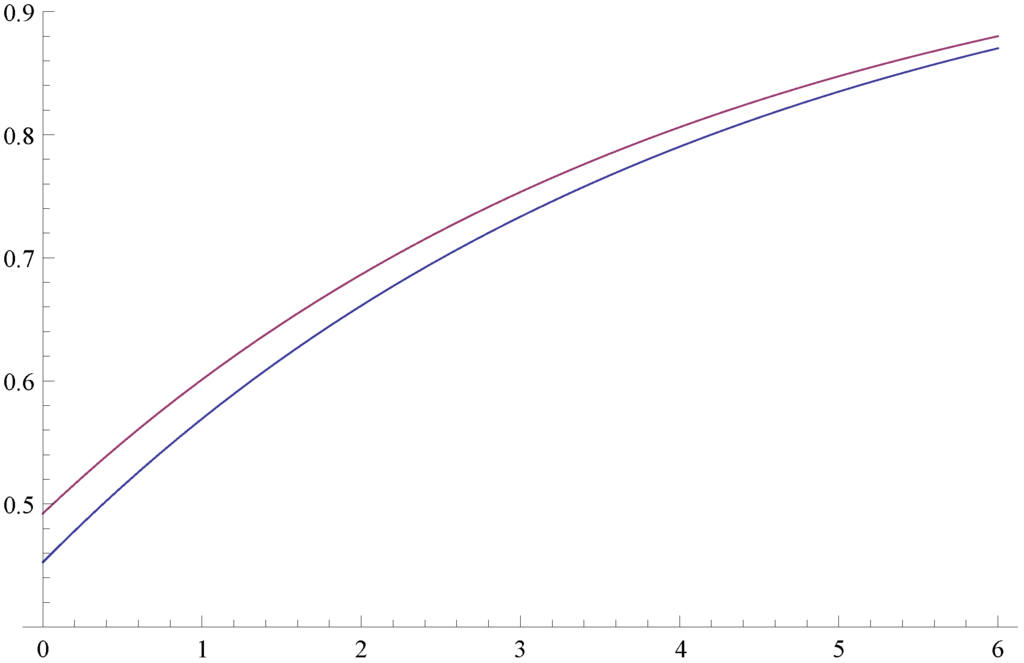
Figure 1. Survival probabilities, ${\varphi }_1\left(u\right)$ and ${\varphi }_2\left(u\right)$.

Figure 2 confirms the correctness of our results. It depicts ${\left(R\left(x\right)\mathbf{1}\right)}_1$ (i.e., the probability of reaching level x before being observed as being ruined when starting in State 1 with zero initial capital), and the dots represent Monte Carlo simulation estimates of the same quantity based on 10,000 runs, the horizontal line representing ${\varphi }_1\left(0\right)=0.45$. One sees that for large values of x, the numerical determination of $R\left(x\right)$ (as well as $\varphi \left(x\right)$) becomes a challenge, which underlines the importance of our limiting result, i.e., Theorem 4.2.

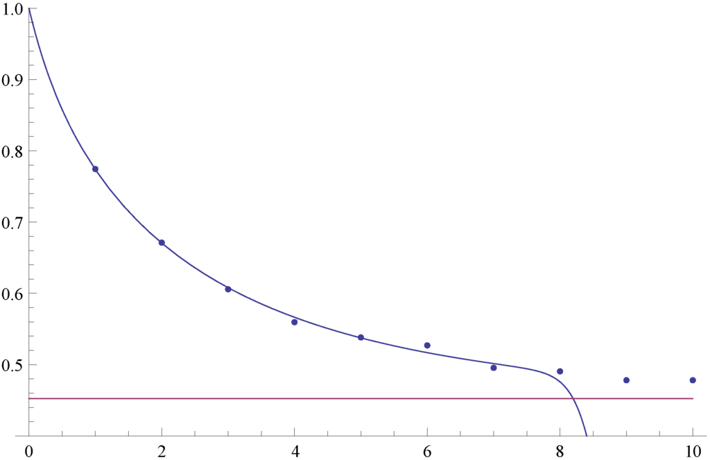
Figure 2. The probability of reaching level x before ruin for $J\left(0\right)=1,X\left(0\right)=0$.

References

- H. Albrecher, E.C.K. Cheung, and S. Thonhauser. “Randomized observation times for the compound Poisson risk model: Dividends.” Astin Bull. 41 (2011): 645–672. [Google Scholar]
- H. Albrecher, E.C.K. Cheung, and S. Thonhauser. “Randomized observation times for the compound Poisson risk model: The discounted penalty function.” Scand. Act. J. 6 (2013): 424–452. [Google Scholar] [CrossRef]
- H. Albrecher, and V. Lautscham. “From ruin to bankruptcy for compound Poisson surplus processes.” Astin Bull. 43 (2013): 213–243. [Google Scholar] [CrossRef]
- A. Dassios, and S. Wu. Parisian Ruin with Exponential Claims. Report; London, UK: Department of Statistics, London School of Economics and Political Science, 2008. [Google Scholar]
- R. Loeffen, I. Czarna, and Z. Palmowski. “Parisian ruin probability for spectrally negative Lévy processes.” Bernoulli 19 (2013): 599–609. [Google Scholar] [CrossRef]
- D. Landriault, J.F. Renaud, and X. Zhou. “Occupation times of spectrally negative Lévy processes with applications.” Stoch. Process. Appl. 121 (2011): 2629–2641. [Google Scholar] [CrossRef]
- S. Asmussen, and H. Albrecher. Ruin Probabilities, 2nd ed. Advanced Series on Statistical Science & Applied Probability, 14; Hackensack, NJ, USA: World Scientific Publishing Co. Pte. Ltd., 2010. [Google Scholar]
- H.U. Gerber, X.S. Lin, and H. Yang. “A note on the dividends-penalty identity and the optimal dividend barrier.” Astin Bull. 36 (2006): 489–503. [Google Scholar] [CrossRef]
- S. Asmussen, F. Avram, and M.R. Pistorius. “Russian and American put options under exponential phase-type Lévy models.” Stoch. Process. Appl. 109 (2004): 79–111. [Google Scholar] [CrossRef]
- J. Ivanovs. “One-Sided Markov Additive Processes and Related Exit Problems.” Ph.D. Dissertation, Uitgeverij BOXPress, Oisterwijk, The Netherlands, 2011. [Google Scholar]
- A.E. Kyprianou. Introductory Lectures on Fluctuations of Lévy Processes with Applications. Berlin, Germany: Springer-Verlag, 2006. [Google Scholar]
- L. Breuer. “First passage times for Markov additive processes with positive jumps of phase type.” J. Appl. Probab. 45 (2008): 779–799. [Google Scholar] [CrossRef] [Green Version]
- B. D’Auria, J. Ivanovs, O. Kella, and M. Mandjes. “First passage of a Markov additive process and generalized Jordan chains.” J. Appl. Probab. 47 (2010): 1048–1057. [Google Scholar] [CrossRef]
- J. Ivanovs, and Z. Palmowski. “Occupation densities in solving exit problems for Markov additive processes and their reflections.” Stoch. Process. Appl. 122 (2012): 3342–3360. [Google Scholar] [CrossRef]
- J. Ivanovs. “A note on killing with applications in risk theory.” Insur. Math. Econ. 52 (2013): 29–33. [Google Scholar] [CrossRef]
- D.E. Rutherford. “On the solution of the matrix equation AX + XB = C.” Ned. Akad. Wet. 35 (1932): 54–59. [Google Scholar]
- E. De Souza, and S.P. Bhattacharyya. “Controllability, observability and the solution of AX - XB = C.” Linear Algebra Appl. 39 (1981): 167–188. [Google Scholar] [CrossRef]
- Z. Jiang, and M.R. Pistorius. “On perpetual American put valuation and first-passage in a regime-switching model with jumps.” Financ. Stoch. 12 (2008): 331–355. [Google Scholar] [CrossRef]
- L. Breuer. “The resolvent and expected local times for Markov-modulated Brownian motion with phase-dependent termination rates.” J. Appl. Probab. 50 (2013): 430–438. [Google Scholar] [CrossRef]
- L. Breuer. “Threshold dividend strategies for a Markov-additive risk model.” Eur. Actuar. J. 1 (2011): 237–258. [Google Scholar] [CrossRef]
- L. Breuer. “Exit problems for reflected Markov-modulated Brownian motion.” J. Appl. Probab. 49 (2012): 697–709. [Google Scholar] [CrossRef]
- P. Lancaster. “Explicit solutions of linear matrix equations.” SIAM Rev. 12 (1970): 544–566. [Google Scholar] [CrossRef]
- J. Ivanovs. “Potential measures of one-sided Markov additive processes with reflecting and terminating barriers. arXiv.org e-Print archive.” 2013. Available online at http://arxiv.org/abs/1309.4987 (accessed on 11 October 2013).
© 2013 by the authors; licensee MDPI, Basel, Switzerland. This article is an open access article distributed under the terms and conditions of the Creative Commons Attribution license (http://creativecommons.org/licenses/by/3.0/).